Article

Risk Transfer among Housing Markets in Major Cities in China

1
Department of Finance, National University of Kaohsiung, No. 700, Kaohsiung University Rd., Nanzih District, Kaohsiung 811, Taiwan
2
Department of Finance, Chung Yuan Christian University, Taoyuan City 320, Taiwan
*
Author to whom correspondence should be addressed.
Sustainability 2018, 10(7), 2386; https://doi.org/10.3390/su10072386
Submission received: 11 June 2018 / Revised: 6 July 2018 / Accepted: 6 July 2018 / Published: 9 July 2018
(This article belongs to the Section Economic and Business Aspects of Sustainability)

Abstract

:
This study explored risk transfer among the housing markets of five major cities in China, comprising three first-tier cities (i.e., Beijing, Shanghai, and Shenzhen) and two second-tier cities (i.e., Tianjin and Chongqing). House price index data from January 2001 to June 2017 and a vector autoregressive–multivariate generalized autoregressive conditional heteroscedasticity model were employed to estimate correlations among these cities related to house price returns and volatility. In addition, volatility impulse-response functions were estimated to determine interactions among housing market risk in different cities. The results revealed that first-tier cities were more likely to transfer risk to second-tier cities, and that Beijing’s housing market exerted the greatest influence on risk in other cities’ housing markets. To consider the influence of the 2008 global financial crisis, data collected before and after the crisis were divided into two groups for subsequent investigation. The results revealed that these cities became more closely interrelated after the financial crisis, thereby escalating the risk of impulse influences. Finally, this study evaluated the influences of macroeconomic impulses on the housing markets of the three first-tier cities, indicating that real estate in these three cities can protect investors against inflation. The evidence presented in this paper can serve as a reference for the Chinese government regarding risk control.

1. Introduction

During the 19th Chinese Communist Party National Congress held in October 2017, a guideline for the development of the residential housing market in China was proposed, namely that “houses are for living, not for flipping”. After the congress, a new wave of housing policy reform was implemented. Before the end of October 2017, Poly Real Estate announced that its first real estate investment trust (REIT) had been approved by the Shanghai Stock Exchange. REITs are typical real estate securitization products that have a more-than-40-year history in the United States. By contrast, China has only quasi-REITs offered through private placement (REITs generally refer to publicly offered real estate funds); this shows the cautiousness of China’s supervisory authorities in relation to housing market risk control.
In the 2016–2017 policy campaign, the State Council, China Securities Regulatory Commission, and Ministry of Housing and Urban–Rural Development all vigorously promoted the release of REITs. Under the increasing risk of a housing market bubble, these government agencies claimed that the promotion of rental property-based REITs enables housing to return to its original function of providing a living space, thereby contributing to healthy and orderly development in the housing industry (please refer to an official notice by the Chinese government: House Building (2017), No. 153). This background illustrates an attempt of China’s supervisory authorities to control housing market risk and highlights the importance of risk in China’s housing market.
Reports by the International Monetary Fund have been issuing warnings against risk in China’s housing market since 2010; the reasons for these warnings have often focused on the excessively rapid speed of house price increases (Ahuja et al.) [1]. However, regardless of output, income, and house prices, China still lags behind Western countries by a considerable distance. In addition, after 2008, highly developed financial systems in advanced countries have been subject to skepticism, which may lead to capital concentration and substantial investment in the Chinese market. With respect to the catch-up effect, such investment would naturally cause markedly enhanced output and market growth. Viewing high growth as a source of risk may result in potential investors missing opportunities to invest in emerging markets. Thus, we believe that observing risk from the perspective of market volatility can provide more objective evaluation criteria.
Hence, this study employed the house price indices (HPIs) of five major cities in China from January 2001 to June 2017 to investigate the characteristics of housing market risk in various cities and the transmission of risk among various markets. The HPIs of three first-tier cities (i.e., Beijing, Shanghai, and Shenzhen) and two second-tier cities (i.e., Tianjin and Chongqing) were used to quantify interaction among housing market risk in different cities. According to economic development, the National Bureau of Statistics of the People’s Republic of China provide the city tier classification. The first- and second-tier cities are large and medium-sized cities in China. House prices in different tier cities may perform differently, for example, Shi et al. [2] found that after August 2015, housing prices in some second-tier cities, increased more quickly than first-tier cities.
This study adopted a model to simultaneously estimate co-movement of returns and risks among different markets and correlation between house price returns and volatility to produce a volatility impulse-response function. This enabled quantifying house price risk variation in first-tier cities with respect to the macroeconomic impulse. The remainder of this paper is organized as follows. Section 2 provides a review of related research on risk in China’s housing market. Section 3 describes an empirical model that illustrates how correlations between house price returns and volatility in different cities were simultaneously estimated in this study. Section 4 presents interactions between first- and second-tier cities regarding housing market risk and describes tests conducted to analyze the risk responses of major cities to macroeconomic impulse. Finally, Section 5 presents a conclusion that provides evidence for the control of market risks; the evidence could serve as a reference for competent authorities.

2. Literature Review

2.1. Housing Market Risk

Recently, the issue of housing market risk has been an important topic. For example, Banks et al. [3] developed a model on the effects of spatial housing price risk on housing choice. Chandler and Disney [4] explained why house prices are likely to be more volatile than prices in other markets, and considered the implications of variability in house prices for household behavior. Liu et al. [5] adopted data from 1981 to 2000 to examine the interrelationships between housing investment, non-housing investment, and economic growth in China throughout said period, and revealed that housing investment substantially influenced economic growth in the short term; hence, Liu et al. [5] noted that excessive dependence on real estate investment for economic growth can hamper the economic stability and safety of a country. Although housing investment can stimulate a country’s economy, it can also lead to negative outcomes; therefore, the government should implement strict control measures to limit housing investment growth. Deng et al. [6] maintained that irrational developments in the housing market and stock market between 2005 and 2010 were interrelated; their study further highlighted the importance of housing market risk in China. In summary, these studies asserted the importance of housing market risk and investment control for the Chinese government.
Many studies have approached the topic of China’s housing market performance from the question of whether a bubble exists in this market. Some studies have considered that house price performance in China is steered by fundamentals and that no bubble has been formed in this market. For example, Ren et al. [7] examined the annual return data on house prices in 35 Chinese cities throughout 1999–2009 and found that the return rates in China’s housing market did not satisfy the conditions of rational expectation bubbles. Shen [8] compared housing affordability in China and six developed countries; the results revealed that from 2002 to 2009, no bubble was detected in China’s real estate market. In addition, China’s market did not deteriorate from the perspective of housing affordability. Feng and Wu [9] adopted the equilibrium asset-pricing approach to review housing transaction data from 60 Chinese cities and determine whether a bubble existed in China’s real estate market. Regarding the average-price-to-rent ratio, the researchers’ results indicated that overall, no bubble existed in China’s real estate market.
In contrast to the aforementioned studies, numerous studies have detected bubbles in China’s housing market. For example, Hui and Yue [10] detected a bubble in Shanghai’s housing market in 2003, Hui and Gu [11] found bubbles in Guangzhou’s real estate market, the largest of which was that in 2007, which accounted for approximately 43% of the total market price. Hou [12] asserted that the house price cycle in Beijing can be divided into three periods, and bubbles began to emerge during 2005–2008; similarly, housing market bubbles were detected in Shanghai between 2003 and 2004. Gou and Li [13] revealed a relationship between an excess supply of money and house price bubbles in China. Yu [14] noted that although the housing markets in most Chinese cities have remained stable, those in some eastern metropolises such as Beijing, Shanghai, Shenzhen, Hangzhou, and Ningbo have developed bubbles since 2005. Dreger and Zhang [15] investigated 35 Chinese cities and found that house price bubbles were particularly prominent in southeastern coastal areas and special economic zones; by the end of 2009, bubbles in these areas accounted for approximately 25% of the total property value based on the fundamentals. Wang and Zhang [16] used China’s house price data from 2002 to 2008 to determine that house prices in several coastal cities were considerably higher than the level of the fundamentals. Shih, Li and Qin [17] examined 2000–2012 data from 28 Chinese provinces and observed that house price bubbles and housing affordability deterioration were more commonly observed in areas near Beijing and Shanghai. Liu et al. [18] investigated data from four major Chinese cities (i.e., Shanghai, Guangzhou, Shenzhen, and Beijing) and found evidence of bubbles between 1991 and 2011 in these cities.
Generally, the aforementioned studies show that housing market bubbles in Chinese cities are more prominent than the overall imbalance in China’s housing market. Whether house price overvaluation in individual cities generates risk in China’s national economy warrants investigation. Zhao et al. [19] stated that financial crises are typically derived from excess associations between an imperfect financial market and a country’s housing market; the researchers maintained that housing market bubbles exist in China and warned against a future crash. By contrast, Wu, Gyourko, and Deng [20] proposed that based on a limited number of samples, scholars should not discuss whether bubbles exist in China’s housing market. Wu, Gyourko and Deng [20] focused on the housing market risk and provided evidence supporting the existence of risk in China’s housing market and indicated problems that must be resolved such as high house price growth rates in some cities, land price decreases, and between-city variations in the supply-demand balance of the housing market. The present study also adopted the perspective of housing market risk to evaluate the origins and transfer of risk among China’s major cities.

2.2. The Estimation of Housing Market Risk

This study investigated risk transfer among the housing markets of five major cities in China. Two models are often adopted to analyze correlations among markets; the vector autoregressive (VAR) model is used to evaluate the relationships of return on assets among markets, whereas the multivariate generalized autoregressive conditional heteroscedasticity (MGARCH) model is adopted to estimate the correlation between return on assets and volatility (risk). Chowdhury and Maclennan [21] used a Markov switching VAR model to test the regional housing markets in the UK; Lee and Reed [22] used a GARCH model to obtain the volatility decomposition of Australian housing prices. Karolyi [23] employed the VAR and MGARCH models to separately estimate stock returns and risk transfer across various countries; however, because the VAR and MGARCH models were estimated separately, the results in Karolyi [23] did not determine whether the correlation was derived from returns or risk.
Several recent studies have adopted a VAR–MGARCH model for estimation. Such a model enables more comprehensive quantification of between-market correlation because both returns and risks are endogenous variables that can be explained by the same functions in a model. The VAR–MGARCH model supports the incorporation of multiple variables and determines whether between-variable influences are derived from returns or volatility. Such models have been extensively used to evaluate markets with different assets. For example, Bekiros [24] explored the relationship between exchange rate volatility and fundamentals; Sogiakas and Karathanassis [25] evaluated spot and derivatives markets; Jiang et al. [26] estimated the U.S. crude oil, corn, and plastics markets; and Andreasson et al. [27] assessed interactions between commodity futures returns and five driving factors. The VAR model has another strength; it can quantify the influences that the impulses of factors have on market returns.
In other words, the VAR model supports impulse-response analysis. Adding heterogeneous variances of volatility in the VAR model increases the soundness of impulse-response analysis. For example, Elder [28] derived an impulse-response function for a vector autoregression with multivariate GARCH errors; Conrad and Karanasos [29] explicated the impulse-response function of volatility; Hafner and Herwartz [30] used exchange rate data to estimate the volatility impulse-response function (VIRF) under an MGARCH model; and Le Pen and Sévi [31] expanded the model developed by Hafner and Herwartz [30] by using daily data from March 2001 to June 2005 to formulate a VAR–MGARCH model and obtain a VIRF to evaluate and find evidence of return and volatility spillovers among the German, Dutch, and British forward electricity markets.
Tian and Gallagher [32] detected conspicuous volatility in China’s housing market from 2005 to 2013 and found that short-term overseas capital flows ameliorated house price growth in China; however, hot money enhanced the effect of capital flows on house prices. Weng and Gong [33] used the HPIs of ten major Chinese cities from January 2005 to December 2014 to analyze volatility spillover effects and identify the determinants of price co-movement across China’s regional housing markets; the results revealed that house prices in cities are primarily influenced by population, income, mortgage rates, policy factors, and macroeconomic conditions at the national level. The results of Weng and Gong [33] also confirmed that correlations among China’s regional housing markets exist. If cities are subject to the influence of certain impulses and exhibit risk spillover, risk in China’s overall housing market can cause detrimental damage to macroeconomics, regardless of whether house prices are high. Therefore, the present study investigated risk transfer among housing market risks in five major cities in China to quantify these risks and compare their sources.
Thus, the present study adopted a VAR–MGARCH model to evaluate risk transfer among housing markets and used a VIRF to quantify the effects of macroeconomic factors on house price risk. In addition, this study used the four variables to detect the effects of macroeconomic factors, these variables are money supply, interest rate, consumer price index, and balance of fiduciary loan. Numerous studies have verified that monetary policies can trigger housing market risks. For example, Shiller [34] found that the variations of the real federal fund rates can explain the housing boom. McDonald and Stokes [35] provided the evidence showing that monetary policy produced the housing price bubble. Previous studies on housing bubbles have indicated the importance of monetary policies (Liang and Cao [36], Gou and Li [13], Tsai [37]). Liang and Cao [36] observed a significant influence of bank lending on China’s real estate prices, and Gou and Li [13] have noted that currency liquidity can affect house prices in China’s housing market. Tsai [37] found the evidence showing the correlations between monetary liquidity and house price bubbles in the US housing market. Following these studies, we employed the four variables related to monetary policies to estimate the VIRF.

3. Empirical Model

3.1. Model for the Estimation of Housing Market Risk

To illustrate house price risk transfer among Chinese cities, the present study adopted the VAR–MGARCH model to formulate a VIRF for analyzing factors influential to house price risk. Five cities were examined in our study. The cities are three first-tier cities (i.e., Beijing, Shanghai, and Shenzhen) and two second-tier cities (i.e., Tianjin and Chongqing). The HPI data of these cities were provided by the SouFun Company (Beijing, China) and the remaining items were retrieved from the China Real Estate Index System. To further clarify market correlations, these cities were paired to evaluate their relationships. The proposed model is presented as follows; let the vector of house price return be r x = [ r x 1   r x 2 ]. The equations for the conditional average of the return are
[ r x 1 , t r x 2 , t ] = [ i = 1 n φ 11 , i r x 1 , t i i = 1 n φ 21 , i r x 1 , t i ] + [ i = 1 n φ 12 , i r x 2 , t i i = 1 n φ 21 , i r x 2 , t i ] + [ ε x 1 , t ε x 2 , t ]
ε t | Ω t 1 = [ ε x 1 , t ε x 2 , t ] | Ω t 1 ~ N ( 0 ,   H t )
and that for the conditional variance of the return is
H t = [ c 11 0 c 21 c 22 ] + [ a 11 a 12 a 21 a 22 ] e t 1 e t 1 [ a 11 a 12 a 21 a 22 ] + [ b 11 b 12 b 21 b 22 ] H t 1 [ b 11 b 12 b 21 b 22 ]
where r x represents the city’s house price returns. a i i , b i i , c i i are volatility-related coefficients.

3.2. The Estimation for VIRF

After estimating correlations among the five cities, this study analyzed the sources of risk in the three first-tier cities. We employed the four variables related to monetary policies to estimate the VIRF. M2 statistics, the 1-year loan interest rate, the consumer price index, and the total amount of fiduciary loans were adopted to represent money supply, short-term interest rate, price index, and balance of fiduciary loans, respectively. We also adopted the VAR–MGARCH model to estimate the relationship between the house price return of the investigated city and the change rate of macroeconomic variables. The VAR–MGARCH model is as follows.
[ r x , t r M a c , t ] = [ i = 1 n φ 11 , i r x , t i i = 1 n φ 21 , i r x , t i ] + [ i = 1 n φ 12 , i r M a c , t i i = 1 n φ 21 , i r M a c , t i ] + [ ε x , t ε M a c ,   t ]
ε t | Ω t 1 = [ ε x , t ε M a c ,   t ] | Ω t 1 ~ N ( 0 ,   H t )
and that for the conditional variance of the return is
H t = [ c 11 0 c 21 c 22 ] + [ a 11 a 12 a 21 a 22 ] e t 1 e t 1 [ a 11 a 12 a 21 a 22 ] + [ b 11 b 12 b 21 b 22 ] H t 1 [ b 11 b 12 b 21 b 22 ]
where r x represents the house price return of the investigated city. r M a c represents the growth rate of macroeconomic variables, including money supply, short-term rate, CPI and loan balance. a i i , b i i , c i i are volatility-related coefficients. Then we used the results of the estimation to formulate a VIRF for analyzing factors influential to house price risk.

4. Results

Table 1 lists the basic statistics of the data used in this study, which consisted of the HPIs of the five cities and four monetary variables (i.e., money supply, short-term interest rate, price index, and balance of fiduciary loans). This study adopted monthly frequency data from January 2001 to June 2017. Table 1 lists data characteristics such as HPI return rates and macroeconomic variable growth rates. PP is the PP unit root test, which is adopted for testing the null hypothesis of a unit root in the series. The lag length of the unit root models is selected by using the Schwarz information criterion. According to the unit root test results (Table 1), the house price return rates of the five cities and growth rates of the four macroeconomic variables were all stationary data that could be used to estimate the VAR model. J-B is The Jarque-Bera statistic which has a chi-square distribution under the null hypothesis of normal distribution. The Jarque-Bera test statistic showed that all data strongly rejected the assumption of normal distribution. L-B Q(n) are Ljung-Box statistics for testing whether there is serial correlation in series, n denotes lag term. The Ljung-Box test statistic indicated that all variables exhibited self-correlation.
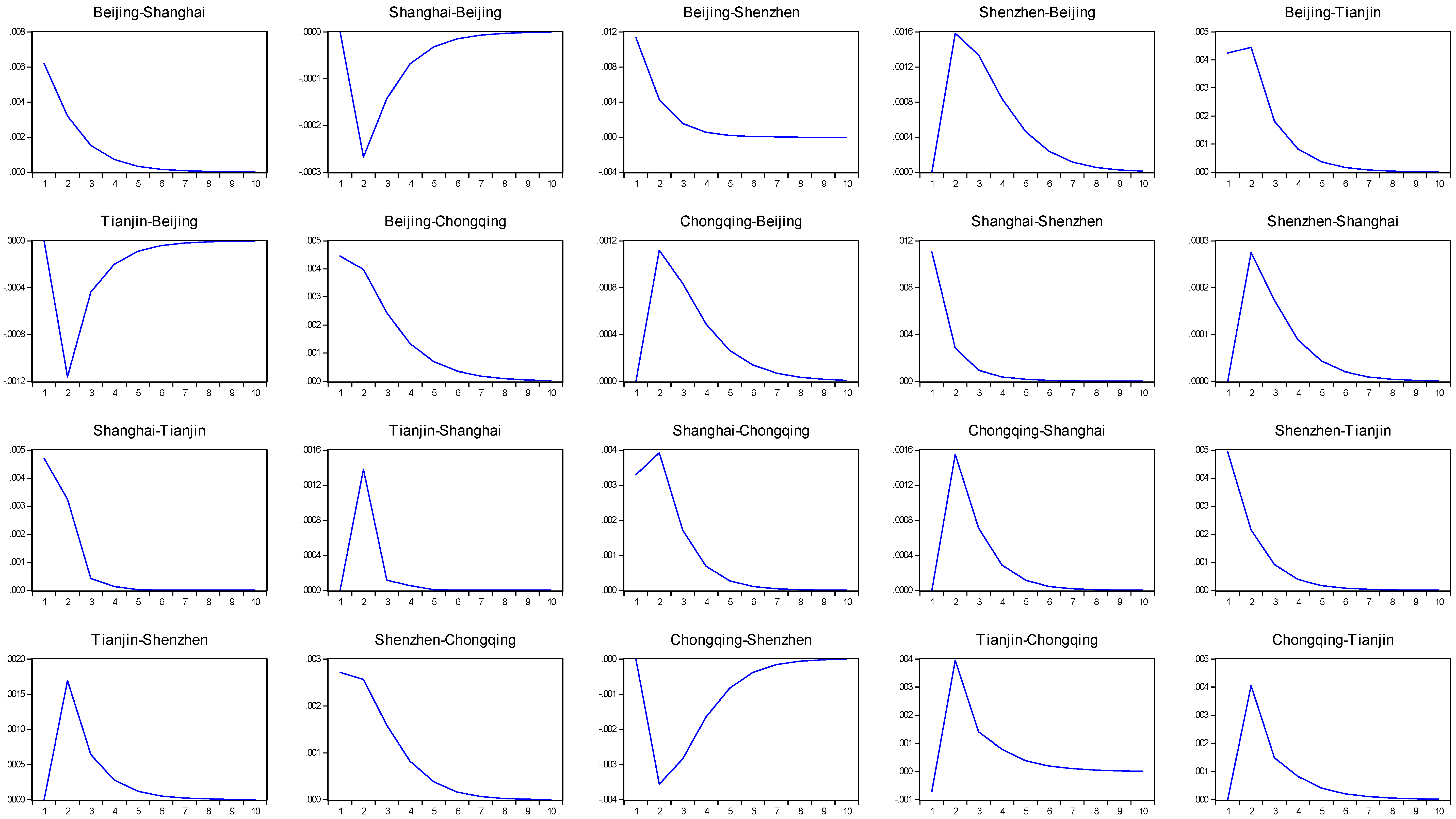
A conventional VAR model was employed to evaluate the interrelationships among the five cities with respect to house price returns. The results showed that no between-city correlations in house price returns were significant (Table 2). Only the returns in Beijing positively influenced those in Shanghai and Tianjin; those in Tianjin and Chongqing exhibited positive interaction; and those in Chongqing negatively influenced those in Shenzhen. To further clarify the extents of these influences, Figure 1 illustrates the impulse-response function estimated using the VAR model (Table 2). The correlations within city pairs are listed, with the first city in each diagram indicating the impulse source and the second city indicating the city responding to the impulse. Figure 1 shows that the greatest impulse that every city sustained was generated by itself and the impulses in Beijing’s housing market exerted the most conspicuous influence on other cities. Many of the city pairs shown in Figure 1 did not exhibit significant relationships, such as the influence of Shanghai’s impulses on Beijing. Moreover, the influence of cities other than Beijing on Shanghai approximated 0; this observation might be attributable to how cities other than Beijing likely exhibited housing market variations consistent with those in Beijing, and thus their influences could not be discerned from a model of joint estimation.
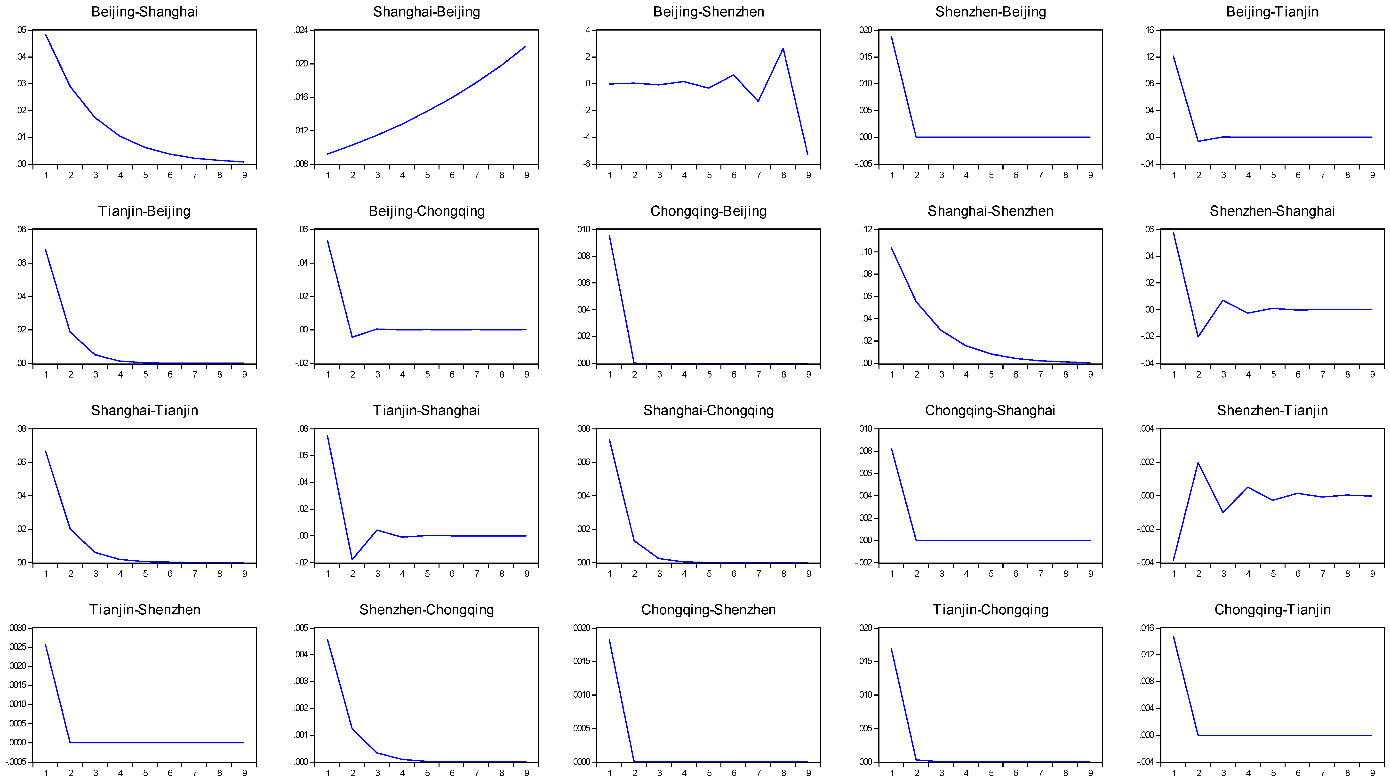
In Table 3, VAR models of city pairs are presented to show interaction between cities. Because we used house price return data of five cities, ten VAR models are displayed. In terms of correlation between return rates, the results in Table 3 are much higher than those in Table 2. Only two city combinations had no significant correlation between returns, namely Beijing & Shenzhen and Shanghai & Shenzhen. We illustrated the impulse-response function estimated based on Table 3 in Figure 2 and found that the impulse influences in Figure 2 were greater than those in Figure 1. However, Table 3 does not cover correlations of volatility. Table 4 presents the estimation results obtained using the VAR–MGARCH model (Equations (1)–(3)) to provide a more comprehensive analysis. Except for Shanghai & Shenzhen and Shenzhen & Chongqing, lead-lag relationships existed in all city pairs. In other words, a return spread effect existed. Specifically, house price returns in Beijing influenced those in Shanghai and Shenzhen and were influenced by those in Tianjin and Chongqing. House price returns in Shanghai and Shenzhen influenced those in Tianjin, those in Tianjin influenced those in Chongqing, and those in Chongqing reversely influenced those in Shanghai. These relationships suggested that among the first-tier cities, Beijing was the source of influence for Shanghai and Shenzhen. Shanghai and Shenzhen mainly influenced the second-tier city Tianjin, which further influence Chongqing, and through the latter, the influence was transferred back to Beijing and Shanghai.
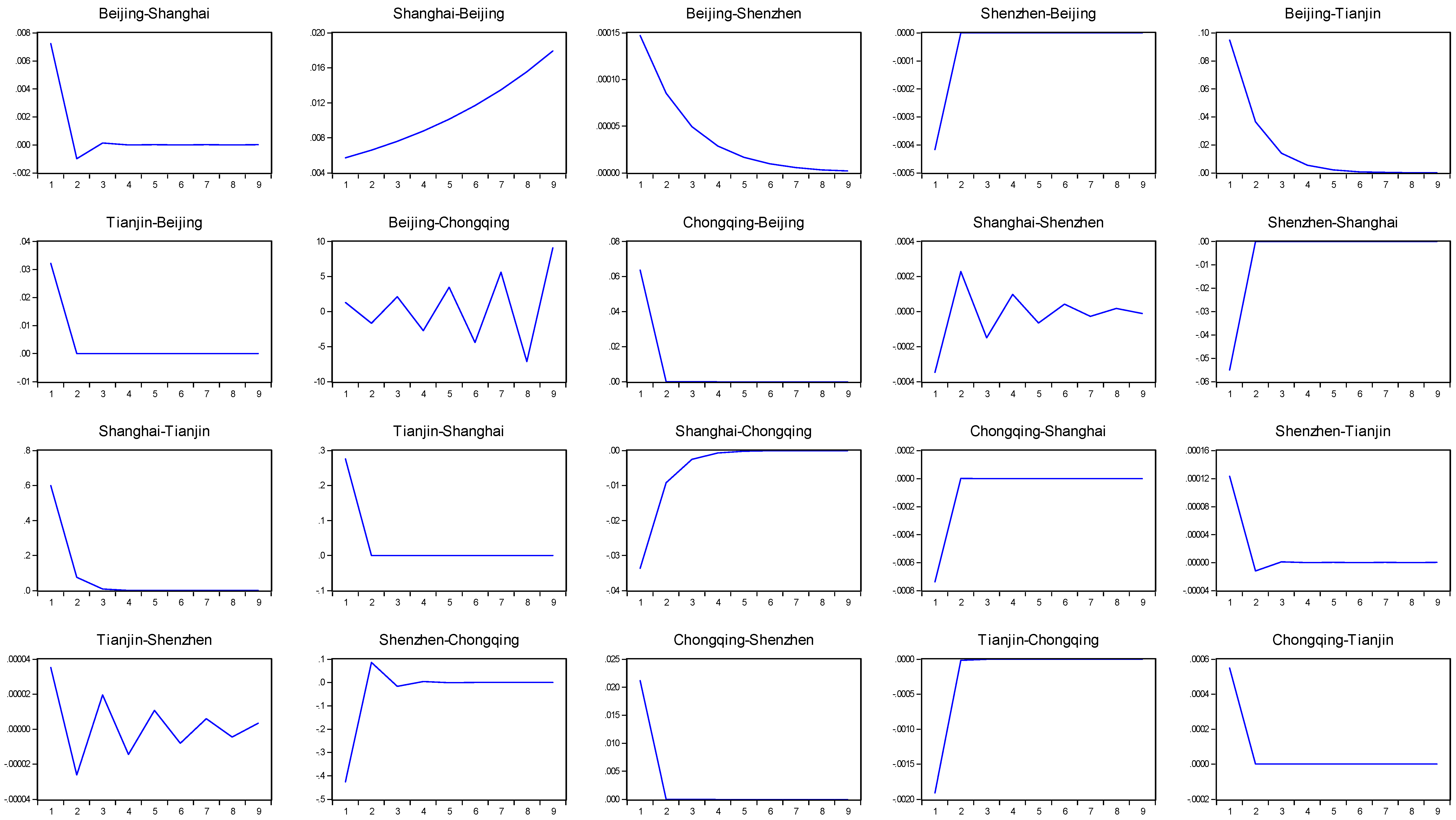
The aforementioned notable lead-lag relationships indicated that the analyzed cities may also transfer risk among themselves. From the estimation results of the volatility matrix presented in Table 4, regardless of whether a lead-lag relationship existed between paired cities, all pairs achieved significant correlation in terms of volatility. The estimation results revealed that several of the correlation functions had all their volatility-related coefficients (i.e., a 12 , a 21 , b 12 , b 21 , a 12 , or c 12 ) achieving significance, and some of the functions had at least one of the coefficients achieving significance. The VIRF obtained based on Table 3 is illustrated in Figure 3. The figure shows that the influences of volatility between paired cities were all positive. In other words, impulses in the housing market of one city result in increases in the housing market of another city. However, these influences can be divided into two types. The first type causes volatility that increases over time, whereas the second type causes volatility that decreases over time. In other words, Type 1 influences are those that scale up a crisis when transferring risk from one market to another, whereas Type 2 influences are those that temporarily increase risk during such transfers, and the influences are undermined over time. The most prominent example of a Type 1 influence was the transference of impulses from Shanghai’s housing market to Beijing’s housing market.
The evaluation results in Table 2, Table 3 and Table 4 all indicate that Beijing exerted the greatest influence on the other cities. When risks were derived in Shanghai, they were transferred to the second-tier cities through Beijing and eventually transferred back to Beijing and Shanghai. Evidently, such market instability leads to systematic crises. Previous studies have shown that in 2003, a bubble was first developed in Shanghai’s housing market (Hui and Yue [10], Hou [12]). Shortly after, greater bubbles were observed in Beijing’s housing market (Hou [12]) and even in some second-tier coastal cities (Shih, Li, and Qin [17]). Thus, although instabilities in Beijing’s housing market have the greatest influence on other cities, a systematic crisis is more likely to emerge if such instabilities are derived from Shanghai’s influence on Beijing.
The Type 2 influences observed in this study involved a gradual reduction in responses to volatility and could be further categorized into fast-decreasing and slow-decreasing influences. Fast-decreasing influences included Chongqing’s influence on Beijing and Shenzhen, as well as Shenzhen’s influence on Beijing; whereas slow-decreasing influences included Shanghai’s influence on Shenzhen and Shenzhen’s influence on Chongqing. The more rapidly responses to volatility decrease, the easier it becomes for the influenced housing market to undermine increased risks and the less likely is a systematic crisis to be formed. Figure 3 shows that most of the influences exerted by second-tier cities on first-tier cities were slow decreasing; this finding entailed stability in first-tier cities.
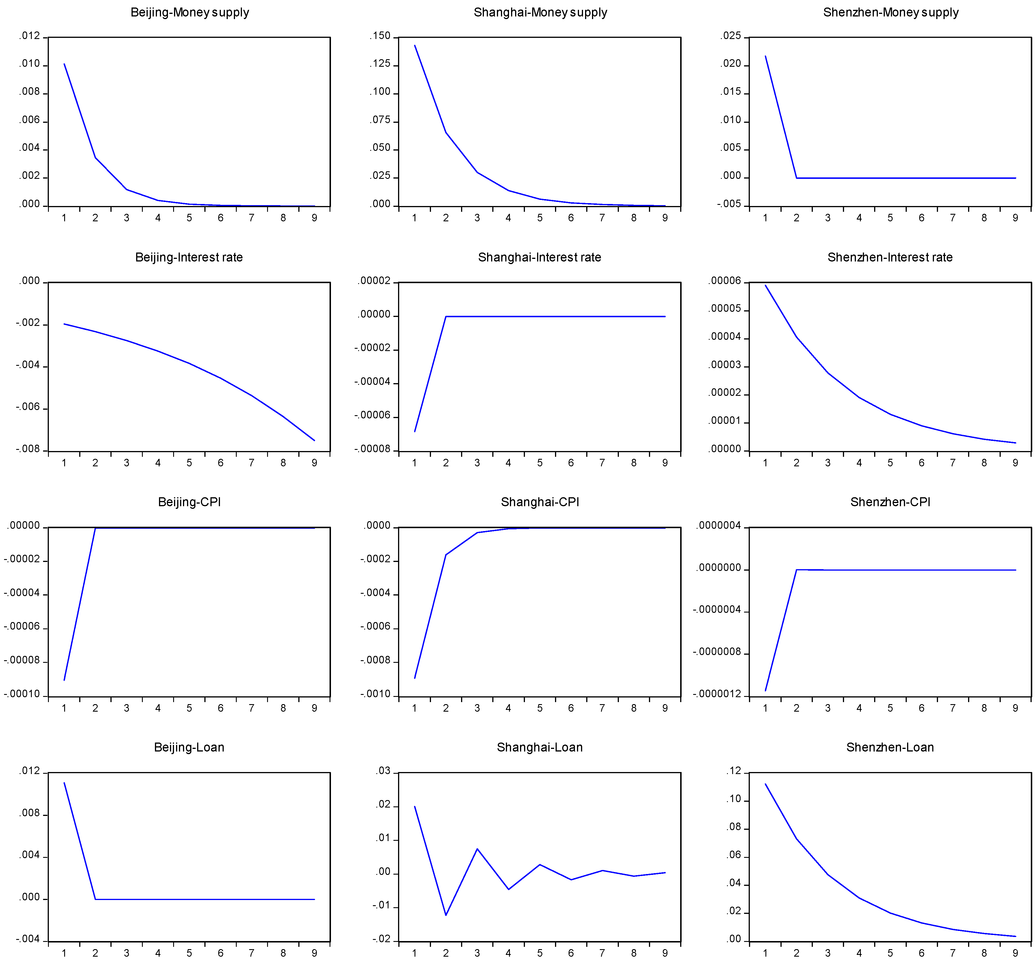
In the following discussion, we adopted September 2008 as the baseline to divide the sample data into those before and after the 2008 financial crisis. Estimations were subsequently performed using the VAR–MGARCH model, and VIRFs were calculated. The VIRFs before and after the financial crisis are illustrated in Figure 4 and Figure 5, respectively. Comparing Figure 4 and Figure 5 revealed that these cities became more closely interrelated after the financial crisis, evidenced by volatility increases derived from impulses growing in terms of extent and duration. In addition, although impulses from Shanghai remained those most likely to expand to systematic risks, the transfer channel shifted. Before the crisis, most systematic risks were generated by risks transferred from Shanghai to Beijing; whereas after the crisis, systematic risks were transferred first from Shanghai to Shenzhen and subsequently from Shenzhen to Tianjin. This finding could serve as a reference for competent authorities to discern the potential for future systematic crises in China’s housing market.
Regarding how risk transfer can be prevented, four monetary macroeconomic variables were adopted in this study to identify the sources of risks in the three first-tier cities. The VAR–MGARCH models (Equations (4)–(6)) for Beijing, Shanghai, and Shenzhen based on the four variables are listed in Table 5, Table 6 and Table 7, respectively. Figure 6 illustrates the impulse influences of the four variables on the volatility of house price returns in these three cities. The estimation results showed that on average, only price index increases in the previous period resulted in increases in Beijing’s house price returns (Table 5). Regarding the influence on risk, raising interest rates was the most effective measure for controlling Beijing’s housing market risks because it enabled continuous risk reduction (Figure 6). As indicated by Table 6 and Figure 6, impulses from money supply were most likely to substantially increase Shanghai’s housing market risks. Furthermore, impulses from fiduciary loans caused instability in Shenzhen’s housing market, leading to considerable growth in volatility and a slower influence reduction rate (Table 7 and Figure 6). Finally, analyzing the results in Figure 6 revealed that impulses derived from price index growth immediately lowered the risks in the housing markets of the three first-tier cities, indicating that these housing markets can protect investors against inflation. Overall, the results of Table 5 and Table 6 indicated that a marked increase in money supply can lead to excess impulse influence and risk escalation in Shanghai’s housing market. When such risks are transferred to the housing market in Beijing or Shenzhen, excessively high systematic risks tend to occur in China’s housing market.

5. Conclusions

In this study, HPI data of three first-tier cities (i.e., Beijing, Shanghai, and Shenzhen) and two second-tier cities (i.e., Tianjin and Chongqing) in China from January 2001 to June 2017 and VAR–MGARCH models were employed to calculate correlations in house price returns and volatility among these cities. In addition, VIRFs were obtained to analyze risk transfer among the housing markets of these cities. Furthermore, correlations in four monetary variables (i.e., money supply, short-term interest rate, price index, and balance of fiduciary loans) among the three first-tier cities were analyzed to determine the sources of risk in specific cities. The results revealed that between-city risk transfers originated in Beijing and were transferred to the other two first-tier cities. Shanghai and Shenzhen primarily influenced the second-tier city of Tianjin, which further transferred risks to Chongqing and subsequently back to Beijing or Shanghai. The evaluation results of the influences of volatility impulses revealed that although instabilities in Beijing’s housing market had the greatest influence on the housing markets of the other cities, a systematic crisis is more likely to emerge if such instabilities are derived from Shanghai’s influence on Beijing. Moreover, systematic risks in China’s housing market can escalate through the aforementioned transfer channel.
To consider the influence of the 2008 global financial crisis, data collected before and after the crisis were divided into two groups for subsequent investigation. The results revealed that the five analyzed cities became more closely interrelated after the financial crisis, evidenced by volatility increases derived from impulses growing in terms of extent and duration. Moreover, the risk transfer from Shanghai to Shenzhen and further to Tianjin warrants particular attention.
Finally, this study evaluated the influences of macroeconomic impulses on the housing markets of three first-tier cities. The results revealed the following findings. (1) The primary risks in Shanghai’s housing market are generated by monetary impulses. (2) Volatility in Beijing’s housing market can be effectively controlled by implementing policies related to interest rates; specifically, interest rate increases can lower risk in Beijing’s housing market. (3) The main risks in Shenzhen’s housing market are generated by fiduciary loan impulses, which cause instability in the market, substantially increase volatility, and exert influences that decrease in severity at lower rates. We summarized the evaluation results of between-city risk transfer and risk sources in first-tier cities and found that considerable increases in money supply markedly increased risk in Shanghai’s housing market. When risk is transferred to the housing markets of Beijing or Shenzhen, excessive systematic risk tends to occur in China’s housing market. This finding supports a previous finding in the literature, namely that excess monetary liquidity can cause bubbles in China’s housing market.
The estimation results of this study provided objective evidence of two topics of risk. First, the results elucidated interactions between housing market risk in first- and second-tier cities. Second, the results could be used to test the responses of major cities to macroeconomic impulse. Exploring the first of these two topics facilitated determining whether substantial growth in China’s housing market will lead to a systematic crisis similar to that before the subprime mortgage crisis in the United States. Furthermore, we compared data from the United States before and after the 2008 financial crisis to determine whether the risk of such a systematic crisis is growing. The second topic focused on how to regulate the sources of risk affecting major Chinese cities’ housing markets. The results indicated that the major risks in Shanghai’s housing market were generated by monetary factors, whereas those in Shenzhen’s housing market were generated by increases in fiduciary loans. Moreover, interest rate policy is the most effective factor for suppressing the volatility in Beijing’s housing market.
Instead of approaching this topic from the perspective of bubbles, this study focused on objective quantification and analyzing risk in China’s housing market, delineating risk transfer among housing markets in different cities, and exploring effective measures to control the main risk sources of the three first-tier cities. The perspectives and evidence presented in this paper can serve as a reference for the Chinese government regarding risk control; moreover, they can serve as a more objective basis for traders interested in China’s housing market in terms of evaluating investment opportunities in this emerging market characterized by high growth.

Author Contributions

S.-H.C. provided and analyzed the data. I.-C.T. contributed formal analysis, investigation, and writing.

Funding

Funding from the Ministry of Science and Technology of Taiwan under Project No. MOST-104-2410-H-390-028-MY3 has enabled the continuation of this research and the dissemination of these results.

Conflicts of Interest

The authors declare no conflict of interest.

References

  1. Ahuja, A.; Cheung, L.; Han, G.; Porter, N.; Zhang, W. Are House Prices Rising too Fast in China? IMF Working Paper No. 10/274; International Monetary Fund: Washington, DC, USA, 2011. [Google Scholar]
  2. Shi, G.; Liu, X.; Zhang, X. Time-varying causality between stock and housing markets in China. Financ. Res. Lett. 2017, 22, 227–232. [Google Scholar] [CrossRef]
  3. Banks, J.; Blundell, R.; Oldfield, Z.; Smith, J.P. Housing Price Volatility and Housing Ownership over the Lifecycle; Discussion Papers in Economics 04-09; University College London: London, UK, 2004. [Google Scholar]
  4. Chandler, D.; Disney, R. The housing market in the United Kingdom: Effects of house price volatility on households. Fisc. Stud. 2014, 35, 371–394. [Google Scholar] [CrossRef]
  5. Liu, H.; Park, Y.W.; Zheng, S. The interaction between housing investment and economic growth in China. Int. Real Estate Rev. 2002, 5, 40–60. [Google Scholar]
  6. Deng, Y.; Girardin, E.; Joyeux, R.; Shi, S. Did bubbles migrate from the stock to the housing market in China between 2005 and 2010? Pac. Econ. Rev. 2017, 22, 276–292. [Google Scholar] [CrossRef]
  7. Ren, Y.; Xiong, C.; Yuan, Y. House price bubbles in China. China Econ. Rev. 2012, 23, 786–800. [Google Scholar] [CrossRef]
  8. Shen, L. Are house prices too high in China? China Econ. Rev. 2012, 23, 1206–1210. [Google Scholar] [CrossRef]
  9. Feng, Q.; Wu, G.L. Bubble or riddle? An asset-pricing approach evaluation on China’s housing market. Econ. Model. 2015, 46, 376–383. [Google Scholar] [CrossRef]
  10. Hui, E.C.M.; Yue, S. Housing price bubbles in Hong Kong, Beijing and Shanghai: A comparative study. J. Real Estate Financ. Econ. 2006, 33, 299–327. [Google Scholar] [CrossRef]
  11. Hui, E.C.M.; Gu, Q. Study of Guangzhou house price bubble based on state-space model. Int. J. Strateg. Prop. Manag. 2009, 13, 287–298. [Google Scholar]
  12. Hou, Y. Housing price bubbles in Beijing and Shanghai? A multi-indicator analysis. Int. J. Hous. Mark. Anal. 2010, 3, 17–37. [Google Scholar] [CrossRef]
  13. Guo, S.; Li, C. Excess liquidity, housing price booms and policy challenges in China. China World Econ. 2011, 19, 76–91. [Google Scholar] [CrossRef]
  14. Yu, H. Size and characteristic of housing bubbles in China’s major cities: 1999–2010. China World Econ. 2011, 19, 56–75. [Google Scholar] [CrossRef]
  15. Dreger, C.; Zhang, Y. Is there a bubble in the Chinese housing market? Urban Policy Res. 2013, 31, 27–39. [Google Scholar] [CrossRef]
  16. Wang, Z.; Zhang, Q. Fundamental factors in the housing markets of China. J. Hous. Econ. 2014, 25, 53–61. [Google Scholar] [CrossRef]
  17. Shih, Y.-N.; Li, H.-C.; Qin, B. Housing price bubbles and inter-provincial spillover: Evidence from China. Habitat Int. 2014, 43, 142–151. [Google Scholar] [CrossRef]
  18. Liu, R.; Hui, E.C.M.; Lv, J.; Chen, Y. What drives housing markets: Fundamentals or bubbles? J. Real Estate Financ. Econ. 2017, 55, 395–415. [Google Scholar] [CrossRef]
  19. Zhao, S.X.B.; Zhan, H.; Jiang, Y.; Pan, W. How big is China’s real estate bubble and why hasn’t it burst yet? Land Use Policy 2017, 64, 153–162. [Google Scholar] [CrossRef]
  20. Wu, J.; Gyourko, J.; Deng, Y. Evaluating the risk of Chinese housing markets: What we know and what we need to know. China Econ. Rev. 2016, 39, 91–114. [Google Scholar] [CrossRef] [Green Version]
  21. Chowdhury, R.A.; Maclennan, D. Regional house price cycles in the UK, 1978–2012: A Markov switching VAR. J. Eur. Real Estate Res. 2014, 7, 345–366. [Google Scholar] [CrossRef]
  22. Lee, C.L.; Reed, R. Volatility decomposition of Australian housing prices. J. Hous. Res. 2013, 23, 21–43. [Google Scholar]
  23. Karolyi, G.A. A Multivariate GARCH Model of international transmissions of stock returns and volatility: The case of the United States and Canada. J. Bus. Econ. Stat. 1995, 13, 11–25. [Google Scholar]
  24. Bekiros, S.D. Exchange rates and fundamentals: Co-movement, long-run relationships and short-run dynamics. J. Bank. Financ. 2014, 39, 117–134. [Google Scholar] [CrossRef]
  25. Sogiakas, V.; Karathanassis, G. Informational efficiency and spurious spillover effects between spot and derivatives markets. Glob. Financ. J. 2015, 27, 46–72. [Google Scholar] [CrossRef] [Green Version]
  26. Jiang, J.; Thomas, T.L.; Tozer, P.R. Policy induced price volatility transmission: Linking the U.S. crude oil, corn and plastics markets. Energy Econ. 2015, 52, 217–227. [Google Scholar] [CrossRef]
  27. Andreasson, P.; Bekiros, S.; Nguyen, D.K.; Uddin, G.S. Impact of speculation and economic uncertainty on commodity markets. Int. Rev. Financ. Anal. 2016, 43, 115–127. [Google Scholar] [CrossRef]
  28. Elder, J. An impulse-response function for a vector autoregression with multivariate GARCH-in-mean. Econ. Lett. 2003, 79, 21–26. [Google Scholar] [CrossRef] [Green Version]
  29. Conrad, C.; Karanasos, M. The impulse response function of the long memory GARCH process. Econ. Lett. 2006, 90, 34–41. [Google Scholar] [CrossRef]
  30. Hafner, C.M.; Herwartz, H. Volatility impulse responses for multivariate GARCH models: An exchange rate illustration. J. Int. Money Financ. 2006, 25, 719–740. [Google Scholar] [CrossRef]
  31. Le Pen, Y.; Sévi, B. Volatility transmission and volatility impulse response functions in European electricity forward markets. Energy Econ. 2010, 32, 758–770. [Google Scholar] [CrossRef]
  32. Tian, Y.; Gallagher, K.P. Housing Price Volatility and the Capital Account in China; GEGI Working Paper; Global Economic Governance Initiative: Boston, MA, USA, 2015. [Google Scholar]
  33. Weng, Y.; Gong, P. On price co-movement and volatility spillover effects in China’s housing markets. Int. J. Strateg. Prop. Manag. 2017, 21, 240–255. [Google Scholar] [CrossRef]
  34. Shiller, R.J. Understanding Recent Trends in House Prices and Homeownership. In Housing, Housing Finance and Monetary Policy; Jackson Hole Conference Series; Federal Reserve Bank of Kansas: Kansas City, MO, USA, 2008; pp. 85–123. [Google Scholar]
  35. McDonald, J.F.; Stokes, H.H. Monetary policy and the housing bubble. J. Real Estate Financ. Econ. 2013, 46, 437–451. [Google Scholar] [CrossRef]
  36. Liang, Q.; Cao, H. Property prices and bank lending in China. J. Asian Econ. 2007, 18, 63–75. [Google Scholar] [CrossRef]
  37. Tsai, I.-C. Monetary liquidity and the bubbles in the U.S. housing market. Int. J. Strateg. Prop. Manag. 2015, 19, 1–12. [Google Scholar] [CrossRef]
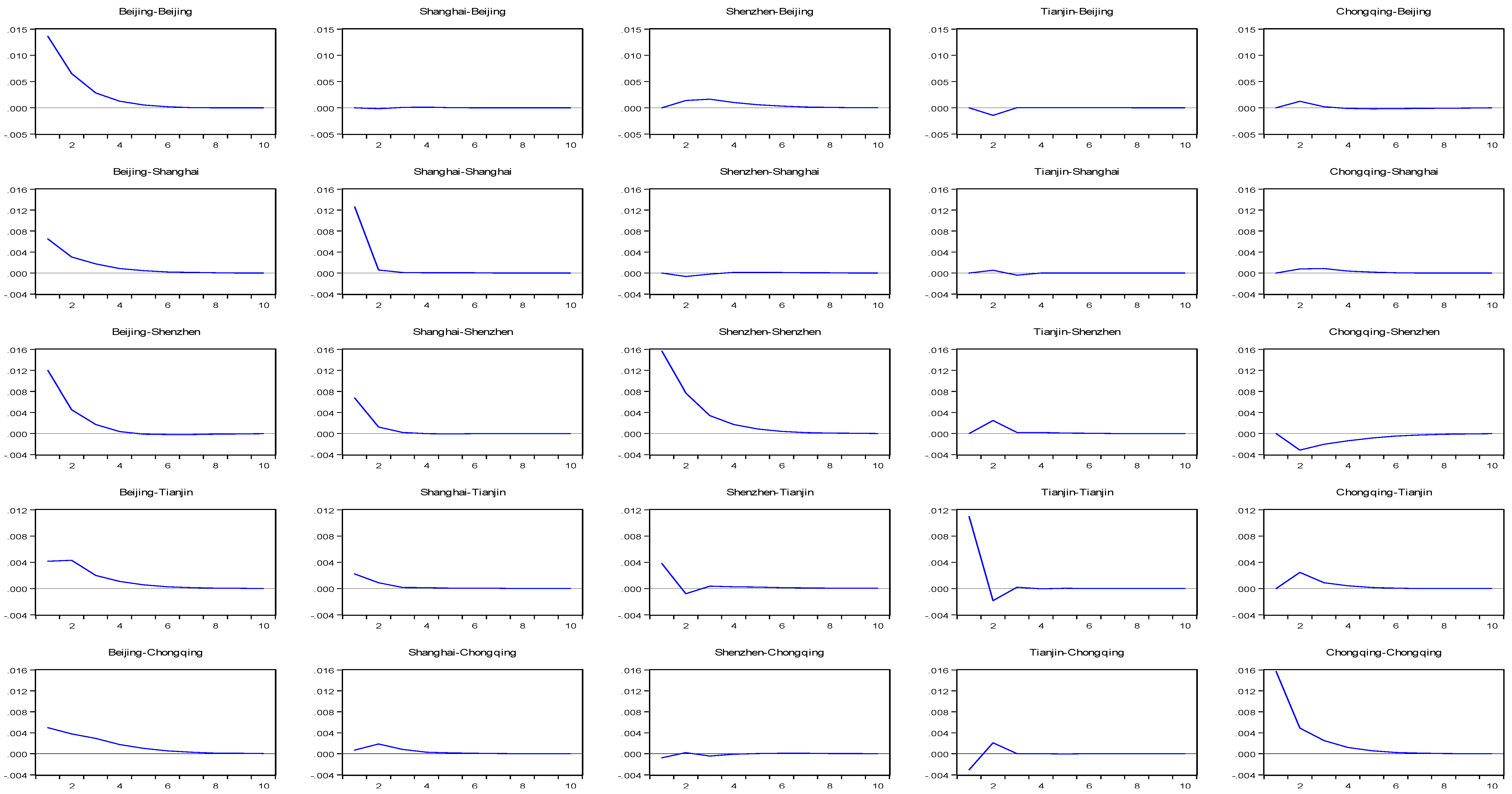
Figure 1. Impulse response function obtained from the VAR model using the all house price returns.
Sustainability 10 02386 g001
Figure 2. Impulse response function obtained from the VAR model using the two house price returns.
Sustainability 10 02386 g002
Figure 3. Volatility impulse response function obtained from the VAR-MGARCH model.
Sustainability 10 02386 g003
Figure 4. Volatility impulse response function obtained from the VAR-MGARCH model using data before the GFC.
Sustainability 10 02386 g004
Figure 5. Volatility impulse response function obtained from the VAR-MGARCH model using data after the GFC.
Sustainability 10 02386 g005
Figure 6. Shocks from macroeconomics.
Sustainability 10 02386 g006
Table 1. Statistics and simple tests.
Growth RateBeijingShanghaiShenzhenTianjinChongqingM2SRCPILoan
Mean0.00760.00710.00740.00490.00410.0126−0.00150.00000.0138
S.D.0.01550.01450.02330.01370.01840.01060.02190.00610.0186
Skewness−1.0443−1.1856−1.68590.2647−0.05210.8063−3.3386−0.4035−0.0560
Kurtosis14.259219.940834.54839.57317.46095.118226.12664.796011.7206
J-B1081.83502414.05308304.9580358.7539164.261358.46934780.253031.9846627.5103
(0.0000)(0.0000)(0.0000)(0.0000)(0.0000)(0.0000)(0.0000)(0.0000)(0.0000)
PP−8.8642−12.4901−8.9398−14.5283−9.9034−15.5449−10.3162−13.6745−7.4736
(0.0000)(0.0000)(0.0000)(0.0000)(0.0000)(0.0000)(0.0000)(0.0000)(0.0000)
LB Q(5)108.3823.28651.97636.31050.83835.02947.55210.542300.980
(0.0000)(0.0000)(0.0000)(0.0000)(0.0000)(0.0000)(0.0000)(0.0000)(0.0000)
LB Q(10)121.2224.72356.15050.75054.14162.48951.85321.869535.450
(0.0000)(0.0000)(0.0000)(0.0000)(0.0000)(0.0000)(0.0000)(0.0000)(0.0000)
Notes: This table represents describe statistics and simple tests for the property of using series. The data included the house price returns of the five major cities, and the growth rates of money supply, short-term rate, CPI and loan balance. The entry in parenthesis stands for the p-value.
Table 2. Vector autoregression estimates using the five cities’ house price returns.
CitesBeijingShanghaiShenzhenTianjinChongqing
Beijing t 1 0.4081 *** (4.7301)0.2046 ** (2.2789)0.0395 (0.2988)0.2652 *** (3.3372)0.0637 (0.6000)
Shanghai t 1 −0.0646 (−0.7881)0.0612 (0.7173)−0.1590 (−1.2647)0.0915 (1.2125)0.1028 (1.0189)
Shenzhen t 1 0.1204 (2.2450)−0.0534 (−0.9561)0.4425 *** (5.3802)−0.0133 (−0.2685)−0.0383 (−0.5795)
Tianjin t 1 −0.1103 (−1.3492)0.0615 (0.7219)0.1686 (1.3447)−0.1263 (−1.6760)0.2783 *** (2.7648)
Chongqing t 1 0.0775 (1.3521)0.0499 (0.8366)−0.2006 ** (−2.2816)0.1566 *** (2.9638)0.3127 *** (4.4297)
Constant 0.0043 *** (3.8265)0.0049 *** (4.2222)0.0050 ** (2.9158)0.0023 (2.2216)0.0005 (0.3531)
Log likelihood2852.157
Akaike information criterion−28.6513
Schwarz criterion−28.1514
Notes: The lag length of the VAR model is selected by using the Schwarz information criterion. The entry in parenthesis stands for the t-statistic. The symbol ** and *** denotes significant at the 5% and 1% level.
Table 3. Interaction between cities.
Variable: r x 1
Variable: r x 2
Beijing-ShanghaiBeijing-ShenzhenBeijing-TianjinBeijing-ChongqingShanghai-ShenzhenShanghai-TianjinShanghai-ChongqingShenzhen-TianjinShenzhen-ChongqingTianjin-Chongqing
Dependent Variable: r x 1
r x 1 , t 1 0.4800 ***
(6.6076)
0.3956 ***
(5.1972)
0.5082 ***
(7.2067)
0.4412 ***
(6.5213)
0.1512
(1.8604)
0.1249
(1.6467)
0.1340
(1.8443)
0.3956 ***
(5.6230)
0.4487 ***
(6.9676)
0.0239
(0.3518)
r x 2 , t 1 −0.0211
(−0.2721)
0.0881
(1.7419)
−0.0961
(−1.2050)
0.0680
(1.1931)
0.0153
(0.3022)
0.1100
(1.3694)
0.0927
(1.6190)
0.1336
(1.1161)
−0.2097 ***
(−2.5706)
0.2426 ***
(4.7880)
Constant 0.0041 ***
(3.6396)
0.0039 ***
(3.6289)
0.0042 ***
(3.8323)
0.0040 ***
(3.6450)
0.0058 ***
(5.0923)
0.0056 ***
(4.8504)
0.0057 ***
(4.9963)
0.0039 ***
(2.3877)
0.0050 ***
(3.1589)
0.0038 ***
(3.7649)
Dependent Variable: r x 2
r x 1 , t 1 0.2080 ***
(2.7904)
−0.0571
(−0.4837)
0.3645 ***
(5.5396)
0.1906 **
(2.2685)
−0.1716
(−1.4403)
0.2393 ***
(3.3779)
0.1991 **
(2.3024)
0.1055 ***
(2.3345)
0.0772
(1.4574)
0.3214 ***
(3.6851)
r x 2 , t 1 0.0546
(0.6851)
0.4479 ***
(5.7044)
−0.1305
(−1.7537)
0.3065 ***
(4.3332)
0.4789 ***
(6.4629)
−0.0404
(−0.5386)
0.3252 ***
(4.7738)
−0.0174
(−0.2266)
0.3511 ***
(5.2316)
0.3428 ***
(5.2818)
Constant 0.0051 ***
(4.3663)
0.0046 ***
(2.7227)
0.0028 ***
(2.6783)
0.0014
(1.0035)
0.0051 ***
(3.0593)
0.0034 ***
(3.1386)
0.0013
(0.9738)
0.0042 ***
(3.9959)
0.0021
(1.5733)
0.0011
(0.8420)
Log likelihood1148.0711081.5841158.6871097.8181070.5191142.6391086.4011064.0981009.2421105.320
A. I. C.−11.5946−10.9196−11.7024−11.0845−10.8073−11.5395−10.9685−10.7421−10.1852−11.1606
S. C.−11.4946−10.8196−11.6024−10.9844−10.7073−11.4395−10.8686−10.6421−10.0852−11.0606
Notes: r x represents the city’s house price returns. The entry in parenthesis stands for the t-statistic. The symbol ** and *** denotes significant at the 5% and 1% level.
Table 4. VAR-MGARCH model.
r x 1 :
r x 2 :
Beijing-ShanghaiBeijing-ShenzhenBeijing-TianjinBeijing-ChongqingShanghai-Shenzhen
Mean model: r x 1
r x 1 , t 1 0.3088 ***0.5207 ***0.6504 ***0.5267 ***0.4577 ***
r x 2 , t 1 0.2154 ***0.2066 **−0.02850.0897−0.0037
Constant 0.01100.08350.2417 **0.3049 ***0.2121 ***
Mean model: r x 2
r x 1 , t 1 0.0663−0.08640.2709 ***0.1344 **−0.0342
r x 2 , t 1 0.2737 ***0.5731 ***0.1911 **0.4838 ***0.5195 ***
Constant 0.5066 ***0.2799 ***0.11590.05890.2406 ***
a 11 1.5777 ***−0.9708 ***0.3064 ***0.21050.8481 ***
a 12 0.5988 ***−2.0079 ***−0.0505−0.08390.5352 ***
a 21 −0.6423 ***0.9186 ***0.12410.14970.5491 ***
a 22 −0.6418 ***1.6348 ***0.5332 ***0.5469 ***2.0986 ***
b 11 −0.2520 ***−0.4064 ***0.07530.18290.7394 ***
b 12 0.0790−0.2831 **−0.3175−0.3744 ***−0.2217
b 21 −0.13270.0138−0.2113−0.0704−0.3071 ***
b 22 −0.18610.2959 ***0.7664 ***0.8486 ***0.0843
c 11 0.3356 **0.6891 ***1.2492 ***1.2649 ***0.4490 **
c 21 0.3277−0.4475 ***0.5343 ***0.4463 ***0.4556 **
c 22 1.1160 ***0.00000.2745 ***0.0000−0.3513
Log Likelihood−635.5467−672.5319−613.9682−655.0680−680.1842
Notes: r x represents the city’s house price returns. a i i , b i i , c i i are volatility-related coefficients. The entry in parenthesis stands for the p-value. The symbol ** and *** denotes significant at the 5% and 1% level.
Table 5. House price returns of Beijing and macroeconomic variables.
x 1 : r x
x 2 : r M a c
Beijing- M 2 Beijing- S R Beijing- C P I Beijing- L o a n
Mean model: r x
r x , t 1 0.6025 ***0.5677 ***0.5490 ***0.4538 ***
r M a c , t 1 0.07740.02790.3804 **0.0348
Constant 0.14080.2797 **0.2001 ***0.3159 ***
Mean model: r M a c
r x , t 1 −0.04750.2127 **0.0666 **−0.0020
r M a c , t 1 −0.1707 **0.27790.10510.7813 ***
Constant 1.5084 ***−0.2055−0.1265 ***0.2437 ***
a 11 0.2776 ***0.2920 **0.6404 ***−0.2470 **
a 12 −0.08490.12320.04000.0178
a 21 0.03810.00201.5065 ***0.0419
a 22 0.4402 ***0.6955 ***0.09411.0802 ***
b 11 0.1959−0.1339−0.05150.3615
b 12 0.2463−0.33690.04750.5652 ***
b 21 0.1161−0.01870.8198 ***−0.0093
b 22 0.7587 ***0.4822 ***−0.7586 ***0.0092
c 11 1.2640 ***1.2899 ***0.6123 ***1.2394 ***
c 21 −0.13280.06830.392 ***−0.1307
c 22 0.34071.1827 ***0.00010.0000
Log Likelihood−617.6144−727.1466−499.0443−649.6231
Notes: r x represents the city’s house price returns. r M a c denotes the growth rate of the macroeconomic variable, including money supply, short-term rate, CPI and loan balance. a i i , b i i , c i i are volatility-related coefficients. The symbol ** and *** denotes significant at the 5% and 1% level.
Table 6. House price returns of Shanghai and macroeconomic variables.
x 1 : r x
x 2 : r M a c
Shanghai- M 2 Shanghai- S R Shanghai- C P I Shanghai- L o a n
Mean model: r x
r x , t 1 0.5452 ***0.1592 ***0.2993 ***0.1406 **
r M a c , t 1 0.0206−0.0106−0.2060.1079
Constant 0.3963 ***0.7144 ***0.4520 ***0.5166 ***
Mean model: r M a c
r x , t 1 −0.00520.08080.0642 **−0.0339
r M a c , t 1 −0.1585 **0.6596 ***0.00690.8278 ***
Constant 1.4253 ***−0.0864−0.03770.2090 ***
a 11 1.1006 ***0.12750.3607 ***−0.0507
a 12 −0.0698−1.0544 ***0.0472−0.4245 ***
a 21 0.2225 **0.1065−2.0562 ***−0.0572
a 22 0.4075 ***1.1876 ***0.14621.1490 ***
b 11 0.1017−0.5294 **−0.23270.0039
b 12 −0.0572−0.0295−0.0991−0.0338
b 21 0.0710.0538−0.39160.0773
b 22 −0.8048 ***0.3836 ***0.7371 ***0.0170
c 11 0.8696 ***1.1839 ***0.5833 ***1.4092 ***
c 21 −0.04550.03690.33550.1372
c 22 0.4573 ***00.1791−0.6115 ***
Log Likelihood−610.0859−688.4462−487.3369−646.4284
Notes: r x represents the city’s house price returns. r M a c denotes the growth rate of the macroeconomic variable, including money supply, short-term rate, CPI and loan balance. a i i , b i i , c i i are volatility-related coefficients. The symbol ** and *** denotes significant at the 5% and 1% level.
Table 7. House price returns of Shenzhen and macroeconomic variables.
x 1 : r x
x 2 : r M a c
Shenzhen- M 2 Shenzhen- S R Shenzhen- C P I Shenzhen- L o a n
Mean model: r x
r x , t 1 0.4951 ***0.6939 ***0.4958 ***0.2986 ***
r M a c , t 1 −0.1392 ***−0.0067−0.2706 **−0.2638 ***
C o n s t a n t 0.4096 ***0.2479 ***0.2420 ***0.9387 ***
Mean model: r M a c
r x , t 1 0.03150.06500.0371 **0.0278
r M a c , t 1 −0.10630.2469 ***0.04280.6578 ***
C o n s t a n t 1.3513 ***0.0038−0.02210.2702 ***
a 11 2.2748 ***2.2638 ***1.3586 ***1.6001 ***
a 12 −0.08860.09970.0827 **−0.2190 ***
a 21 −0.2766 ***0.1116 **−1.6219 ***−0.3830 ***
a 22 0.1819 **0.7157 ***0.06021.1610 ***
b 11 −0.00500.0911−0.0175−0.1515
b 12 0.0346−0.3333 ***−0.0589 **−0.1825 ***
b 21 −0.14530.05200.30360.0338
b 22 0.9353 ***0.6368 ***0.9571 ***−0.2530
c 11 0.4986 ***0.6926 ***0.6556 ***1.0392 ***
c 21 0.3073 **0.1434−0.14540.2695 **
c 22 0.00000.6859 ***0.00000.6501 ***
Log Likelihood−663.0777−768.3753−526.4602−702.1470
Notes: r x represents the city’s house price returns. r M a c denotes the growth rate of the macroeconomic variable, including money supply, short-term rate, CPI and loan balance. a i i , b i i , c i i are volatility-related coefficients. The symbol ** and *** denotes significant at the 5% and 1% level.