Contrasted Effects of Relative Humidity and Precipitation on Urban PM_2.5 Pollution in High Elevation Urban Areas

Abstract

Levels of urban pollution can be influenced largely by meteorological conditions and the topography of the area. The impact of the relative humidity (RH) on the daily average PM_2.5 concentrations was studied at several sites in a mid-size South American city at a high elevation over the period of nine years. In this work, we show that there is a positive correlation between daily average urban PM_2.5 concentrations and the RH in traffic-busy central areas, and a negative correlation in the outskirts of the city in more industrial areas. While in the traffic sites strong events of precipitation (≥9 mm) played a major role in PM_2.5 pollution removal, in the city outskirts, the PM_2.5 concentrations decreased with increasing RH independently of rain accumulation. Increasing PM_2.5 concentrations are to be expected in any highly motorized city where there is high RH and a lack of strong precipitation, especially in rapidly growing and developing countries with high motorization due to poor fuel quality. Finally, two models, based on a logistic regression algorithm, are proposed to describe the effect of rain and RH on PM_2.5, when the source of pollution is traffic-based vs. industry-based.

1. Introduction

The cities of the developing world with populations greater than 100,000 dominate the list of urban areas at high elevations (>2000 m.a.s.l.). Small- and mid-size cities (<5 million people) in these regions are currently among the fastest growing areas in the world and are often more polluted than major urban conglomerations [1,2]. Most often, this is due to a lack of strict regulation, inappropriate urban planning, the age of the motorized fleet or engine technology, and poor quality fuel [3,4]. In these areas, traffic is frequently a major source of ambient PM_2.5 (particulate matter with aerodynamic diameter less than 2.5 µm) pollution, and can account for as much as 37% of observed levels [5].

High elevation urban areas are conditioned to different meteorology compared to low elevation regions. At high altitude, more intense solar radiation causes more active photochemistry and a high diurnal temperature variation. Even at tropical and subtropical climate zones, temperature is lower compared to the same latitude at sea level. Moreover, relative humidity (RH) at high altitude varies during the day depending on temperature and formation of clouds. The same RH at higher elevation, however, contains less water vapor. In addition, atmospheric pressure decreases with elevation, causing lower air density and less oxygen.

It has been shown that levels of urban pollution can be strongly influenced by both meteorological conditions and the topography of the area [6]. Temperature, wind speed, and precipitation may have negative effects on the PM_2.5 concentrations due to better diffusion and wet deposition [7,8,9,10,11,12,13]. However, a study in the Chinese city Zanzhou (elevation 1520 m.a.s.l.), indicates that precipitation scavenging effect on different size PM is dependent on the strength and accumulation of precipitation [14]. Several studies conclude that an increase in the RH reduces urban PM_2.5 pollution [11,15,16,17,18,19,20]. In contrast, others indicate a positive effect, especially during episodes of high pollution in wintertime [21,22,23]. Those periods are known to have low precipitation. Some studies show how the concentrations of PM_2.5 of different chemical composition increase as a function of the RH due to the aqueous-phase reactions (secondary inorganic species) and gas-particle partitioning associated with water uptake (secondary organic aerosol) [21,24,25]. These effects could explain a fraction of the enhanced aerosol formation due to increased RH. However, most of the studies carried out on an urban scale are limited to short-term investigations of regions that use cleaner fuels in low elevation cities.

Decades of research at the vehicle scale point out both RH and elevation enhanced particulate emissions from internal combustion engines [26,27,28,29]. Increased RH results in lower temperature due to the increased heat capacity of the cylinder air charge [26]. Furthermore, an increase in soot particles, hydrocarbons, and other unburnt fuel compounds that form primary particles is also due to higher atmospheric moisture content reducing the air density at intake and causing a decrease in oxygen content, influencing the air-to-fuel ratio of the combust mixture [9,28]. Increased elevation also reduces ambient temperature, air density and the oxygen available in the air. A study on diesel emissions at high elevation showed that particulate matter emissions at elevations between sea level and 1000 m.a.s.l., and sea level and 3200 m.a.s.l. increased by 142.3% and 203.5%, respectively [30]. It was further concluded that smoke emissions in heavy-duty diesel engines increase at higher elevations [31]. There are reports proving RH effects on the post-combustion, dilution, and secondary aerosol processes of PM formation [8,9,10,32,33,34]. While the impact of RH or elevation on gasoline engine emissions has not been explored, it may be assumed that high RH and elevation have a similar effect on both gasoline and diesel engine PM emissions due to incomplete combustion [29]. However, it was recently concluded that gasoline cars produce more carbonaceous particulate matter than modern filter-equipped diesel cars [35].

Although several studies show the increased emissions at the vehicle scale, there is a general lack of studies on the effect of RH on PM_2.5 pollution in high elevation cities at the urban scale [36]. Moreover, most of the existing studies on PM_2.5 pollution focus on the large cities or megacities where the sulfur content in fuel is often strictly regulated [37]. The impact of RH on internal engine combustion could be more of concern at high elevations and more so in the developing countries where fuels with a high sulfur content are more common. This means that traffic related pollution could become more of an issue in those countries during episodes of high relative humidity. While sulfur content in the developed world is under 10–15 ppm, corresponding to Euro 6 vehicle technologies, developing countries are circulating much higher sulfur content fuels corresponding to Euro 0–3 vehicle technologies. For example, in 2017, rapidly growing Ecuador, with fuels with sulfur content over 500 ppm, passed a new regulation of Euro 3, which was the standard implemented in Europe in the 1990s. Quito, the capital of Ecuador, therefore offers a perfect site for studying mid-sized cities at high elevations that violate the World Health Organization (WHO, Geneva, Switzerland) and national annual PM_2.5 standards due to transport-related (80%) PM_2.5 emissions [36,38]. Quito also has relatively consistent weather conditions throughout the year, with the only exception of the seasonal variation of RH and rain accumulation (the rainy and dry seasons). The goal of this work was to study the contrasting effect of RH and precipitation on fine urban particulate pollution in a high elevation mid-size city, using Quito as the model. We first searched for more traffic-busy urban areas and focused on how the rain might affect the relationship between the RH and PM_2.5 concentrations. We then separated the rain component from the dataset to better illustrate the RH impact on different PM_2.5. Finally, models based on logistic regression were proposed to describe the contrasted effect of rain and RH on urban PM_2.5 pollution in different parts of the city.

2. Materials and Methods

2.1. Site Description

Quito is among the top five most populated cities at high elevations in the world. It stretches north to south over a broad slope of the Pichincha volcano (the summit of which is 4800 m.a.sl.), which forms part of the Andes, and has an average elevation of 2815 m.a.s.l. [39]. The city is currently experiencing expansion of the metropolitan area (4218 km²) and is host to a population of 2,239,191 according to the last census taken in 2010 [40]. The city extends over several terraces that vary in elevation between 2700 and 3000 m.a.s.l., and expands through to the surrounding valleys that stand at 2300–2450 m.a.s.l. A motorized fleet of around 0.5 million vehicles creates serious rush-hour problems due to the limitations placed on the city sprawl as a result of the complex topography. Due to its location on the Equator, the solar height at midday is between 66.5 and 90 degrees throughout the year with high solar intensity levels. However, thanks to the elevation, it has a spring-like climate all-year round with an average temperature of 14.5 °C [39]. Quito is located in a high-elevation tropical region and consequently has two seasons: dry (June-August, with average rainfall of around 14 mm/month) and rainy (September-May, with average rainfall of 59 mm/month) with most of the rainfall occurring in afternoons.

PM_2.5 pollution in the city can be generated by different sources such as traffic, wood combustion, mining, industrial parks, and thermoelectric power plants (Figure 1). The center of Quito is predominated by residential areas with heavy vehicular traffic. The industrial parks are mainly located in the northern and southern outskirts of the city. In addition, in the surroundings of the city, there are quarry areas that produce aggregates for the building construction sector and two thermal power stations.

2.2. Instrumentation and Data Analysis

To account for the variability of the Quito’s complex terrain, air quality and meteorological data were collected from five sites over a period of nine years, 2007–2016. The selected sites vary by elevation and vehicle traffic densities. Two northern sites (Cotocollao (elevation 2739 m.a.s.l., coordinates 78°29′50″ W, 0°6′28″ S) and Carapungo (elevation 2660 m.a.s.l., coordinates 78°26′50″ W, 0°5′54″ S)), one central site (Belisario, (elevation 2835 m.a.s.l, coordinates 78°29′24″ W, 0°10′48″ S)), and two southern sites (Camal (elevation 2840 m.a.s.l., coordinates 78°30′36″ W, 0°15′00″ S) and Chillos (elevation 2453 m.a.s.l., coordinates 78°27′36″ W, 0°18′00″ S)) were studied (see Figure 1). The latter site has only been operating since 2014. The measurement stations were located on the roofs of relatively tall buildings in line with the criteria for air quality monitoring set by the Environmental Protection Agency of the United States (USEPA, Washington, DC, USA).

For PM_2.5 concentration data, Thermo Scientific FH62C14-DHS continuous ambient particulate monitor 5014i was used based on beta rays’ attenuation method (EPA No. EQPM-0609-183). Crucial to this study is that the sample was drawn at a flow rate of 16.67 L/min through a heated sampling tube, the purpose of which was to reduce particle-bound water and to decrease the margin of error in the measurement due to RH. The RH threshold of the sampling tube heater was 35%. For SO₂ concentration data collection, ThermoFisher Scientific (Waltham, MA, USA) 43i high level SO₂ analyzer based on ultraviolet florescence (EPA No. EQSA-0486-060) was used. For concentration data collection, ThermoFisher Scientific 49i ozone analyzer based on ultraviolet absorption (EPA No. EQOA-0880-047) was used. For NO₂ concentration data collection, ThermoFisher Scientific 42i NO_x analyzer based on a chemiluminescence method (EPA No. RFNA-1289-074) was used. Finally, for CO concentration data collection, ThermoFisher Scientific 48i based on infrared absorption (EPA No. RFCA-0981-054) was used. All meteorological parameters were measured using Vaisala WXT536 instrumentation. Kipp&Zonnen (Delft, The Netherlands) pyrometer was used to measure global solar radiation.

Carto Enterprise map application (www.carto.com) was used to produce the map of Quito. Igor Pro (Wavemetrics) and Microsoft Excel (MS Office) software applications were used to perform daily data correlation analyses and descriptive statistics. The air pollution and meteorological data were compiled as 3-h (0:00–3:00, 3:00–6:00, 6:00–9:00, 9:00–12:00, 12:00–15:00, 15:00–18:00, 18:00–1:00 and 21:00–24:00) and 24-h averages. Python statistics module of the SciPy library was used to carry out the inferential statistics (i.e., interaction test). A data mining approach was applied to classify the PM_2.5 concentrations between the values above and below long-term median in relation to RH and precipitation. The classification of data was obtained through a machine learning algorithm called logistic regression. The Scikit-learn machine learning library for Python programming language was used to implement the classifications and build the respective models.

3. Results and Discussion

3.1. Long Term Air Quality and Meteorological Data Analysis

The statistical analyses of daily data show that the 2007–2016 average RH for central Quito is relatively high at 69.9%, and that the annual average PM_2.5 concentration is elevated at 17.1 ± 6.05 µg/m³ (median 17.0 µg/m³). The area has been undergoing some changes in climate, with ambient temperature increase from 13.5 °C to 14.8 °C in the past decade. In the same period, the annual RH average steadily decreased from about 76% to 64% in all the monitored sites. The overall decreasing trend in PM_2.5 concentrations is registered in Belisario and Camal districts by 12.6% and 2.8%, respectively, while, in northern Cotocollao and Carapungo, we see a steady increase by 12.9% and 11.4%, respectively. 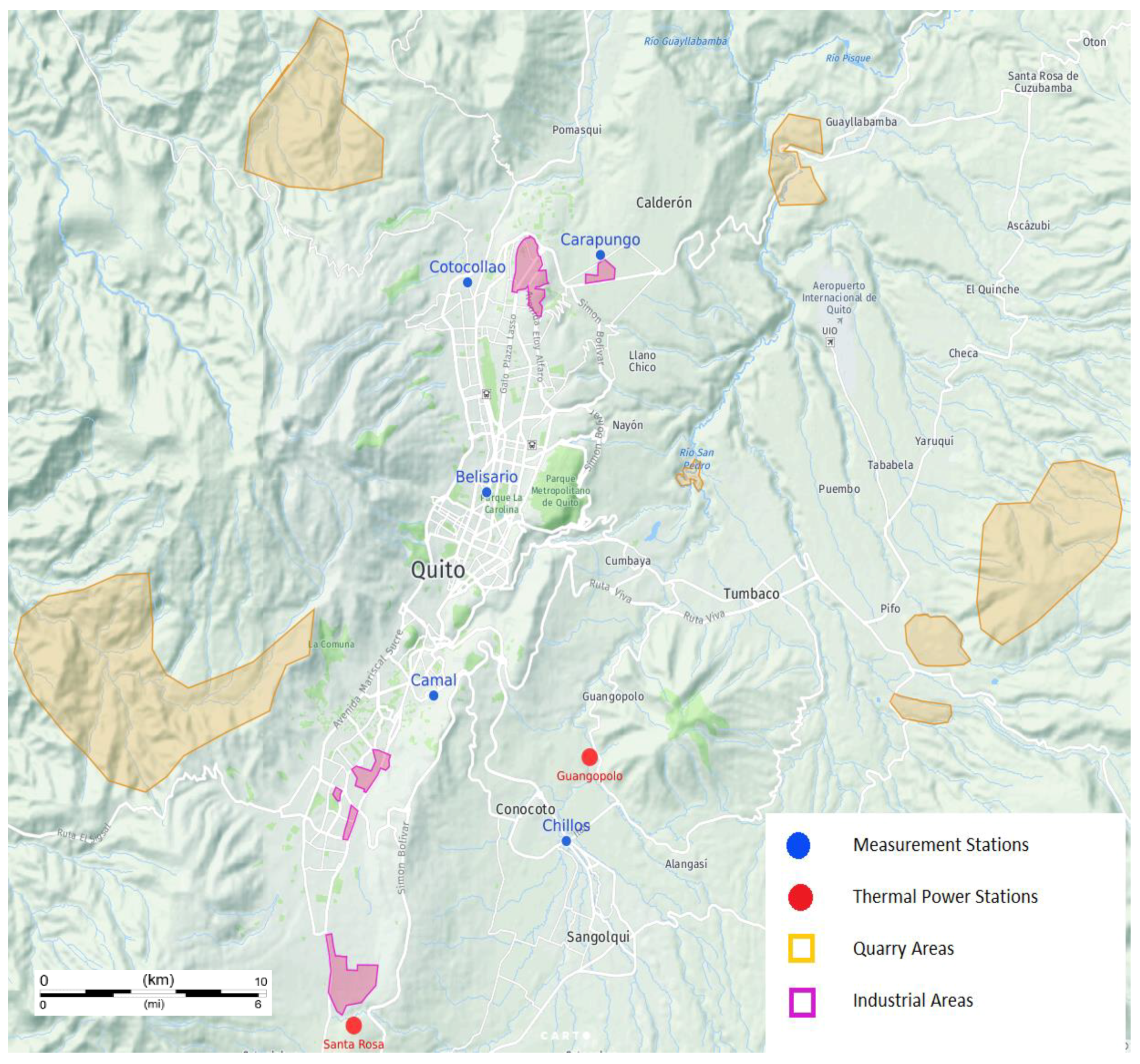As reported in an earlier study, these changes in annual concentrations are due to the implemented fuel and traffic regulations in the city of Quito and all of Ecuador, and a continued growth of the city at the outskirts [4]. The gaseous criteria pollutants tend to be elevated depending on the location or season. For example, ozone tends to exceed WHO’s recommendations in September due to the high UV radiation (dry season, no cloud cover combined with direct sun angle), or SO₂ is elevated in the Chillos site located close to the thermoelectric power plant (see Figure 1).

Although the city suffers from long-term elevated PM_2.5 pollution, mostly due to mobile sources coming from poor quality fuels and old technologies [4,36], it has limited resources to study chemical composition of particulate matter. To confirm the PM_2.5 correlation with other common mobile source emissions in an urban area, correlation analyses of PM_2.5 concentration data and CO, NO₂, SO₂, and O₃ concentrations was performed for all the sites (

Table A1. Belisario correlation analysis of all the meteorological and pollution parameters for 2007–2016 (values in bold α = 0.05). RH, relative humidity; Temp, temperature; Pres, atmospheric pressure; WS, wind speed; WD, wind direction; SR, solar radiation.

Variables	PM2.5	RH	Rain	Temp	Pres	WS	WD	SR	O3	SO2	NO2	CO
PM2.5	1	0.46	0.02	−0.27	−0.03	−0.45	−0.16	−0.23	−0.26	0.52	0.67	0.56
RH	0.46	1	0.42	−0.75	−0.01	−0.77	−0.45	−0.68	−0.65	0.25	0.39	0.48
Rain	0.02	0.42	1	−0.45	0.04	−0.25	−0.1	−0.32	−0.18	0.03	0.15	0.27
Temp	−0.27	−0.75	−0.45	1	−0.06	0.59	0.23	0.68	0.41	−0.28	−0.4	−0.46
Pres	−0.03	−0.01	0.04	−0.06	1	0.03	−0.01	0	0.03	0.02	−0.02	0.01
WS	−0.45	−0.77	−0.25	0.59	0.03	1	0.23	0.63	0.65	−0.33	−0.44	−0.43
WD	−0.16	−0.45	−0.1	0.23	−0.01	0.23	1	0.2	0.21	−0.09	−0.03	−0.14
SR	−0.23	−0.68	−0.32	0.68	0	0.63	0.2	1	0.56	−0.19	−0.31	−0.39
O3	−0.26	−0.65	−0.18	0.41	0.03	0.65	0.21	0.56	1	−0.28	−0.19	−0.37
SO2	0.52	0.25	0.03	−0.28	0.02	−0.33	−0.09	−0.19	−0.28	1	0.48	0.54
NO2	0.67	0.39	0.15	−0.4	−0.02	−0.44	−0.03	−0.31	−0.19	0.48	1	0.58
CO	0.56	0.48	0.27	−0.46	0.01	−0.43	−0.14	−0.39	−0.37	0.54	0.58	1

,

Table A2. Belisario correlation analysis of all the meteorological and pollution parameters during all the days with no rain events for 2007–2016 (values in bold α = 0.05). RH, relative humidity; Temp, temperature; Pres, atmospheric pressure; WS, wind speed; WD, wind direction; SR, solar radiation.

Variables	PM2.5	RH	Temp	Pres	WS	WD	SR	O3	SO2	NO2	CO
PM2.5	1	0.62	−0.41	−0.04	−0.53	−0.29	−0.27	−0.27	0.56	0.65	0.61
RH	0.62	1	−0.59	−0.05	−0.75	−0.52	−0.54	−0.65	0.43	0.4	0.48
Temp	−0.41	−0.59	1	−0.04	0.48	0.23	0.51	0.28	−0.41	−0.39	−0.37
Pres	−0.04	−0.05	−0.04	1	0.06	−0.01	0.04	0.05	−0.01	−0.04	−0.04
WS	−0.53	−0.75	0.48	0.06	1	0.27	0.53	0.65	−0.45	−0.46	−0.44
WD	−0.29	−0.52	0.23	−0.01	0.27	1	0.2	0.22	−0.18	−0.08	−0.2
SR	−0.27	−0.54	0.51	0.04	0.53	0.2	1	0.5	−0.26	−0.26	−0.29
O3	−0.27	−0.65	0.28	0.05	0.65	0.22	0.5	1	−0.34	−0.16	−0.32
SO2	0.56	0.43	−0.41	−0.01	−0.45	−0.18	−0.26	−0.34	1	0.49	0.57
NO2	0.65	0.4	−0.39	−0.04	−0.46	−0.08	−0.26	−0.16	0.49	1	0.57
CO	0.61	0.48	−0.37	−0.04	−0.44	−0.2	−0.29	−0.32	0.57	0.57	1

,

Table A3. Cotocollao correlation analysis of all the meteorological and pollution parameters for 2007–2016 (values in bold α = 0.05). RH, relative humidity; Temp, temperature; Pres, atmospheric pressure; WS, wind speed; WD, wind direction; SR, solar radiation.

Variables	PM2.5	RH	Rain	Temp	Pres	WS	WD	SR	O3	SO2	NO2	CO
PM2.5	1	0.06	−0.13	0.04	−0.08	−0.27	0.09	0.05	0.04	0.31	0.5	0.3
RH	0.06	1	0.23	−0.68	0.17	−0.69	−0.32	−0.48	−0.53	−0.09	0.01	0.14
Rain	−0.13	0.23	1	−0.29	0.25	−0.09	−0.1	−0.18	−0.04	0.04	0.02	0.1
Temp	0.04	−0.68	−0.29	1	−0.31	0.48	0.18	0.54	0.31	0.01	−0.17	−0.16
Pres	−0.08	0.17	0.25	−0.31	1	−0.11	−0.07	−0.23	0.05	0.21	0.05	0.11
WS	−0.27	−0.69	−0.09	0.48	−0.11	1	0.09	0.5	0.49	−0.21	−0.25	−0.28
WD	0.09	−0.32	−0.1	0.18	−0.07	0.09	1	0.27	0.1	0.08	0.12	0.11
SR	0.05	−0.48	−0.18	0.54	−0.23	0.5	0.27	1	0.38	−0.08	−0.11	−0.19
O3	0.04	−0.53	−0.04	0.31	0.05	0.49	0.1	0.38	1	−0.01	0.11	−0.12
SO2	0.31	−0.09	0.04	0.01	0.21	−0.21	0.08	−0.08	−0.01	1	0.35	0.29
NO2	0.5	0.01	0.02	−0.17	0.05	−0.25	0.12	−0.11	0.11	0.35	1	0.52
CO	0.3	0.14	0.1	−0.16	0.11	−0.28	0.11	−0.19	−0.12	0.29	0.52	1

,

Table A4. Cotocollao correlation analysis of all the meteorological and pollution parameters during all the days with no rain events for 2007–2016 (values in bold α = 0.05). RH, relative humidity; Temp, temperature; Pres, atmospheric pressure; WS, wind speed; WD, wind direction; SR, solar radiation.

Variables	PM2.5	RH	Temp	Pres	WS	WD	SR	O3	SO2	NO2	CO
PM2.5	1	0.3	−0.19	−0.03	−0.39	0.02	−0.05	−0.03	0.26	0.48	0.31
RH	0.3	1	−0.56	0.1	−0.72	−0.23	−0.35	−0.54	0.06	−0.01	0.15
Temp	−0.19	−0.56	1	−0.26	0.46	0.06	0.37	0.24	−0.13	−0.2	−0.15
Pres	−0.03	0.1	−0.26	1	−0.08	0.02	−0.17	0.09	0.23	0.04	0.06
WS	−0.39	−0.72	0.46	−0.08	1	0.04	0.45	0.51	−0.29	−0.26	−0.29
WD	0.02	−0.23	0.06	0.02	0.04	1	0.2	0.06	0.02	0.09	0.1
SR	−0.05	−0.35	0.37	−0.17	0.45	0.2	1	0.35	−0.17	−0.08	−0.18
O3	−0.03	−0.54	0.24	0.09	0.51	0.06	0.35	1	−0.08	0.13	−0.12
SO2	0.26	0.06	−0.13	0.23	−0.29	0.02	−0.17	−0.08	1	0.34	0.27
NO2	0.48	−0.01	−0.2	0.04	−0.26	0.09	−0.08	0.13	0.34	1	0.49
CO	0.31	0.15	−0.15	0.06	−0.29	0.1	−0.18	−0.12	0.27	0.49	1

,

Table A5. Chillos correlation analysis of all the meteorological and pollution parameters for 2007–2016 (values in bold α = 0.05). RH, relative humidity; Temp, temperature; Pres, atmospheric pressure; WS, wind speed; WD, wind direction; SR, solar radiation.

Variables	PM2.5	RH	Rain	Temp	Pres	WS	WD	SR	O3	SO2	NO2	CO
PM2.5	1	0.24	0.06	−0.17	−0.07	−0.33	0.05	−0.07	−0.09	0.4	0.52	0.38
RH	0.24	1	0.26	−0.66	0.17	−0.66	0.56	−0.62	−0.36	0.39	0.35	0
Rain	0.06	0.26	1	−0.32	0.11	−0.18	0.01	−0.16	−0.02	0.03	0.35	0.1
Temp	−0.17	−0.66	−0.32	1	−0.22	0.55	−0.26	0.59	0.19	−0.11	−0.39	−0.07
Pres	−0.07	0.17	0.11	−0.22	1	−0.05	−0.03	−0.2	−0.09	−0.07	0.2	−0.09
WS	−0.33	−0.66	−0.18	0.55	−0.05	1	−0.29	0.53	0.36	−0.26	−0.47	−0.26
WD	0.05	0.56	0.01	−0.26	−0.03	−0.29	1	−0.33	−0.05	0.29	0	−0.27
SR	−0.07	−0.62	−0.16	0.59	−0.2	0.53	−0.33	1	0.37	−0.15	−0.19	−0.05
O3	−0.09	−0.36	−0.02	0.19	−0.09	0.36	−0.05	0.37	1	−0.29	−0.05	−0.22
SO2	0.4	0.39	0.03	−0.11	−0.07	−0.26	0.29	−0.15	−0.29	1	0.38	0.03
NO2	0.52	0.35	0.35	−0.39	0.2	−0.47	0	−0.19	−0.05	0.38	1	0.35
CO	0.38	0	0.1	−0.07	−0.09	−0.26	−0.27	−0.05	−0.22	0.03	0.35	1

,

Table A6. Chillos correlation analysis of all the meteorological and pollution parameters during all the days with no rain events for 2007–2016 (values in bold α = 0.05). RH, relative humidity; Temp, temperature; Pres, atmospheric pressure; WS, wind speed; WD, wind direction; SR, solar radiation.

Variables	PM2.5	RH	Temp	Pres	WS	WD	SR	O3	SO2	NO2	CO
PM2.5	1	0.35	−0.22	−0.08	−0.37	0.19	−0.13	−0.09	0.45	0.49	0.3
RH	0.35	1	−0.48	0.05	−0.58	0.68	−0.52	−0.38	0.52	0.22	−0.05
Temp	−0.22	−0.48	1	−0.18	0.41	−0.28	0.46	0.14	−0.14	−0.25	0.03
Pres	−0.08	0.05	−0.18	1	0.04	−0.07	−0.13	−0.05	−0.06	0.18	−0.29
WS	−0.37	−0.58	0.41	0.04	1	−0.41	0.44	0.35	−0.34	−0.36	−0.19
WD	0.19	0.68	−0.28	−0.07	−0.41	1	−0.32	−0.09	0.33	0.06	−0.2
SR	−0.13	−0.52	0.46	−0.13	0.44	−0.32	1	0.36	−0.16	−0.1	−0.06
O3	−0.09	−0.38	0.14	−0.05	0.35	−0.09	0.36	1	−0.32	0.02	−0.21
SO2	0.45	0.52	−0.14	−0.06	−0.34	0.33	−0.16	−0.32	1	0.42	0.08
NO2	0.49	0.22	−0.25	0.18	−0.36	0.06	−0.1	0.02	0.42	1	0.25
CO	0.3	−0.05	0.03	−0.29	−0.19	−0.2	−0.06	−0.21	0.08	0.25	1

,

Table A7. Carapungo correlation analysis of all the meteorological and pollution parameters for 2007–2016 (values in bold α = 0.05). RH, relative humidity; Temp, temperature; Pres, atmospheric pressure; WS, wind speed; WD, wind direction; SR, solar radiation.

Variables	PM2.5	RH	Rain	Temp	Pres	WS	WD	SR	O3	SO2	NO2	CO
PM2.5	1	−0.25	−0.14	0.17	0.08	0.09	−0.16	0.16	0.23	0.36	0.45	0.22
RH	−0.25	1	0.29	−0.69	0.01	−0.44	0.34	−0.46	−0.44	−0.2	−0.24	−0.09
Rain	−0.14	0.29	1	−0.32	0.03	−0.18	0.11	−0.22	−0.07	−0.12	−0.04	0.02
Temp	0.17	−0.69	−0.32	1	−0.04	0.45	−0.27	0.59	0.26	0.12	0.09	−0.06
Pres	0.08	0.01	0.03	−0.04	1	0.11	−0.27	−0.04	0.05	−0.04	0.21	−0.01
WS	0.09	−0.44	−0.18	0.45	0.11	1	−0.46	0.52	0.33	−0.03	0.06	−0.12
WD	−0.16	0.34	0.11	−0.27	−0.27	−0.46	1	−0.2	−0.08	−0.2	−0.44	−0.1
SR	0.16	−0.46	−0.22	0.59	−0.04	0.52	−0.2	1	0.33	0.11	0.09	−0.05
O3	0.23	−0.44	−0.07	0.26	0.05	0.33	−0.08	0.33	1	−0.03	0.14	−0.03
SO2	0.36	−0.2	−0.12	0.12	−0.04	−0.03	−0.2	0.11	−0.03	1	0.56	0.33
NO2	0.45	−0.24	−0.04	0.09	0.21	0.06	−0.44	0.09	0.14	0.56	1	0.45
CO	0.22	−0.09	0.02	−0.06	−0.01	−0.12	−0.1	−0.05	−0.03	0.33	0.45	1

,

Table A8. Carapungo correlation analysis of all the meteorological and pollution parameters during all the days with no rain events for 2007–2016 (values in bold α = 0.05).

Variables	PM2.5	RH	Temp	Pres	WS	WD	SR	O3	SO2	NO2	CO
PM2.5	1	−0.1	−0.01	0.1	0.03	−0.07	0.04	0.18	0.3	0.38	0.21
RH	−0.1	1	−0.6	−0.09	−0.42	0.42	−0.32	−0.46	−0.1	−0.27	−0.12
Temp	−0.01	−0.6	1	0.02	0.37	−0.29	0.45	0.22	0.01	0.05	−0.05
Pres	0.1	−0.09	0.02	1	0.21	−0.32	0.04	0.09	0	0.21	−0.01
WS	0.03	−0.42	0.37	0.21	1	−0.5	0.46	0.31	−0.06	0.09	−0.08
WD	−0.07	0.42	−0.29	−0.32	−0.5	1	−0.22	−0.09	−0.18	−0.41	−0.1
SR	0.04	−0.32	0.45	0.04	0.46	−0.22	1	0.27	0.07	0.07	−0.04
O3	0.18	−0.46	0.22	0.09	0.31	−0.09	0.27	1	−0.03	0.16	−0.01
SO2	0.3	−0.1	0.01	0	−0.06	−0.18	0.07	−0.03	1	0.54	0.3
NO2	0.38	−0.27	0.05	0.21	0.09	−0.41	0.07	0.16	0.54	1	0.45
CO	0.21	−0.12	−0.05	−0.01	−0.08	−0.1	−0.04	−0.01	0.3	0.45	1

,

Table A9. Camal correlation analysis of all the meteorological and pollution parameters for 2007–2016 (values in bold α = 0.05). RH, relative humidity; Temp, temperature; Pres, atmospheric pressure; WS, wind speed; WD, wind direction; SR, solar radiation.

Variables	PM2.5	RH	Rain	Temp	Pres	WS	WD	SR	O3	SO2	NO2	CO
PM2.5	1	−0.15	−0.07	0.04	−0.1	0	−0.13	0.11	0.14	0.33	0.48	0.41
RH	−0.15	1	0.32	−0.67	0.02	−0.44	0.25	−0.46	−0.42	−0.05	−0.09	−0.02
Rain	−0.07	0.32	1	−0.4	−0.17	−0.23	−0.02	−0.28	−0.11	0.08	0.17	0.16
Temp	0.04	−0.67	−0.4	1	0.26	0.46	−0.01	0.61	0.3	−0.21	−0.24	−0.21
Pres	−0.1	0.02	−0.17	0.26	1	0.23	0.53	0.23	0.22	−0.59	−0.57	−0.48
WS	0	−0.44	−0.23	0.46	0.23	1	−0.2	0.54	0.38	−0.2	−0.17	−0.22
WD	−0.13	0.25	−0.02	−0.01	0.53	−0.2	1	0.02	0.12	−0.39	−0.54	−0.35
SR	0.11	−0.46	−0.28	0.61	0.23	0.54	0.02	1	0.39	−0.12	−0.17	−0.17
O3	0.14	−0.42	−0.11	0.3	0.22	0.38	0.12	0.39	1	−0.21	−0.09	−0.15
SO2	0.33	−0.05	0.08	−0.21	−0.59	−0.2	−0.39	−0.12	−0.21	1	0.63	0.53
NO2	0.48	−0.09	0.17	−0.24	−0.57	−0.17	−0.54	−0.17	−0.09	0.63	1	0.69
CO	0.41	−0.02	0.16	−0.21	−0.48	−0.22	−0.35	−0.17	−0.15	0.53	0.69	1

and

Table A10. Camal correlation analysis of all the meteorological and pollution parameters during all the days with no rain events for 2007–2016 (values in bold α = 0.05). RH, relative humidity; Temp, temperature; Pres, atmospheric pressure; WS, wind speed; WD, wind direction; SR, solar radiation.

Variables	PM2.5	RH	Temp	Pres	WS	WD	SR	O3	SO2	NO2	CO
PM2.5	1	0	−0.08	0	−0.02	−0.01	0.05	0.15	0.23	0.38	0.36
RH	0	1	−0.57	0.05	−0.41	0.33	−0.31	−0.44	0	−0.17	−0.06
Temp	−0.08	−0.57	1	0.24	0.36	−0.07	0.46	0.24	−0.25	−0.18	−0.16
Pres	0	0.05	0.24	1	0.23	0.54	0.23	0.22	−0.64	−0.55	−0.44
WS	−0.02	−0.41	0.36	0.23	1	−0.23	0.46	0.38	−0.21	−0.11	−0.15
WD	−0.01	0.33	−0.07	0.54	−0.23	1	−0.02	0.07	−0.38	−0.53	−0.32
SR	0.05	−0.31	0.46	0.23	0.46	−0.02	1	0.34	−0.14	−0.12	−0.14
O3	0.15	−0.44	0.24	0.22	0.38	0.07	0.34	1	−0.22	−0.02	−0.11
SO2	0.23	0	−0.25	−0.64	−0.21	−0.38	−0.14	−0.22	1	0.6	0.52
NO2	0.38	−0.17	−0.18	−0.55	−0.11	−0.53	−0.12	−0.02	0.6	1	0.64
CO	0.36	−0.06	−0.16	−0.44	−0.15	−0.32	−0.14	−0.11	0.52	0.64	1

, Appendix A). The results contrast for different sites. The best linear correlation was obtained at the Belisario site, where daily PM_2.5 concentrations were best correlated with NO₂ (r = 0.67), CO (r = 0.56) and SO₂ (r = 0.52) (Table A1 and Table A2, Appendix A). In addition, stronger ozone effect on weekends [41] and increases in PM_2.5, SO₂, NO₂ and CO concentrations on weekdays were observed in Belisario, Cotocollao and Camal (

Table 1. Air pollution concentration increment (positive values) or reduction (negative values) during the work days (Monday-Friday) if compared to Sundays.

	Belisario	Carapungo	Cotocollao	Camal	Chillos
	%	%	%	%	%
PM2.5	33.26	17.04	25.03	29.40	13.56
O3	−20.56	−6.28	−12.63	−11.74	−6.11
SO2	38.63	25.35	40.68	19.47	15.29
NO2	31.12	19.40	26.27	18.51	13.35
CO	31.82	9.11	13.03	14.56	8.02

). These results support the fact that these contaminants originate highly from anthropogenic sources, with mobile sources being the main contributor. This analysis helped identify more traffic related areas in the city. The Chillos area contains a thermoelectric power plant, the alternators of which are driven by diesel-cycle internal combustion engines powered by diesel, fuel-oil, and reduced crude oil. This thermoelectric plant functions all week long and might not show a weekend drop in pollutant concentrations (Table 1). In addition, this monitoring site has been functioning since 2014, thus providing fewer data, possibly influencing different trends. Our findings are consistent with the previous study resuming elemental composition of PM_2.5, where, depending on the zone, the contributing sources varied from natural, to traffic and industrial emissions [36,42]. Specifically, high enrichment factors for Zn, V, Ni, As, and Pb implied that the industrial and vehicular emissions are a major source in the Quito urban air shed.

Correlations of criteria pollutants (PM_2.5, O₃, SO₂, NO₂ and CO) with all the meteorological parameters were also studied (Table A1, Table A2, Table A3, Table A4, Table A5, Table A6, Table A7, Table A8, Table A9 and Table A10, Appendix A). The best correlation with meteorological parameters was obtained for the central Belisario site, with an exception for insignificant impact of atmospheric pressure and precipitation on PM_2.5 and SO₂. At this site, once RH increases, all criteria pollutants increase with the exception of ozone (Table A1 and Table A2, Appendix A). At all sites except Carapungo, while temperature, wind speed and solar radiation have negative correlation with air pollution, the precipitation positively correlates with NO₂, SO₂ and CO, and negatively with O₃. The region experiences windy conditions during the sunny days, confirmed by the pollution negative correlation with wind speed and solar radiation.

3.2. RH Impact on Urban Pollution

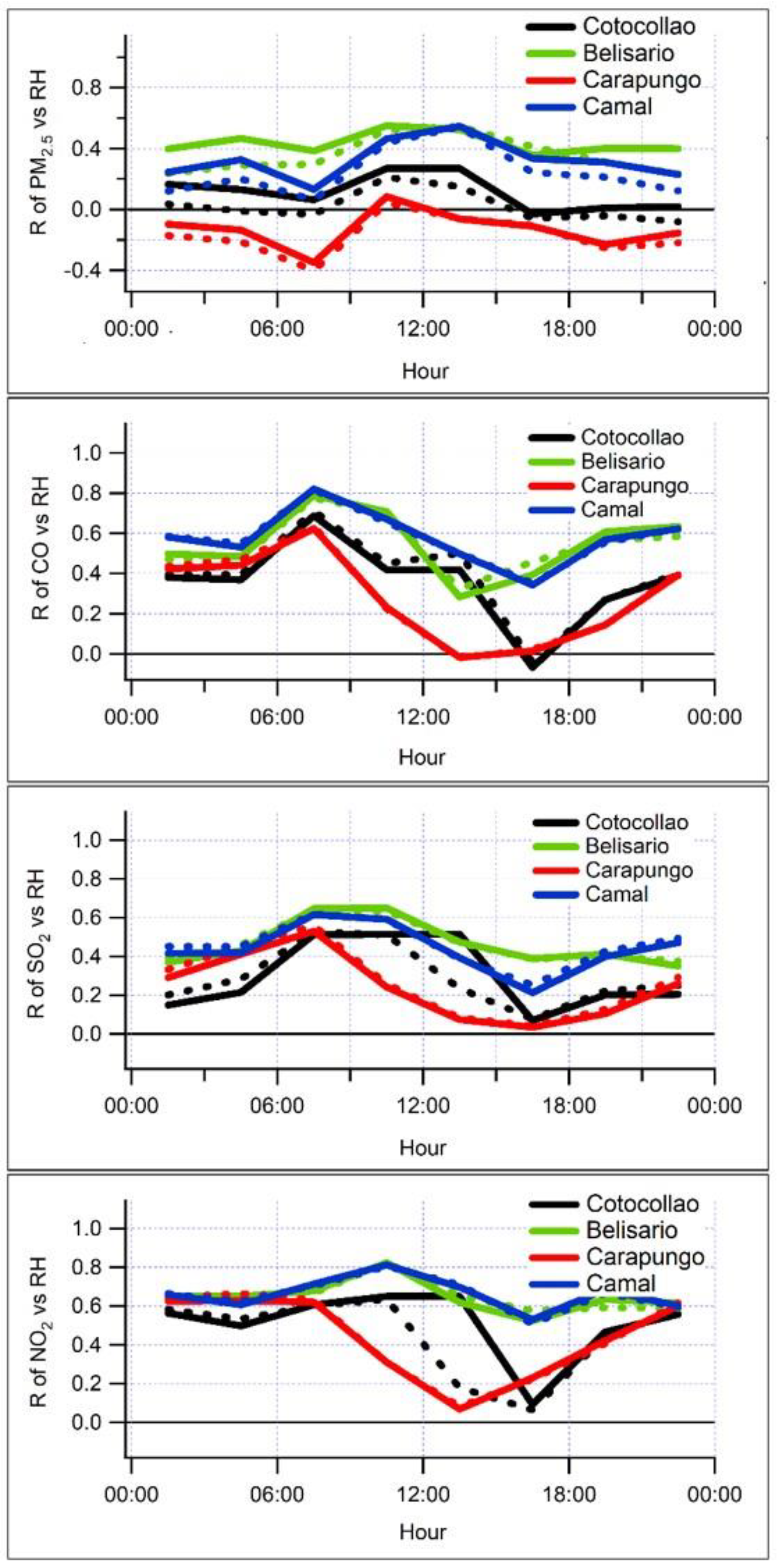
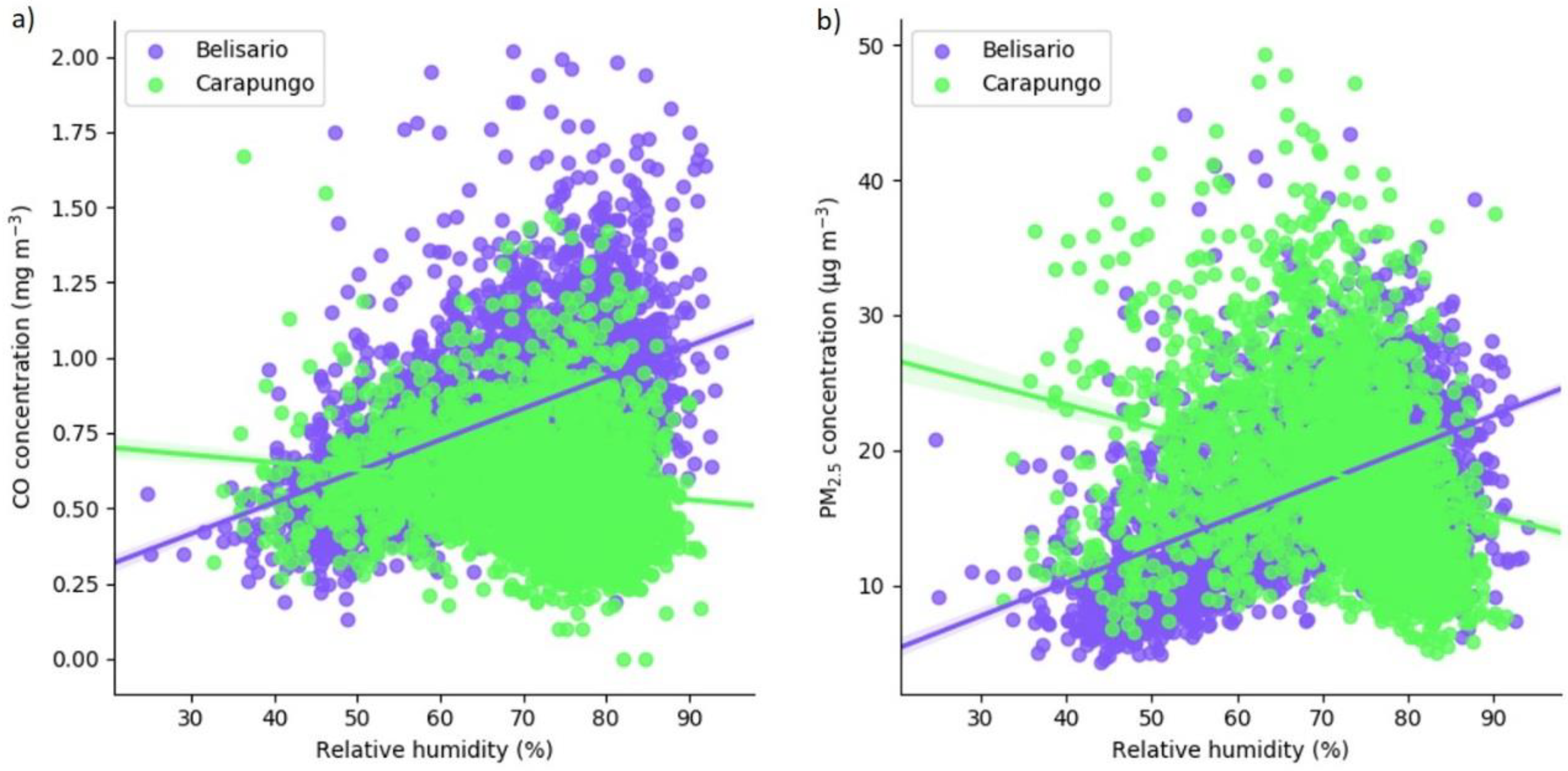
Significant positive RH vs. PM_2.5, CO, SO₂ and NO₂ correlations were found in the central Belisario area (Table A1 and Table A2, Appendix A). An additional 3-h average analysis also showed a stronger positive correlation during the rush hours for all the sites (except PM_2.5 in Carapungo) (Figure A1, Appendix B). The two sites showing the most different correlations between RH and pollution are Belisario, a lightly residential area surrounded by a dense urban street network, and Carapungo, a highly industrial area (Figure 1). A t-test shows a strong significant interaction effect between these two sites (Belisario vs. Carapungo) for relative humidity and PM_2.5 (p = 0.000) and CO (p = 0.000) concentrations. This outcome is a statistical confirmation that, the more the RH increases, the more the PM_2.5 and CO concentrations increase in the traffic-busy Belisario site, while it is opposite in the industrial Carapungo site (Figure 2).

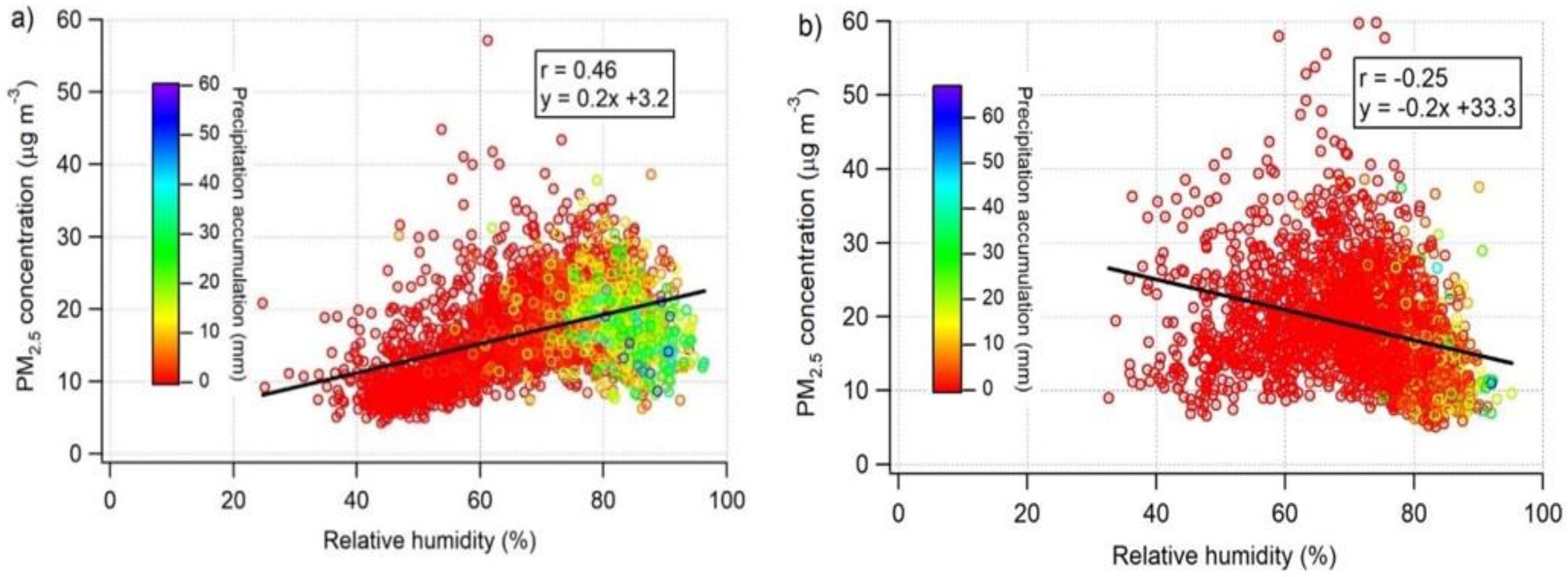
To further study the RH effect on fine particulate pollution, the average daily PM_2.5 concentrations and the daily RH data correlation analysis for the period 2007–2016 were performed (Figure 3). For the traffic-busy Belisario site, data show that, the higher the daily average RH, the higher is the PM_2.5 concentration (r = 0.46) (see Figure 3a). In addition, the same positive dependence trend was identified for the effect of absolute humidity on the PM_2.5 pollution (r = 0.46). However, the daily PM_2.5 average concentrations begin to decrease when RH reaches a certain high threshold level around 70%. Although the average daily RH varies from 40% to 95%, at high RH, it is difficult to identify a trend in the PM_2.5 concentrations. While the highly residential Cotocollao and Chillos sites had a similar positive correlation trend to the traffic-busy Belisario site, the industrial Carapungo and Camal sites had a negative correlation between RH and PM_2.5 concentrations (Figure 3b and Appendix A). This suggests that the RH effect on PM_2.5 concentrations depends on the type of the aerosol source, which is coherent with the nature of the urban areas depicted in Figure 1.

As high RH and elevation both reduce the oxygen in the intake air of internal combustion engines, this results in incomplete combustion, producing greater PM_2.5 emissions at the level of each individual vehicle. Any increase in the RH also favors nucleation of sulfuric acid during the exhaust dilution, thereby increasing the formation of PM [10,30]. This effect is of greater relevance in cities with motorized fleets that consume fuels with a high sulfur content, common in developing countries. Since the RH reduces the motor performance, it suggests that the source of pollution is (mostly) traffic based in Belisario (and Cotocollao and Chillos) and more industry based in Carapungo (and Camal). In addition, previous study has suggested that the principal source of air pollution in Carapungo seems different from the central Quito site, since it is minimally brought by the main traffic highway [12]. These differences over quite a small area are caused by the fact that the city is positioned in very complex terrain, forming microclimates with different weather conditions. Moreover, in most Latin American urban areas, there is a strong social segregation. Therefore, a different pollution correlation was found in the two poorer areas of Quito, the outskirts in the south and north, where, in addition to industrial activities, the other pollution sources might be more difficult to identify, for example charcoal cooking (in the streets), worse roads, older vehicles, poorer maintenance, etc.

3.3. Contrasted Precipitation Effect on RH Impact on PM_2.5 Concentrations

Since high RH is often a predictor of precipitation events, precipitation accumulation was added as a third component (color scale) in Figure 3. In the case of the traffic-busy Belisario site (Figure 3a), high RH with precipitation decreases PM_2.5 concentrations due to wet deposition processes such as precipitation scavenging of particles and below-cloud scavenging of gases [43]. In the case of the industrial Carapungo site, the overall influence of the rainfall on the RH and PM_2.5 correlation is negative (see Figure 3b).

We argue that the effect of the RH on PM_2.5 concentrations may be masked in data interpretation by the cleaning effect of rain events, thus making it necessary to differentiate the rainfall. 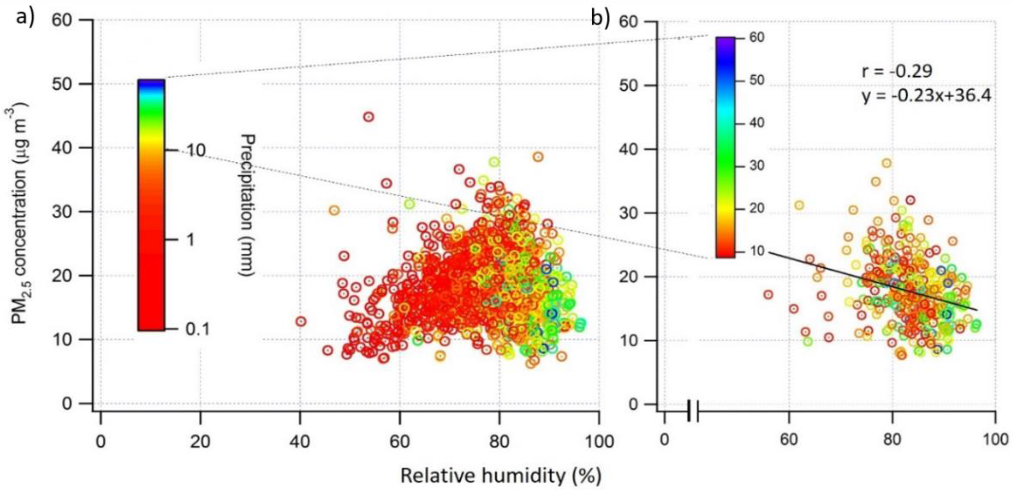Therefore, to further study the precipitation effect on RH impact on PM_2.5 pollution, we split the daily data into two separate analyses: (i) the RH and PM_2.5 correlation with daily rain accumulation; and (ii) the RH and PM_2.5 correlation without daily rain accumulation. In the traffic-busy areas of central Quito, the level of rain accumulation affects the PM_2.5 pollution (see Figure 4 for Belisario). We estimated that PM_2.5 and RH correlation coefficient changes from positive values to negative when daily precipitation accumulation is over 1 mm, confirming the findings in Zanzhou, China (elevation 1520 m.a.s.l.) [14]. The latter study indicates that, while the coarse particles (>2.5 μm) are scavenged by almost any amount of precipitation, to remove the fine and submicron aerosols they have to be exposed to a much stronger rain event. Thus, with daily rain accumulation of up to 1 mm (red markers, Figure 4a) and low RH, the daily average PM_2.5 concentrations increase with increasing RH. The correlation coefficient stabilizes from 1 mm to 8 mm of daily precipitation accumulation (at r = −0.26), and becomes more significantly negative after 9 mm, which was identified in this study as a threshold for a strong rain event. As an example, during days of light to moderate rainfall (1–8 mm), the average RH is 76% and the PM_2.5 concentrations are 18.9 µg/m³ whereas during days of stronger rain events (>9 mm), the average RH is 83% and the PM_2.5 concentrations are 17.7 µg/m³. In the case of more substantial rain accumulation, the average daily PM_2.5 concentrations decrease notably (r > −0.29) with higher RH (rainbow markers, Figure 4b), indicating a cleaning effect of precipitation. This type of analysis was not necessary for the industrial Carapungo site, as the correlation is always negative and increasing RH independently of precipitation always helps reduce the concentrations of all atmospheric criteria pollutants (Figure 3b).

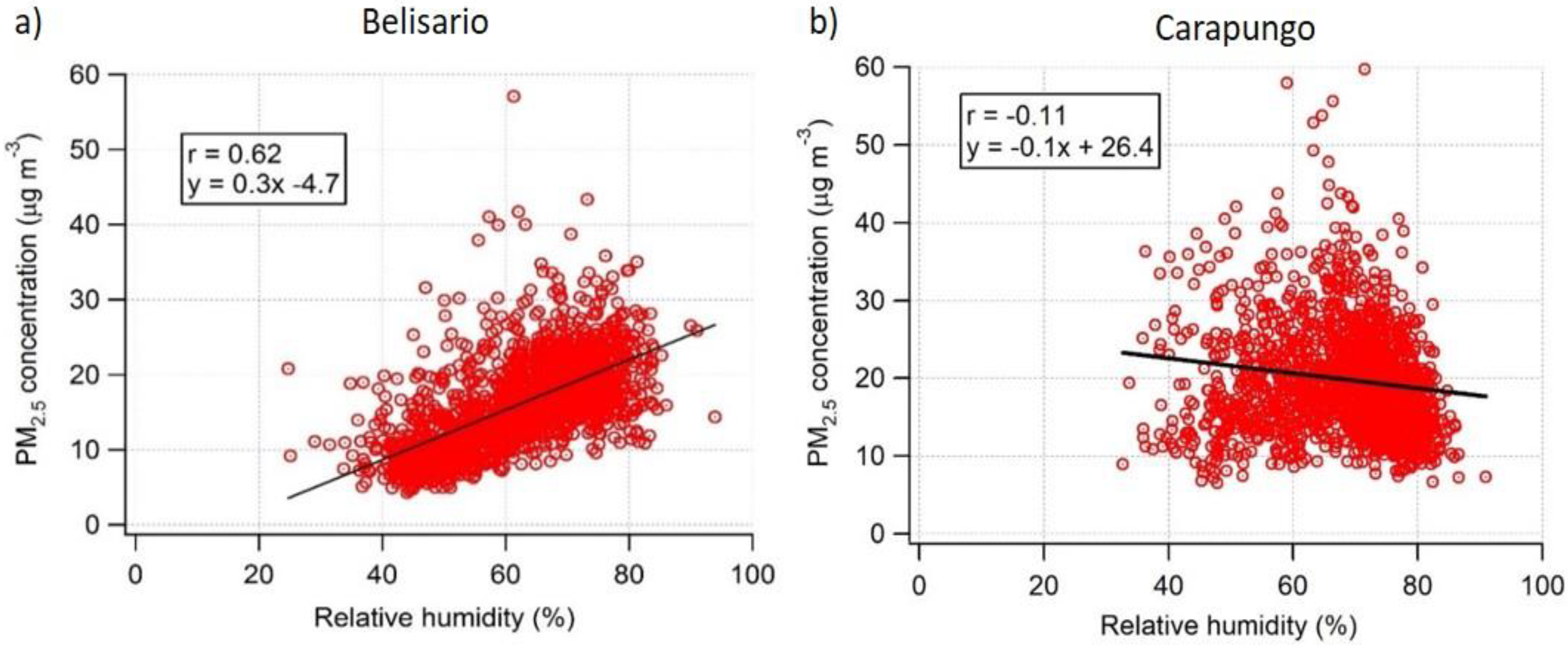
In the case of rain-free days in Belisario, the daily average RH varies from about 40% to 85% (averaging 62%) with daily average PM_2.5 concentrations varying from 8 to 22 µg/m³ (averaging 15.9 µg/m³) (Figure 5a). This analysis confirms that daily average concentrations of PM_2.5 increase (r = 0.62) with increasing average RH. The better correlation coefficient of PM_2.5 concentrations to RH on days with no rain events confirms the scavenging effect of precipitation. We can also conclude that daily average PM_2.5 concentrations above healthy limits (>25 µg/m³) are commonplace in the presence of high RH. We also highlight that the average daily PM_2.5 concentration is higher during the days with rain events, independently of the rain accumulation, if compared to the days without precipitation. This could be explained by higher relative humidity during those days, causing reduced combustion efficiency. For the industrial Carapungo site, Figure 5b shows that the increasing relative humidity even during the days of no rain events results in a negative correlation, suggesting other removal processes in the area. Carapungo is prone to night fog episodes, which might explain the PM_2.5 removal effect of high relative humidity in the absence of rain events.

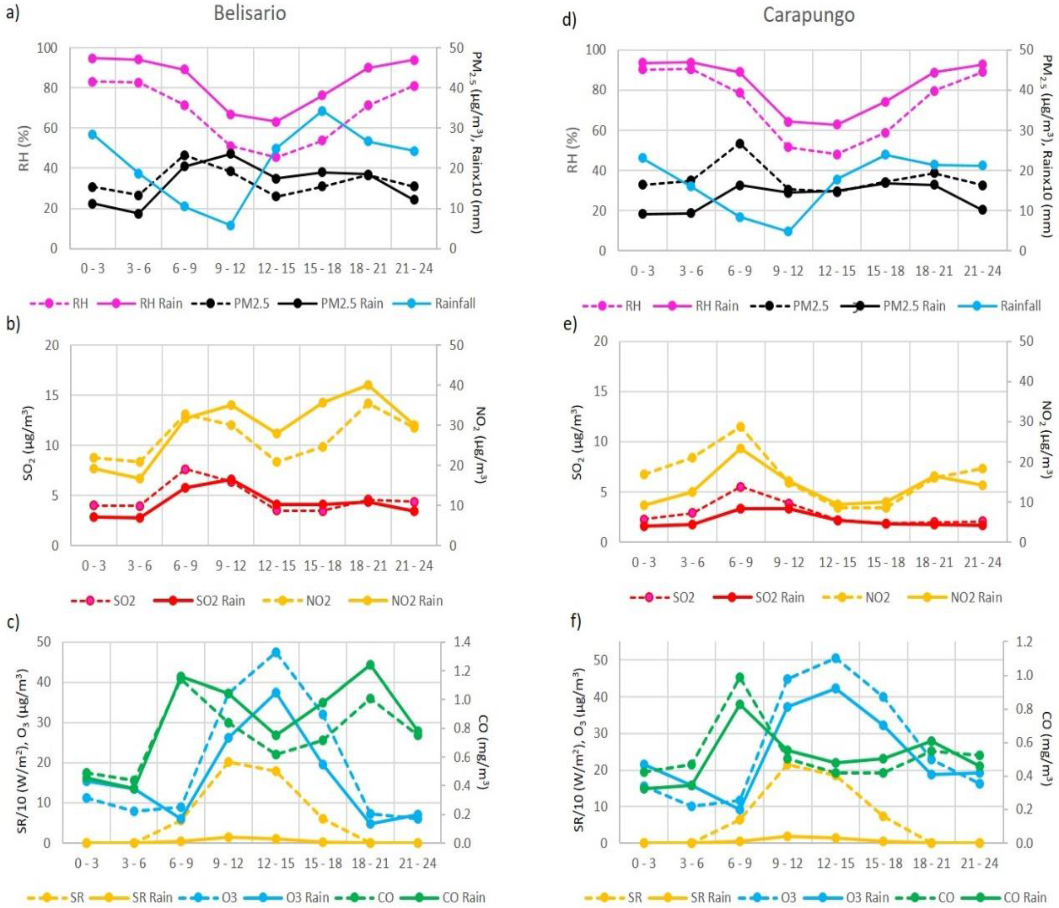
A 3-h average data analysis was performed separately for the days with rain events and no rain events. First, the data show that RH is higher during the days with rain events, and more so for the central traffic-busy Belisario site (10–20% higher) (Figure 6a). In addition, the precipitation events are common in the afternoon, and are stronger (more accumulation) at this site. The only similarity between the two contrasting sites is ozone that is present in significantly lower concentrations during the rainy days, due to the reduced photochemistry, caused by the drop in solar radiation (Figure 6c,d). The data show that, at night and early morning the PM_2.5 (Figure 6a,d), CO (Figure 6c,d), NO₂ and SO₂ (Figure 6b,e) concentrations are higher during the days with no rain if compared to the days with rain. Meanwhile, during the daytime, the fine particle and gas pollution is relatively higher if it rains that day in the traffic-busy Belisario site. In the industrial Carapungo site, the NO₂ and CO increases during the rush hours, suggesting the effect of reduced combustion efficiency. This confirms our previous findings of categorization of rain event strength, showing an increase in PM_2.5 concentrations during the minimum rain accumulation at 9:00-12:00. The latter depends on solar radiation, which is reduced during the rainy days, due to an increased cloud cover, and due to NO₂-containing products transferring to particle phase during the high RH events [44]. It can be noted that the RH variation is lower, and overall values are higher in industrial Carapungo without rain events, if compared to the traffic-busy Belisario site. The precipitation accumulation is lower in this area, suggesting other type of particle removal mechanisms, such as fog and low clouds. This high altitude region is often covered by clouds during the dark hours of the day. Finally, in both contrasting sites (and the rest of Quito), there is less diurnal variation in PM_2.5 concentrations during the days with precipitation events, or lack of rush hour traffic peak. The PM_2.5 concentrations decrease during the days with rain events, indicating the clearing effect of precipitation. In the central traffic-busy Belisario site, in addition, the morning rush hour peak shifts one hour later, which can be explained by an increase in traffic in general, traffic collapse, people being late, and increased taxi use (longer rush hour).

According to the IMPROVE formula [45,46,47,48,49,50,51,52,53], the light extinction factor of the atmosphere depends on the chemical composition of the particles, and its hygroscopic growth ability as a function of relative humidity. Thus, depending on the chemistry of the particle, it might contain more water in the events of increasing relative humidity. This would result in an increase in concentrations with increasing RH. In our study, we registered a clear increase in the particle concentrations with an increasing RH in the traffic-busy residential areas, while, in the industrial areas, we see a decreasing effect. This suggests a contrasting effect of PM and RH due to different particle chemistry. This confirms the findings of other studies in industrial and rural [11,20], and urban [15,16,17,18,19,20,24,54] areas. While we are not able to provide a chemical composition analysis of PM_2.5 due to limited resources, we see that in traffic-busy areas concentrations of PM_2.5 and combustion gases increase with increasing RH. This suggests that both come from primary motorized traffic emission. In addition, several studies state that most urban particulate pollution is generated by the motorized fleet, the emissions of which increase with the increasing RH and elevation [26,27,28,29,30,31,32,33,34,35]. In addition, the diurnal trends of PM_2.5 display a clear morning rush hour peak, which might confirm that a significant fraction of PM_2.5 is of primary origin [55,56]. 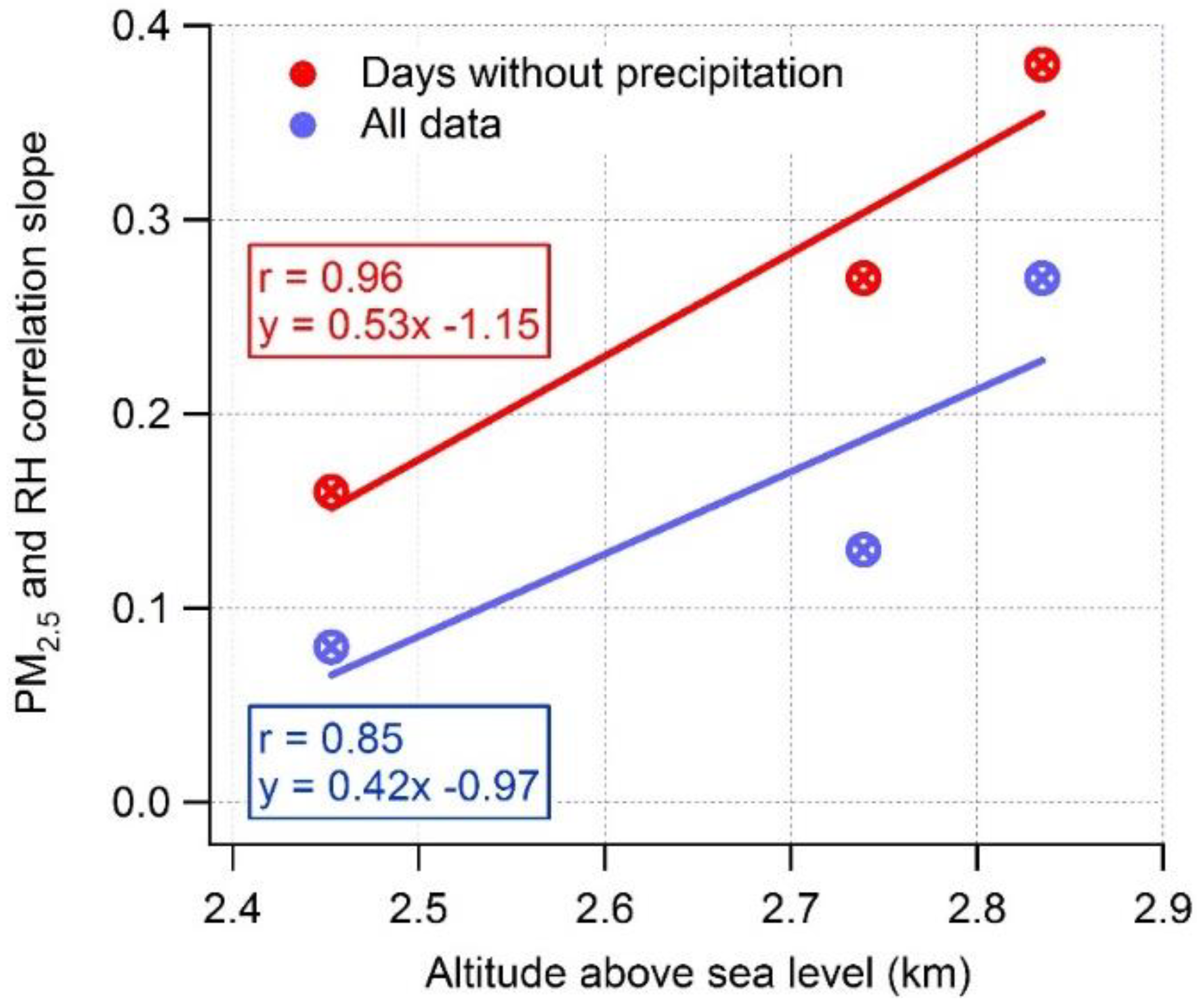The IMPROVE formula is strongly based on the secondary aerosol (ammonia and nitrate) fraction, which might suggest that it would not greatly change the variation in PM_2.5 concentrations due to water content [24,54,57]. Finally, our instruments are equipped with the heated sampling tube that removes water in the events of RH above 35%.

In addition to the effect of RH on aerosol pollution in cities at high elevations, there are several other transport-related factors that trigger higher emissions, such as road surface quality, brakes and tire wear due to more speeding and braking required where the roads are on slopes. In the case of Quito, the driving style and the conditions result in more braking and accelerating and, thus, more PM_2.5 emissions, all of which are amplified by elevation [30]. Furthermore, vehicle exhaust emissions may impact the surrounding engines’ combustion efficiency in conditions combining high elevation and RH, a fact of even greater significance in cities with multiple traffic jams.

3.4. RH Effect on PM_2.5 at Different Altitudes

For Quito, which contains several valleys and slopes at different elevations, an additional analysis was performed to investigate the elevation impact on PM_2.5 concentrations in relation to RH. We present a correlation analysis for three sites at different elevations: Chillos (elevation 2453 m.a.s.l.), Cotocollao (elevation 2739 m.a.s.l.) and Belisario (elevation 2845 m.a.s.l.) (Figure 7). We found a positive correlation between the elevation and PM_2.5 and RH regression slopes. Figure 7 shows the differentiated analysis of all the data (blue markers) and the data without rain events (red markers). We can see that the PM_2.5 and RH regression slope increases—the RH humidity effect is stronger on PM_2.5 concentrations—as the site elevation increases. The relationship between the PM_2.5 and RH correlation slope and altitude is better (r = 0.96 vs. r = 0.85) for the days with no rain events. In addition, we can see that PM_2.5 and RH regression slopes are larger (40–107%) and positive when rain events are removed from the data (red markers, Figure 7).

3.5. Models

The long-term median PM_2.5 concentration of 17.0 µg/m³ for Quito was used to study the dependence of PM_2.5 concentrations on daily precipitation and the RH (Figure 8). This classification boundary indicates whether the PM_2.5 concentrations are above or below the median value, which is preferred to the average, because it allows us to get fully balanced classes (same number of instances or observations in each class). In machine learning, if the classes are not balanced, there is a risk that the algorithm classifies on the majority class. In other words, by using the median, we assure that the classification baseline is 50% (random choice between the two possible classes). Thus, the objective is to produce a model that provides an accurate classification significantly better than 50%. Moreover, the long-term median (17.0 µg/m³) and the average (17.1 µg/m³) values are very close to each other, therefore the classification boundary in this case will result in similar boundary even if the average value was used. A logistic regression was used to minimize a cost function J(θ) such as:

$$J(\theta )=\frac{1}{m} {\displaystyle \sum }_{i=1}^m[-y^{(i)}log\left(h_{\theta }(x^{(i)})\right)-(1-y^{(i)} log(1-h_{\theta }(x^{(i)}))]$$

(1)

where m is the number of observations, y is the actual value and the hypothesis (or prediction) h_θ(x) is given by the sigmoid model as follows:

$$h_{\theta }(x)=g({\theta }^{T}x)$$

(2)

where the sigmoid function g is defined as:

$$g(z)=\frac{1}{1+e^{-z}}$$

(3)

A batch gradient descent algorithm was used to perform this minimization, in which each iteration executes the following update:

$$\frac{\partial J(\theta )}{\partial {\theta }_j}= \frac{1}{m}{\displaystyle \sum }_{i=1}^m(h_{\theta }(x^{(i)})-y^{(i)})x_j^{(i)}$$

(4)

With each step of gradient descent, the parameter θ_j comes closer to the optimal values that achieve the lowest cost J(θ). The θ_j that provides the lowest J(θ) represents the slope of the logistic regression, which best separates the two classes of PM_2.5 concentrations. Equations (5) and (6) represent the boundary, obtained using the logistic regression method, for Belisario and Carapungo, respectively. The positive value of the slope for Belisario (slope = 1.132) and the negative value of the slope for Carapungo (slope = −0.572) were calculated:

Daily precipitation accumulation = 1.132 × Daily relative humidity − 76.029

(5)

Daily precipitation accumulation = −0.572 × Daily relative humidity + 44.25

(6)

The accuracy of this classification is 69% for Belisario and 65% for Carapungo. These values are calculated through the equation as follows:

$$Accuracy= \frac{TP+TN}{TP+TN+FP+FN}$$

(7)

where TP are the true positives (>17.0 µg/m³) and TN are the true negatives (≤17.0 µg/m³). These variables are the correctly classified instances. The wrongly classified instances FP and FN are false positives and false negatives, respectively. The confusion matrix in

Table 2. Confusion matrix of the PM_2.5 classification through a logistic regression algorithm for Belisario. It is to note that the majority of instances were classified as true positive (TP) and true negative (TN), which is expected from an appropriate model.

		Classified as
		≤17 µg/m3	>17 µg/m3
Real data	≤17 µg/m3	TN = 264	FP = 155
	>17 µg/m3	FN = 104	TP = 303

and

Table 3. Confusion matrix of the PM_2.5 classification through a logistic regression algorithm for Carapungo. It is to note that the majority of instances were classified as true positive (TP) and true negative (TN), which is the expected from an appropriate model.

		Classified as
		≤17 µg/m3	>17 µg/m3
Real data	≤17 µg/m3	TN = 225	FP = 149
	>17 µg/m3	FN = 121	TP = 264

represent the way the logistic regression model classifies the data for Belisario and Carapungo, respectively. A t-test showed that the classification accuracy for both models is significantly different from the baseline (p < 0.05).

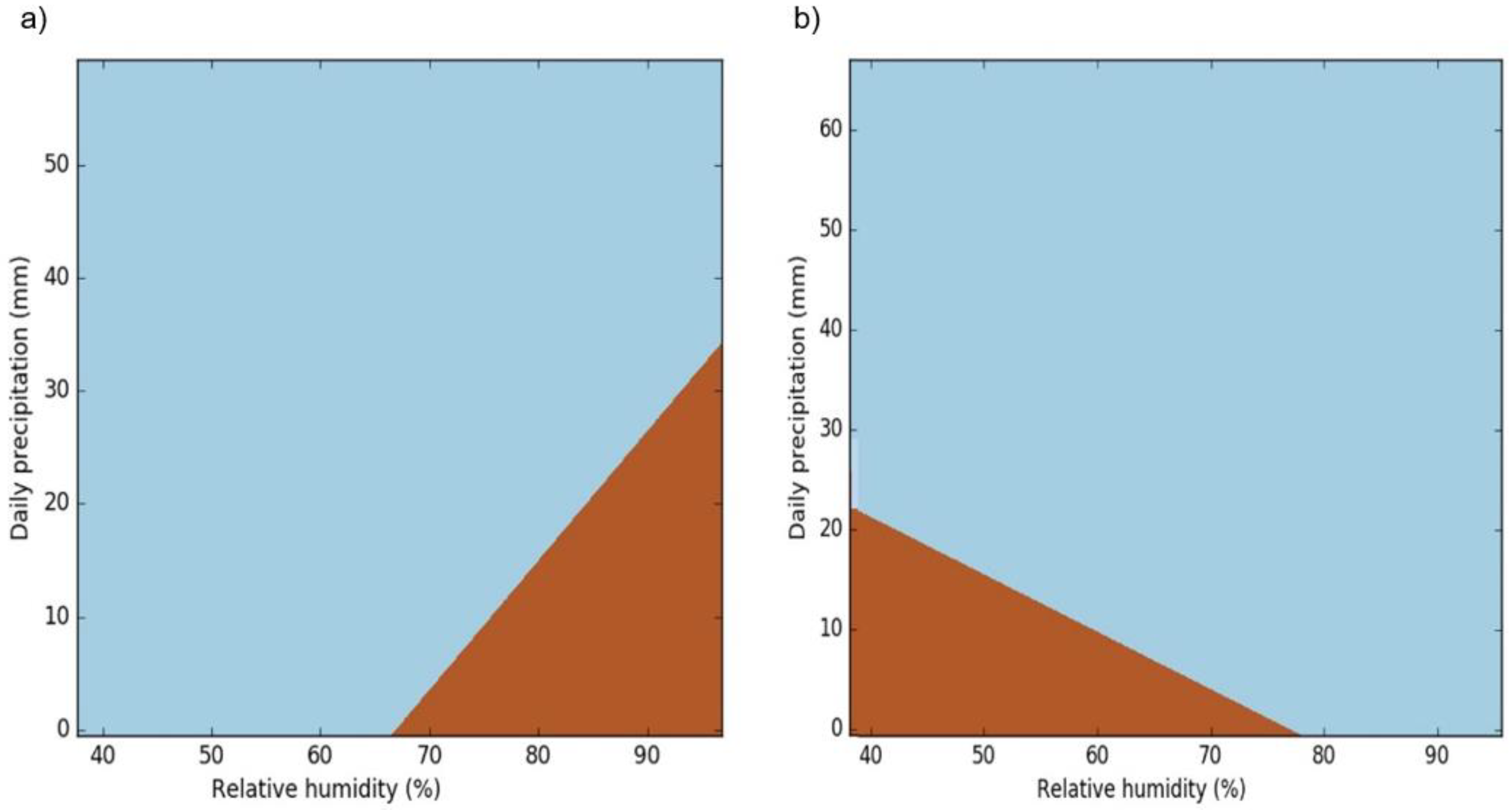
These models showed that, while, in the traffic-busy Belisario region, stronger precipitation events are necessary to reduce the PM_2.5 pollution when the RH increases, in the industrial Carapungo site, the higher the RH the lower is the pollution independently of the presence of rain. In addition, in all sites of Quito, except Carapungo, rain has an overall positive effect on the gaseous pollution, while, in most of the sites (Belisario and Chillos insignificant effect), it reduces the PM_2.5 concentrations.

In the traffic-busy Belisario, the daily average PM_2.5 concentrations were usually below 17.0 µg/m³ with RH under 67% (the blue area, Figure 8a), as can also be confirmed in Figure 3a. If the RH is over this threshold (the brown area), there must be rain to reduce the PM_2.5 concentrations to less than the median. Equation (5) identifies precisely the minimum daily precipitation accumulation required to keep PM_2.5 under 17.0 µg/m³ in relation to the RH. In the industrial Carapungo site, the effect was the opposite (Figure 3b and Figure 8b). In this industrial zone the level of rain accumulation had little effect and pollution got smaller with an increasing RH (see Equation (6) for the mathematical boundary between PM_2.5 > 17.0 µg/m³ vs. <17.0 µg/m³). Interestingly, similar results were achieved for the analysis of other chemical pollutants such as CO. This difference in the process of pollution removal between the traffic-busy Belisario and the industrial Carapungo sites suggests a distinct nature of pollution source in each site.

4. Conclusions

To the best of our knowledge, this work is the first attempt at studying the long-term impact of RH on PM_2.5 concentrations at an urban scale in a high elevation city considering the role of precipitation. There is a lack of urban pollution research at high elevations in general, while low elevation urban studies focusing on the effect of RH on pollution do not factor the precipitation component into the RH effect on the PM_2.5 concentrations. Therefore, depending on the local precipitation trends and the pollution sources, the studies may conclude a positive or a negative effect of RH on PM_2.5 concentrations.

A positive correlation between the PM_2.5 concentrations (and CO, NO₂ and SO₂) and the RH was observed in the case of residential areas with high traffic densities, while the more industrial areas showed the opposite effect. This points to the two contrasting types of sites with different PM_2.5 sources, as confirmed by interaction analysis. However, given the global trend of motorization, a positive RH effect on the PM_2.5 concentrations should be foreseen in any city but may be masked by the precipitation effect.

In the traffic-heavy area, the strong rain events played a major role in removing the fine particulate pollution. This suggests that, with future motorization and changes in climate, we may witness unpredictable mutations in urban pollution patterns. In the more industrial sites, the overall reduction of PM_2.5 concentrations was correlated with high RH regardless of the strength of the rain event. An additional analysis using a machine learning algorithm (logistic regression) allowed us to model the threshold of 17 µg/m³ for two opposite sites between high and low concentration of PM_2.5 from RH and precipitation values. These models clearly demonstrate an opposite pattern regarding the effect of the RH and precipitation on the levels of different sources of air pollution.

We see that during morning rush hours the precipitation increases the PM_2.5, CO, NO₂ and SO₂ pollution in the traffic busy areas due to two possible reasons: worsening traffic and the reduction of combustion efficiency. This means that, during the active traffic hours, the cleaning effect of the rain is not strong enough (common rain events in late afternoon), and only in the cases of strong rain events (>9 mm) is its cleaning effect notable. During the hours of low traffic, the rain effect is always notable.

Interestingly, in the traffic zones, the lowest average PM_2.5 concentrations were observed in the absence of rain, even though these PM_2.5 concentrations had the best positive correlation with the RH. This indicates that, regardless of the cleaning effect of the rain event, the PM_2.5 concentrations before and after the rain event are elevated in relation to the greatly increased RH and may thus constitute a health concern. It would be worthwhile to study the transport apportionment to PM_2.5 as evaluated during high RH events since, even in the case of lesser motorized cities, the fraction of transport-related emissions may increase during high RH episodes. Finally, this effect becomes stronger with increasing altitude.

This study concludes that RH plays a major role in producing elevated PM_2.5 concentrations in traffic congested urban areas. Therefore, the findings of this study are of greater relevance to tropical, subtropical, coastal and high elevation cities, because of reduced combustion efficiency. They should greatly apply to developing countries due to the higher sulfur content of the fuels, suggesting a serious need for investing in improving fuel quality. Based on the results of this study, it is recommended that rainfall be factored in as a third component when analyzing the effect of RH on PM_2.5 pollution, especially in cities at higher elevations, since the effect of rain events does not always result in lower average PM_2.5 concentrations, especially if the rain event is not particularly strong.

References

1. Birkmann, J. Boost resilience of small and mid-sized cities. Nature 2016, 537. [Google Scholar] [CrossRef] [PubMed]
2. WHO—Ambient (Outdoor) Air Pollution in Cities Database, 2016. Available online: http://www.who.int/phe/health_topics/outdoorair/databases/cities/en/ (accessed on 15 June 2018).
3. Gladstein Neandross & Associates. Dumping Dirty Diesels in Latin America: Reducing Black Carbon and Air Pollution from Diesel Engines in Latin American Countries; Natural Resources Defense Council: New York, NY, USA, 2014. [Google Scholar]
4. Zalakeviciute, R.; Rybarczyk, Y.; López-Villada, J.; Diaz Suarez, M.V. Quantifying decade-long effects of fuel and traffic regulations on urban ambient PM2.5 pollution in a mid-size South American city. Atmos. Pollut. Res. 2017. [Google Scholar] [CrossRef]
5. Karagulian, F.; Belis, C.A.; Dora, C.F.C.; Prüss-Ustün, A.M.; Bonjour, S.; Adair-Rohani, H.; Amann, M. Contributions to cities’ ambient particulate matter (PM): A systematic review of local sourcecontributions at global level. Atmos. Environ. 2015, 120, 475–483. [Google Scholar] [CrossRef]
6. Singh, K.P.; Gupta, S.; Rai, P. Identifying pollution sources and predicting urban air quality using ensemble learning methods. Atmos. Environ. 2013, 80, 426–437. [Google Scholar] [CrossRef]
7. Schauer, J.J.; Christensen, C.G.; Kittelson, D.B.; Johnson, J.P.; Watts, W.F. Impact of Ambient Temperatures and Driving Conditions on the Chemical Composition of Particulate Matter Emissions from Non-Smoking Gasoline-Powered Motor Vehicles. Aerosol Sci. Technol. 2008, 42, 210–223. [Google Scholar] [CrossRef] [Green Version]
8. Rönkkö, T.; Virtanen, A.; Vaaraslahti, K.; Keskinen, J.; Pirjola, L.; Lappi, M. Effect of dilution conditions and driving parameters on nucleation mode particles in diesel exhaust: Laboratory and on-road study. Atmos. Environ. 2006, 40, 2893–2901. [Google Scholar] [CrossRef]
9. Jamriska, M.; Morawska, L.; Mergersen, K. The effect of temperature and humidity on size segregated traffic exhaust particle emissions. Atmos. Environ. 2008, 42, 2369–2382. [Google Scholar] [CrossRef] [Green Version]
10. Morawska, L.; Ristovski, Z.; Jayaratne, E.R.; Keogh, D.U.; Ling, X. Ambient nano and ultrafine particles from motor vehicle emissions: Characteristics, ambient processing and implications on human exposure. Atmos. Environ. 2008, 42, 8113–8138. [Google Scholar] [CrossRef] [Green Version]
11. Li, Y.; Chen, Q.; Zhao, H.; Wang, L.; Tao, R. Variations in PM10, PM2.5 and PM1.0 in an Urban Area of the Sichuan Basin and Their Relation to Meteorological Factors. Atmosphere 2015, 6, 150–163. [Google Scholar] [CrossRef]
12. Rybarczyk, Y.; Zalakeviciute, R. Machine learning approach to forecasting urban pollution: A case study of Quito, Ecuador. In IEEE ETCM; IEEE: Guayaquil, Ecuador, 2016. [Google Scholar]
13. Kleine Deters, J.; Zalakeviciute, R.; Gonzalez, M.; Rybarczyk, Y. Modeling PM2.5 Urban Pollution Using Machine Learning and Selected Meteorological Parameters. J. Electr. Comput. Eng. 2017, 2017, 1–14. [Google Scholar] [CrossRef]
14. Feng, X.; Wang, S. Influence of different weather events on concentrations of particulate matter with different sizes in Lanzhou, China. J. Environ. Sci. 2012, 24, 665–674. [Google Scholar] [CrossRef]
15. Molina, L.T.; Madronich, S.; Gaffney, J.S.; Apel, E.; De Foy, B.; Fast, J.; Ferrare, R.; Herndon, S.; Jimenez, J.L.; Lamb, B.; et al. An overview of the MILAGRO 2006 Campaign: Mexico City emissions and their transport and transformation. Atmos. Chem. Phys. 2010, 10, 8697–8760. [Google Scholar] [CrossRef] [Green Version]
16. Wang, J.; Ogawa, S. Effects of Meteorological Conditions on PM2.5 Concentrations in Nagasaki, Japan. Int. J. Environ. Res. Public Health 2015, 12, 9089–10100. [Google Scholar] [CrossRef] [PubMed]
17. Pateraki, S.; Asimakopoulos, D.N.; Flocas, H.A.; Maggos, T.; Vasilakos, C. The role of meteorology on different sized aerosol fractions (PM10, PM2.5, PM2.5–10). Sci. Total Environ. 2012, 419, 124–135. [Google Scholar] [CrossRef] [PubMed]
18. Zhang, F.; Cheng, H.; Wang, Z.; Lv, X.; Zhu, Z.; Zhang, G.; Wang, X. ming Fine particles (PM2.5) at a CAWNET background site in Central China: Chemical compositions, seasonal variations and regional pollution events. Atmos. Environ. 2014, 86, 193–202. [Google Scholar] [CrossRef]
19. Ni, X.Y.; Huang, H.; Du, W.P. Relevance analysis and short-term prediction of PM2.5 concentrations in Beijing based on multi-source data. Atmos. Environ. 2017, 150, 146–161. [Google Scholar] [CrossRef]
20. Jayamurugan, R.; Kumaravel, B.; Palanivelraja, S.; Chockalingam, M.P. Influence of Temperature, Relative Humidity and Seasonal Variability on Ambient Air Quality in a Coastal Urban Area. Int. J. Atmos. Sci. 2013, 2013, 7. [Google Scholar] [CrossRef]
21. Sun, Y.; Wang, Z.; Fu, P.; Jiang, Q.; Yang, T.; Li, J.; Ge, X. The impact of relative humidity on aerosol composition and evolution processes during wintertime in Beijing, China. Atmos. Environ. 2013, 77, 927–934. [Google Scholar] [CrossRef]
22. Cheng, Y.; He, K.; Du, Z.Y.; Zheng, M.; Duan, F.K.; Ma, Y.L. Humidity plays an important role in the PM2.5 pollution in Beijing. Environ. Pollut. 2015, 197, 68–75. [Google Scholar] [CrossRef] [PubMed]
23. Lu, S.; Wang, D.; Li, X.; Wang, Z.; Gao, Y.; Peng, Z. Three-dimensional distribution of fine particulate matter concentrations and synchronous meteorological data measured by an unmanned aerial vehicle (UAV) in Yangtze River Delta, China. Atmos. Meas. Technol. 2016, 25, 1–19. [Google Scholar] [CrossRef]
24. Jia, L.; Xu, Y. Effects of relative humidity on ozone and secondary organic aerosol formation from the photooxidation of benzene and ethylbenzene. Aerosol Sci. Technol. 2014, 48. [Google Scholar] [CrossRef]
25. Qu, W.J.; Wang, J.; Zhang, X.Y.; Wang, D.; Sheng, L.F. Influence of relative humidity on aerosol composition: Impacts on light extinction and visibility impairment at two sites in coastal area of China. Atmos. Res. 2015, 153, 500–511. [Google Scholar] [CrossRef]
26. Tsunemoto, H.; Ishitani, H. The Role of Oxygen in Intake and Exhaust on NO Emission, Smoke and BMEP of a Diesel Engine with EGR System. SAE Tech. Pap. 1980. [Google Scholar] [CrossRef]
27. McCormick, R.L.; Graboski, M.S.; Newlin, A.W.; Ross, J.D. Effect of Humidity on Heavy-Duty Transient Emissions from Diesel and Natural Gas Engines at High Altitude. J. Air Waste Manag. Assoc. 1997, 47, 784–791. [Google Scholar] [CrossRef] [Green Version]
28. Rahai, H.R.; Shamloo, E.; Bonifacio, J.R. Investigation of the Effect of a Humid Air System on Diesel NOx and PM Emissions of a Small Diesel Engine. SAE Tech. Pap. 2011. [Google Scholar] [CrossRef]
29. Myung, C.L.; Park, S. Exhaust nanoparticle emissions from internal combustion engines: A review. Int. J. Automot. Technol. 2012, 13, 9–22. [Google Scholar] [CrossRef]
30. Wang, X.; Ge, Y.; Yu, L.; Feng, X. Effects of altitude on the thermal efficiency of a heavy-duty diesel engine. Energy 2013, 59, 543–548. [Google Scholar] [CrossRef]
31. He, C.; Ge, Y.; Ma, C.; Tan, J.; Liu, Z.; Wang, C.; Yu, L.; Ding, Y. Emission characteristics of a heavy-duty diesel engine at simulated high altitudes. Sci. Total Environ. 2011, 409, 3138–3143. [Google Scholar] [CrossRef] [PubMed]
32. Kittelson, D.; Abdul-khalek, I. Formation of Nanoparticles during Exhaust Dilution. In Fuels, Lubricants Engines & Emission; University of Minnesota: Minneapolis, MN, USA, 1999. [Google Scholar]
33. Kittelson, D.; Kraft, M.; Street, P.; Street, P. Particle Formation and Models in Internal Combustion Engines; University of Cambridge, Computational Modelling Group: Cambridge, UK, 2014. [Google Scholar]
34. Schäfer, K.; Elsasser, M.; Arteaga-Salas, J.M.; Gu, J.; Pitz, M.; Schnelle-Kreis, J.; Cyrys, J.; Emeis, S.; Prévôtt, A.S.H.; Zimmermann, R. Impact of meteorological conditions on airborne fine particle composition and secondary pollutant characteristics in urban area during winter-time. Meteorol. Z. 2016, 25, 267–279. [Google Scholar] [CrossRef]
35. Platt, S.M.; El Haddad, I.; Pieber, S.M.; Zardini, A.A.; Suarez-Bertoa, R.; Clairotte, M.; Daellenbach, K.R.; Huang, R.J.; Slowik, J.G.; Hellebust, S.; et al. Gasoline cars produce more carbonaceous particulate matter than modern filter-equipped diesel cars. Sci. Rep. 2017, 7, 1–9. [Google Scholar] [CrossRef] [PubMed]
36. Raysoni, A.U.; Armijos, R.X.; Weigel, M.M.; Montoya, T.; Eschanique, P.; Racines, M.; Li, W.W. Assessment of indoor and outdoor PM species at schools and residences in a high-altitude Ecuadorian urban center. Environ. Pollut. 2016, 214, 668–679. [Google Scholar] [CrossRef] [PubMed] [Green Version]
37. Cheng, Z.; Luo, L.; Wang, S.; Wang, Y.; Sharma, S.; Shimadera, H.; Wang, X.; Bressi, M.; de Miranda, R.M.; Jiang, J.; et al. Status and characteristics of ambient PM2.5 pollution in global megacities. Environ. Int. 2016, 89–90, 212–221. [Google Scholar] [CrossRef] [PubMed]
38. Vega, D.; Ocaña, L.P.R. Inventario de Emisiones Atmosféricas del Tráfico Vehicular Y Gasolineras del Distrito Metropolitano de Quito Año Base 2012; Universidad San Francisco de Quito: Quito, Ecuador, 2015. [Google Scholar]
39. Municipio del Distrito Metropolitano de Quito: Plan de Desarrollo 2012–2022; EMASEO: Quito, Ecuador, 2011.
40. Poblacion, Superficie (km2), Densidad Poblacional a Nivel Parroquial; INEC: Ecuador, Quito, 2011.
41. Huryn, S.M.; Gough, W.A. Impact of urbanization on the ozone weekday/weekend effect in Southern Ontario, Canada. Urban Clim. 2014, 8, 11–20. [Google Scholar] [CrossRef]
42. Raysoni, A.U.; Armijos, R.X.; Margaret Weigel, M.; Echanique, P.; Racines, M.; Pingitore, N.E.; Li, W.W. Evaluation of sources and patterns of elemental composition of PM2.5 at three low-income neighborhood schools and residences in Quito, Ecuador. Int. J. Environ. Res. Public Health 2017, 14, 674. [Google Scholar] [CrossRef] [PubMed]
43. Seinfeld, J.H.; Pandis, S.N. Atmospheric Chemistry and Physics, 3rd ed.; John Wiley & Sons, Inc.: Hoboken, NJ, USA, 2016; ISBN 9781118947401. [Google Scholar]
44. Yu, X.; Ma, J.; An, J.; Yuan, L.; Zhu, B.; Liu, D.; Wang, J.; Yang, Y.; Cui, H. Impacts of meteorological condition and aerosol chemical compositions on visibility impairment in Nanjing, China. J. Clean. Prod. 2016, 131, 112–120. [Google Scholar] [CrossRef]
45. Hand, J.; Malm, W.C. Review of the IMPROVE Equation for Estimating Ambient Light Extinction Coefficients; Colorado State University: Fort Collins, CO, USA, 2007. [Google Scholar]
46. Hyslop, N.P.; White, W.H. An evaluation of interagency monitoring of protected visual environments (IMPROVE) collocated precision and uncertainty estimates. Atmos. Environ. 2008, 42, 2691–2705. [Google Scholar] [CrossRef]
47. Pitchford, M.; Malm, W.; Schichtel, B.; Kumar, N.; Lowenthal, D.; Hand, J. Revised algorithm for estimating light extinction from IMPROVE particle speciation data. J. Air Waste Manag. Assoc. 2007, 57, 1326–1336. [Google Scholar] [CrossRef] [PubMed]
48. Tao, J.; Cao, J.-J.; Zhang, R.-J.; Zhu, L.; Zhang, T.; Shi, S.; Chan, C.-Y. Reconstructed light extinction coefficients using chemical compositions of PM2.5 in winter in Urban Guangzhou, China. Adv. Atmos. Sci. 2012, 29, 359–368. [Google Scholar] [CrossRef]
49. Malm, W.C.; Day, D.E.; Kreidenweis, S.M.; Collett, J.L.; Lee, T. Humidity-dependent optical properties of fine particles during the Big Bend Regional Aerosol and Visibility Observational Study. J. Geophys. Res. Atmos. 2003, 108. [Google Scholar] [CrossRef] [Green Version]
50. Lowenthal, D.H.; Kumar, N. Evaluation of the IMPROVE Equation for estimating aerosol light extinction. J. Air Waste Manag. Assoc. 2016, 66, 726–737. [Google Scholar] [CrossRef] [PubMed] [Green Version]
51. Hwang, I.J.; Hopke, P.K. Estimation of source apportionment and potential source locations of PM2.5 at a west coastal IMPROVE site. Atmos. Environ. 2007, 41, 506–518. [Google Scholar] [CrossRef]
52. Ryan, P.A. Precipitation in light extinction reconstruction. J. Air Waste Manag. Assoc. 2005, 55, 1014–1018. [Google Scholar] [CrossRef] [PubMed]
53. Ryan, P.A.; Lowenthal, D.; Kumar, N. Improved light extinction reconstruction in interagency monitoring of protected visual environments. J. Air Waste Manag. Assoc. 2005, 55, 1751–1759. [Google Scholar] [CrossRef] [PubMed]
54. Wang, X.; Wang, W.; Yang, L.; Gao, X.; Nie, W.; Yu, Y.; Xu, P.; Zhou, Y.; Wang, Z. The secondary formation of inorganic aerosols in the droplet mode through heterogeneous aqueous reactions under haze conditions. Atmos. Environ. 2012, 63, 68–76. [Google Scholar] [CrossRef]
55. Zalakeviciute, R.; Alexander, M.L.; Allwine, E.; Jimenez, J.L.; Jobson, B.T.; Molina, L.T.; Nemitz, E.; Pressley, S.N.; Vanreken, T.M.; Ulbrich, I.M.; et al. Chemically-resolved aerosol eddy covariance flux measurements in urban Mexico City during MILAGRO 2006. Atmos. Chem. Phys. 2012, 12, 7809–7823. [Google Scholar] [CrossRef] [Green Version]
56. Salcedo, D.; Onasch, T.B.; Dzepina, K.; Canagaratna, M.R.; Zhang, Q.; Huffmann, J.A.; DeCarlo, P.F.; Jayne, J.T.; Mortimer, P.; Worsnop, D.R.; et al. Characterization of ambient aerosols in Mexico City during the MCMA-2003 campaign with Aerosol Mass Spectrometry: Results from the CENICA Supersite. Atmos. Chem. Phys. 2006, 6, 925–946. [Google Scholar] [CrossRef]
57. Gordon, C.A.; Ye, J.; Chan, A.W.H. Secondary Organic Aerosol Formation Enhanced by Organic Seeds of Similar Polarity at Atmospherically Relative Humidity. STEM Fellowsh. J. 2016, 1, 6–10. [Google Scholar] [CrossRef]
Figure 1. Locations of air quality measurement sites (blue dots) in the metropolitan area of Quito, Ecuador, in relation to the industrial parks (pink areas), thermoelectric power stations (red points) and mining areas (yellow areas). The white color lines represent the main transport routes.
Sustainability 10 02064 g001
Figure 2. Interaction effect between RH and site (Belisario vs. Carapungo) regarding: CO concentration (a); and PM2.5 (b) concentration (studied period: 2007–2016).
Sustainability 10 02064 g002
Figure 3. Correlation analysis of average daily PM2.5 concentrations and the average daily RH over the period 2007–2016 in the central traffic-busy Belisario site (a); and in the northern industrial Carapungo sites with precipitation accumulation considered (b). The color scale of the correlation markers shows daily precipitation accumulation.
Sustainability 10 02064 g003
Figure 4. Belisario correlation analysis of PM2.5 concentrations and RH for the period 2007–2016: during days with rain events: all rain events (a); and only rain events of total daily cumulative rainfall of over 9 mm (strong rain events) (b).
Sustainability 10 02064 g004
Figure 5. Correlation analysis of the average daily PM2.5 concentrations and the average daily RH during 2007–2016: for days with no rain events in the traffic-busy Belisario (a); and the industrial Carapungo (b) sites.
Sustainability 10 02064 g005
Figure 6. Three-hour evolution of the average relative humidity (RH), rainfall, PM2.5 (a,d), and pollutant gases concentrations and solar radiation (SR) (b,c,e,f) during the days with no rain events (dotted lines) and the days with precipitation (solid lines) for the central traffic-busy Belisario (ac) and the industrial Carapungo (df) sites.
Sustainability 10 02064 g006
Figure 7. Correlation analysis of altitude and PM2.5 and RH regression slopes at three different areas of Quito: Chillos (elevation 2453 m.a.s.l.), Cotocollao (2739 m.a.s.l.), and Belisario (2845 m.a.s.l). Blue markers show the correlation analysis of all the data, and red markers show only the data of days without rain. The data presented for two years: 2014–2016.
Sustainability 10 02064 g007
Figure 8. Logistic regression models of the PM2.5 concentrations built from the average daily RH and precipitation features over the period 2007–2016: in the central traffic-busy Belisario (a); and in the northern industrial Carapungo (b). The blue region indicates the days when PM2.5 concentrations are below 17.0 µg/m3 and the brown region when the PM2.5 concentrations are above 17.0 µg/m3.
Sustainability 10 02064 g008