A Method for Monitoring Iron and Steel Factory Economic Activity Based on Satellites

Abstract

The Chinese government has promulgated a de-capacity policy for economic growth and environmental sustainability, especially for the iron and steel industry. With these policies, this study aimed to monitor the economic activities and evaluate the production conditions of an iron and steel factory based on satellites via Landsat-8 Thermal Infrared Sensor (TIRS) data and high-resolution images from January 2013 to October 2017, and propel next economic adjustment and environmental protection. Our methods included the construction of a heat island intensity index for an iron and steel factory (ISHII), a heat island radio index for an iron and steel factory (ISHRI) and a dense classifying approach to monitor the spatiotemporal changes of the internal heat field of an iron and steel factory. Additionally, we used GF-2 and Google Earth images to identify the main production area, detect facility changes to a factory that alters its heat field and verify the accuracy of thermal analysis in a specific time span. Finally, these methods were used together to evaluate economic activity. Based on five iron and steel factories in the Beijing-Tianjin-Hebei region, when the ISHII curve is higher than the seasonal changes in a time series, production is normal; otherwise, there is a shut-down or cut-back. In the spatial pattern analyses, the ISHRI is large in normal production and decreases when cut-back or shut-down occurs. The density classifying images and high-resolution images give powerful evidence to the above-mentioned results. Finally, three types of economic activities of normal production, shut-down or cut-back were monitored for these samples. The study provides a new perspective and method for monitoring the economic activity of an iron and steel factory and provides supports for sustainable development in China.

1. Introduction

For years, the iron and steel industry as a pillar industry in China has been challenged by economic sustainability and has suffered from environmental policy pressure. The relationship between economic growth, natural limits, and environmental sustainability has always been a focus of research [1], and the iron and steel production process, as the largest consumer of electricity and fossil fuels [2], is closely related to mineral resource utilization, water consumption, greenhouse gas emission [3], land use and so on. In 2015, the Chinese government issued supply-side reform and a de-capacity policy for the iron and steel industry [4], especially focusing on the Beijing-Tianjin-Hebei (BTH) region where numerous iron and steel factories are concentrated [5]. Therefore, it is worthwhile to accurately monitor the economic activity of an iron and steel factory for sustainable development of the entire industry and the environment.

To date, as a special studied object, the complexity and large number of iron and steel factories have limited our ability to obtain relatively accurate information to evaluate temporal and spatial changes via conventional methods, such as manually monitoring and random checking [6] at high cost. Generally, with the advantages of speed and ease of use, spatiotemporal monitoring approaches based on satellite data have often been used for Earth observation [7], from global changes [8] to urban extension [9], but they are also gradually being applied to studying the economic environment and the specific activities of economic industries [10,11]. Some scholars use night-time light data to map regional economic activity [12,13] or evaluate economic conditions after war [14]. A company named Spaceknow Inc. released a new version of the Chinese satellite manufacturing index (SMI), which may be used to observe and explain the Chinese economy by comprising industry base images all over China [15]. More progress has been made based on satellites in economic activity on large spatial scales, but there has been no study on an individual economic object. Therefore, remote sensing approaches are introduced here to study the economic activity of an iron and steel factory for the first time.

An iron and steel factory includes sophisticated processing technology and special situations [16]. Several production sectors such as sintering emit a large amount of heat to the outside environment because they connect closely with fire [17]. The land surface temperature (LST) in the production area is higher than that in nonproduction areas, which leads to specific thermal anomalies near these production facilities [17,18]. The LST data can be obtained from ground meteorological sites [19] and retrieved using thermal infrared sensor (TIRS) bands [20]. With the increasing number of satellites and the development of geospatial information technology, many studies have widely adopted LST data from TIRS, such as AVHRR data from NOAA [21], MODIS data from the Terra/Aqua satellites [22], and TM/ETM+/TIRS data from the Landsat-5–8 satellites [23,24]. Based on LST data, studies have been conducted on geothermal exploration [25], pre-earthquake monitoring [26], surface urban heat islands [27], and identification of manufacturing industry [11]. Liu [17] found that the unusually high temperatures from industrial heat sources can be tracked by remote sensing satellite, which collects consistent and extensive data day and night. In general, numerous factors can lead to LST variations for a certain region, such as the air temperature, population density, industrial emissions and surface coverage [28,29,30]. LST variations in an iron and steel factory are primarily caused by seasonal variations, production heat emissions, and land use. Therefore, heat field analysis based on satellites may be the most effective way to monitor the dynamics of these thermal anomalies. In addition, previous studies show that change detection based on high-resolution imagery [31] from Wordview, Spot, Quikbird, Google Earth, GF-1, GF-2 [32] or other sensors is an effective method for obtaining surface change information [33].

Consequently, this study tried to provide an approach based on satellite data for monitoring economic activity of an iron and steel factory by measuring internal variations and evaluating economic conditions. For the local analysis, Landsat 8 TIRS data were chosen with a relatively high spatial resolution that greatly benefits LST inversion detection, and high-resolution images of GF-2 and Google Earth images were chosen. Based on the abovementioned remote sensing data, a systemic method and a new perspective were provided to monitor the economic activity of an iron and steel factory. Figure 1 shows the flow of this study. LST data were used to analyze the internal heat field by building the heat island intensity index of an iron and steel factory (ISHII) and the heat island ratio index of an iron and steel factory (ISHRI) in a time series. The GF-2 data were used to obtain the main surface features and changes via visual interpretation. Based on the timelines of production activity events collected on the Internet, this method was verified to be effective and can recognize economic activity changes in an iron and steel factory and evaluate the development conditions to provide objective support for sustainable development in China.

2. Study Area and Data

2.1. Study Area

The study area is located in the Beijing-Tianjin-Hebei region (BTH region) of China, which is within 113°27′–119°50′ E and 36°03′–42°40′ N [34]. The BTH region, where Tangshan and Handan are the two main cities with numerous iron and steel industrial bases, is the cradle of the Chinese manufacturing industry and suffers serious environmental pollution. In addition, the de-capacity policy initially had a great effect on small- and medium-sized iron and steel factories. Therefore, in this study, the following five typical iron and steel factories were chosen from two cities: Tangshan Beishiti Steel (Group) Co., Ltd. (Beishiti, China); Tangshan Xinglong Steel Co., Ltd. (Xinglong, China); Hebei Xinjin Iron and Steel Co., Ltd. (Xinjin, China); Hebei Zongheng Steel & Iron Group Co., Ltd. (Zonghen, China); and Antai Iron & Steel Co., Ltd. (Antai, China). Sample data obtained for these factories are shown in Figure 2. These representative factories are chosen based on their size and state of production.

2.2. Data and Preprocessing

For an iron and steel factory, the experiment requires remote sensing data with high spatial resolution. Therefore, Landsat-8 TIRS data were selected to retrieve the LST data. In addition, GF-2 data and Google Earth images were used to identify the production areas and detect facility changes. Statistical data were also collected from the Internet for auxiliary judgments and results validation.

2.2.1. Landsat 8 TIRS Data

Landsat-8 TIRS data, which have a spatial resolution of 100 m and a temporal resolution of 16 days, were directly acquired from the satellite and are suitable for studying an iron and steel factory.

Table 1. Basic information of the Landsat-8.

Band Name	Band	Spatial Resolution	Temporal Resolution
OLI 1	0.43–0.45	30 m	16 days
OLI 2	0.45–0.52	30 m
OLI 3	0.53–0.60	30 m
OLI 4	0.63–0.68	30 m
OLI 5	0.85–0.89	30 m
OLI 6	1.56–1.66	30 m
OLI 7	2.10–2.30	30 m
OLI 8	0.50–0.68	15 m
OLI 9	1.36–1.39	30 m
TIRS 1	10.6–11.2	100 m
TIRS 2	11.5–12.5	100 m

details the basic information on Landsat 8. The L1G-level of the Landsat-8 TIRS images (Path/Row: 122/32,124/35) from 2013 to 2017 were downloaded from USGS [35], with a commonly Universal Transverse Mercator (UTM) coordinate system of 50 N based on the WGS84 datum. After checking the quality of all images (primarily cloud contamination or lost header files), four images per year (in January, April, July, and October) were obtained.

Before retrieving the LST data, a series of key data preprocessing steps must be performed, such as geometric correction, radiometric calibration and extraction by each factory mask. The preprocessing emphasizes radiometric calibrations as shown in Equation (1):

$${\mathrm{L}}_{\mathsf{\lambda }}={\mathrm{M}}_{\mathrm{L}}\times {\mathrm{Q}}_{\mathrm{cal}}+{\mathrm{A}}_{\mathrm{L}}$$

(1)

where M_L is the gain parameter, which can be acquired from the metadata (RADIANCE_MULT_BAND_i); A_L is the migration parameter, which can be acquired from the metadata (RADIANCE_ADD_BAND_i); i is the band; and Qcal is the DN value of the band.

For Landsat TIRS data, the radiative transfer equation [36], mono-window algorithm [37], split-window algorithm [38] and single channel algorithms [22,39] are the most widely used to retrieve LST data. Each algorithm has limitations with errors due to atmospheric effects, complicated ground surfaces, sensor noise, wavelength uncertainty, etc. [23].

In this study, the radiative transfer equation algorithm (RTM) was employed for LST retrieval. The RTM conforms to the law of conservation of energy, thus ensuring that absorptivity, reflectivity and transmissivity sum to 1. The RTM has the advantage of using one band (band 10) and high retrieval precision [36]. The main method of LST retrieval is given as follows:

$${\mathrm{L}}_{\mathsf{\lambda }}={\mathrm{B}}_{\mathrm{i}}\left({\mathrm{T}}_{\mathrm{i}}\right)=\left[{\mathsf{\epsilon }}_{\mathrm{i}}\cdot {\mathrm{B}}_{\mathrm{i}}\left({\mathrm{T}}_{\mathrm{s}}\right)+\left(1-{\mathsf{\epsilon }}_{\mathrm{i}}\right)\mathrm{L}\downarrow \right]\cdot {\mathsf{\tau }}_{\mathrm{i}}\left(\mathsf{\theta }\right)+\mathrm{L}\uparrow$$

(2)

where ${\mathrm{B}}_{\mathrm{i}}\left({\mathrm{T}}_{\mathrm{i}}\right)$ is the radiance received by TIRS channel $\mathrm{i}$ of sensors with brightness temperature Ti; ${\mathsf{\epsilon }}_{\mathrm{i}}$ is the surface emissivity for channel $\mathrm{i}$; ${\mathrm{T}}_{\mathrm{s}}$ is the land surface Temperature (k); $\mathsf{\tau }\left(\mathsf{\theta }\right)$ is the atmospheric transmittance for channel i (when the view zenith angle is $\mathsf{\theta }$, TIRS is treated as a nadir view because the view angle is no more than 7.5°); ${\mathrm{B}}_{\mathrm{i}}\left({\mathrm{T}}_{\mathrm{s}}\right)$ is the thermal radiation intensity of the blackbody indicated by the Planck function; $\mathrm{L}\uparrow$ is the upwelling path radiant luminance ($\mathsf{\omega }\cdot {\mathrm{m}}^{-2}{\mathrm{sr}}^{-1}{\mathsf{\mu }\mathrm{m}}^{-1}$); and $\mathrm{L}\downarrow$ is the downwelling path radiant luminance ($\mathsf{\omega }\cdot {\mathrm{m}}^{-2}{\mathrm{sr}}^{-1}{\mathsf{\mu }\mathrm{m}}^{-1}$).

By Planck’s law, ${\mathrm{B}}_{\mathrm{i}}\left({\mathrm{T}}_{\mathrm{s}}\right)$ can be expressed as Equation (3):

$${\mathrm{B}}_{\mathrm{i}}\left({\mathrm{T}}_{\mathrm{s}}\right)=\frac{{\mathrm{C}}_1}{{\mathsf{\lambda }}_{\mathrm{i}}^5\left[\exp \left({\mathrm{C}}_2/{\mathsf{\lambda }}_{\mathrm{i}}{\mathrm{kT}}_{\mathrm{s}}\right)\right]-1}$$

(3)

where ${\mathrm{T}}_{\mathrm{s}}$ is the LST; k is the Boltzmann constant; ${\mathsf{\lambda }}_{\mathrm{i}}$ is the effective band wavelength for band $\mathrm{i}$; and C1 and C2 represent Planck constants. Thus, the LST can be retrieved as Equation (4):

$${\mathrm{T}}_{\mathrm{s}}=\frac{{\mathrm{C}}_1}{{\mathsf{\lambda }}_{\mathrm{i}}\ln \left(\frac{{\mathrm{C}}_2}{{\mathsf{\lambda }}_{\mathrm{i}}^5\left({\mathrm{B}}_{\mathrm{i}}\left({\mathrm{T}}_{\mathrm{i}}\right)-{\mathrm{L}}_{\uparrow }-{\mathsf{\tau }}_{\mathrm{i}}\left(1-{\mathsf{\epsilon }}_{\mathrm{i}}\right){\mathrm{L}}_{\downarrow }\right)/{\mathsf{\tau }}_{\mathrm{i}}{\mathsf{\epsilon }}_{\mathrm{i}}}+1\right)}$$

(4)

Because of the difficulties encountered in obtaining real-time atmospheric profile data$,{\mathsf{\tau }}_{\mathrm{i}}\left(\mathsf{\theta }\right)$, $\mathrm{L}\uparrow$, and $\mathrm{L}\downarrow$ can be simulated by standard atmospheric profile data and acquired by importing the imaging time, central latitude and longitude, regional pressure and other related information from NASA [40]. Emissivity is an important parameter for representing the thermal radiation properties of objects in most retrieval algorithms [41,42]. A mixed pixel decomposition method reported by Qin [42] based on TM images was used in this experiment to calculate the emissivity.

According to the RTM, LST data can be retrieved. Figure 3 shows an example image for the iron and steel factory of Zongheng on 2 May 2017.

2.2.2. High-Resolution Images

With the development of remote sensing technology, sub-meter multispectral comprehensive optical remote sensing data can be obtained. GF-2 and Google Earth images were chosen to identify production areas and detect surface changes in the iron and steel factories. GF-2 data features a high spatial resolution and location accuracy, including accuracies of up to 1 m in the panchromatic band and 4 m in the spectral band; these data could be acquired starting in late 2014 [40].

Table 2. GF-2 basic information.

Band Name	Number	Band	Spatial Resolution	Temporal Resolution
PAN 1	1	0.45–0.90	1 m	5 days
MSS 2	2	0.45–0.52	4 m
	3	0.52–0.59	4 m
	4	0.63–0.69	4 m
	5	0.77–0.89	4 m

¹ Panchromatic band; ² Multi Spectral Scanner.

depicts the basic information.

Due to the influence of the sensor on external factors, the accuracy of the original image is reduced and preprocessing must be performed to improve the data quality. The preprocessing of GF-2 images includes forward correction, image registration, image fusion and atmospheric correction, as shown in Figure 4.

2.2.3. Auxiliary Data

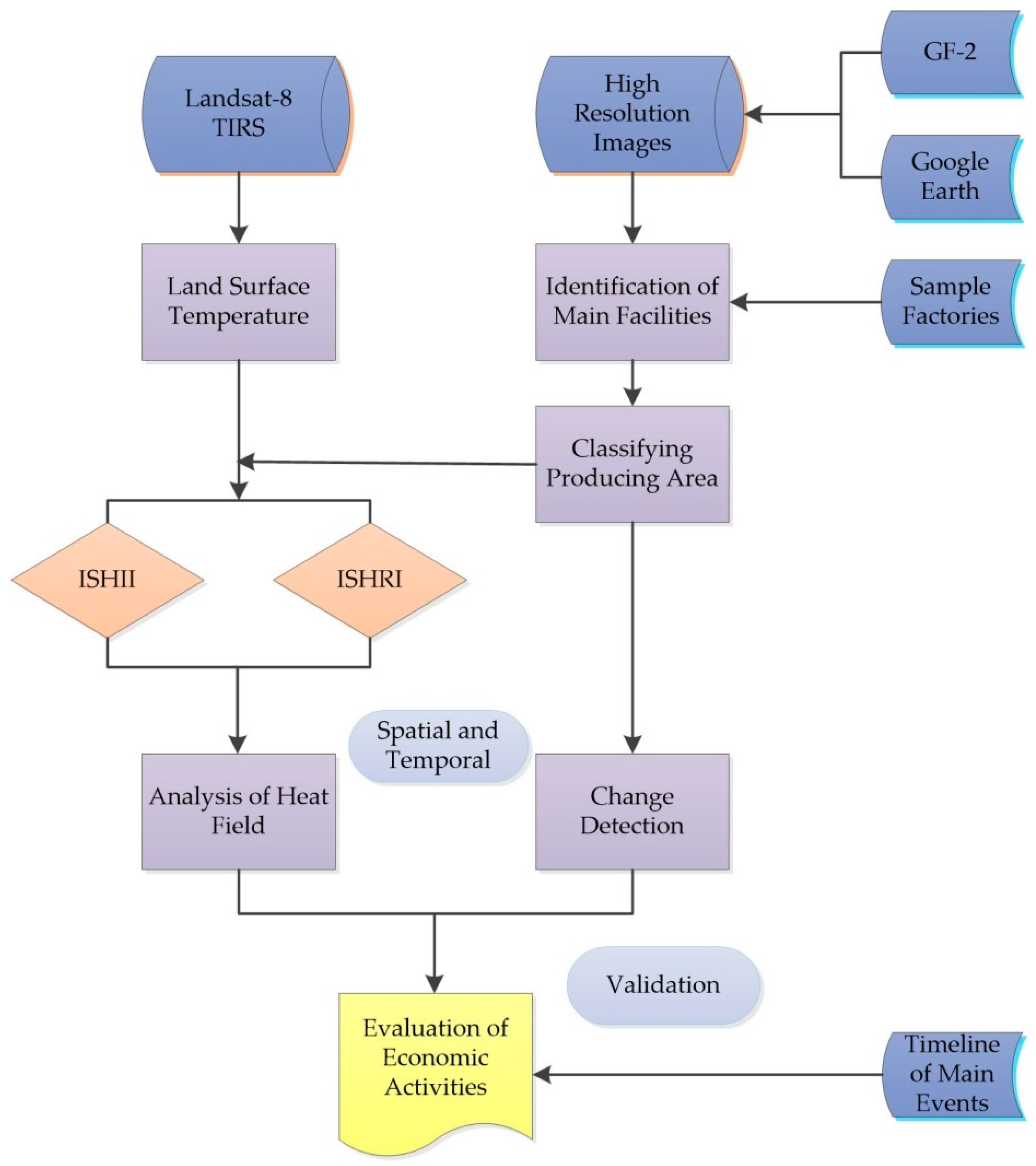
To explain the changes in the heat field, certain production events of the samples were collected on the Internet [43] from 2013 to 2017. These events pertain to when the related iron and steel factories stopped or started producing or what specific changes were made in the facilities. A timeline of these events is shown in Figure 5 and the basic information of samples in

Table 3. The basic information of sample factories from the Internet.

Name	Area	Furnace	Converter	Production	Workers
Antai	74 ha	1 × 450 m3, 1 × 1080 m3	1 × 32 t, 2 × 35 t	200 kt	-
Beishiti	38 ha	2 × 600 m3	2 × 55 t	-	3000
Xinglong	-	1 × 450 m3, 1 × 530 m3, 1 × 1080 m3	3 × 50 t	200 kt	-
Xinjin	-	2 × 1280 m3, 2 × 2080 m3, 2 × 450 m3, 1 × 600 m3, 2 × 1080 m3	2 × 40 t, 2 × 120 t	515 kt	6500
Zongheng	-	4 × 580 m3	2 × 85 t	500 kt	4000

.

3. Methodology

3.1. Identification and Change Detection Based on GF-2

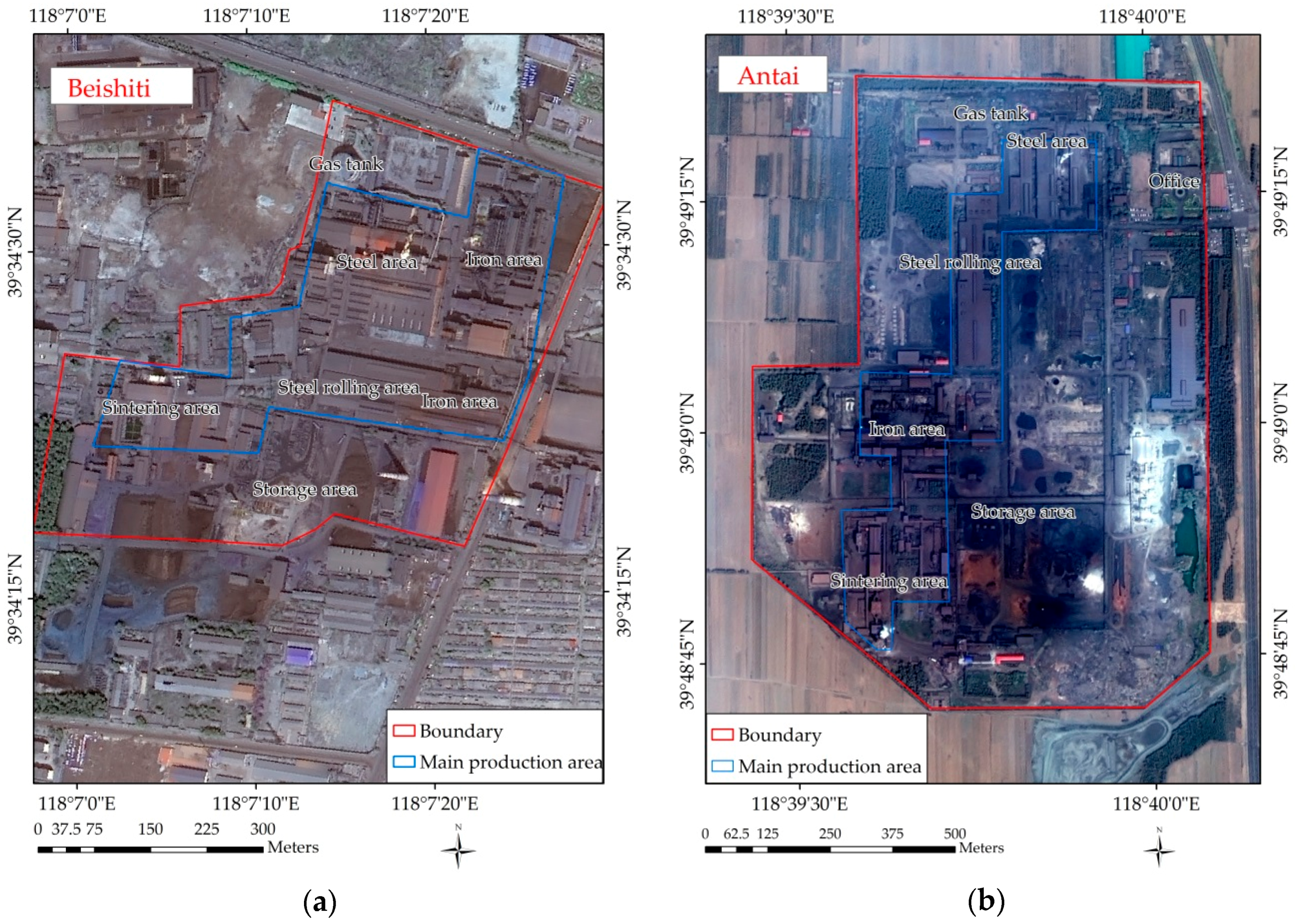
3.1.1. Identification of Main Functional Areas and Production Facilities

The GF-2 data were utilized to interpret the main functional areas and identify the typical facilities. According to the production process [44], an iron and steel factory is classified into at least nine functional areas via visual interpretation: storage area, sintering area, iron area, steel area, steel rolling area, gas tank, parking area, office area and power plant (Figure 6). For the basic functional areas, the functions and features are introduced as follows.

• Storage area: The production requires quantities of raw materials stored in the storage area. In some factories, reddish brown ore, black coal, and white limestone are piled in the open storage area [45].
• Sintering area: Sintering is the pretreatment of raw material. Generally, the functional area is close to the storage area, and these areas connected by a strip transfer channel. The dust vacuum machines have a cuboid shape on the remote sensing image, and they are often arranged in groups.
• Iron area: Ironmaking is an important sector of iron and steel production. The furnace is a typical marker indicating a complex independent building with a variety of connecting pipelines and plant equipment. The furnace chimney and cooling equipment can be observed. Generally, the number and volume of furnaces represent the production capacity of the factory.
• Steel area: The steel area is located close to the iron area with dense transportation [45]. The main facility has a converter and most equipment is installed inside the buildings.
• Steel rolling area: Rolling is the process of shaping the steel products through the use of rotating rolls, including hot and cold steel rolling.
• Gas tank: This equipment represents an important indicator of an iron and steel factory.
• Parking area: The open parking area for cars can reflect certain production conditions.
• Office area: The office area has independent buildings, with a tiny park or green areas.
• Self-provided power plant: In general, large iron and steel factories have their own power plants to recycle waste heat and gas heat with a white cooling tower.

According to the preceding definitions, the processes of sintering, ironmaking and steelmaking are the main sectors that generate most heat. Therefore, the internal area was divided into two types: the main production area (sintering area, iron area and steel area) and other area (Figure 7). These results are the basis for change detection and quantitative evaluation of the heat field change in an iron and steel factory.

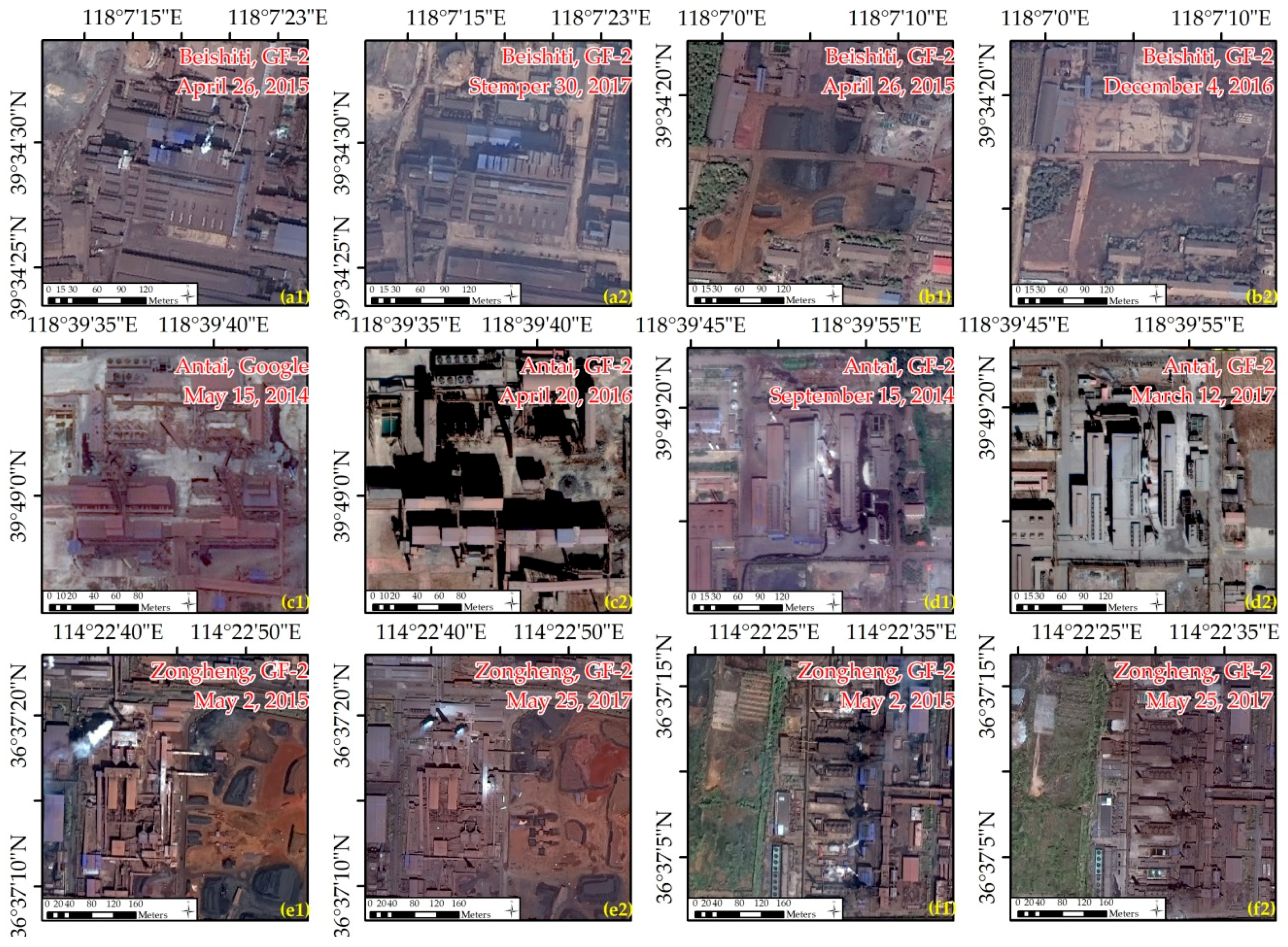
3.1.2. Change Detection on GF-2

Within a certain time series, surface facilities and land use change with the economic activity of an iron and steel factory, which cause regular variations in the internal heat field.

For the scale of the studied area, the method of visual interpretation with high accuracy [46] was used to detect how the surface facilities change. Focusing on the main production area, this approach aimed to obtain information regarding changes in the facilities or smog and generate precise evidence to verify the heat field analysis.

3.2. Quantitative Analysis of the Heat Field inside a Factory Based on LST

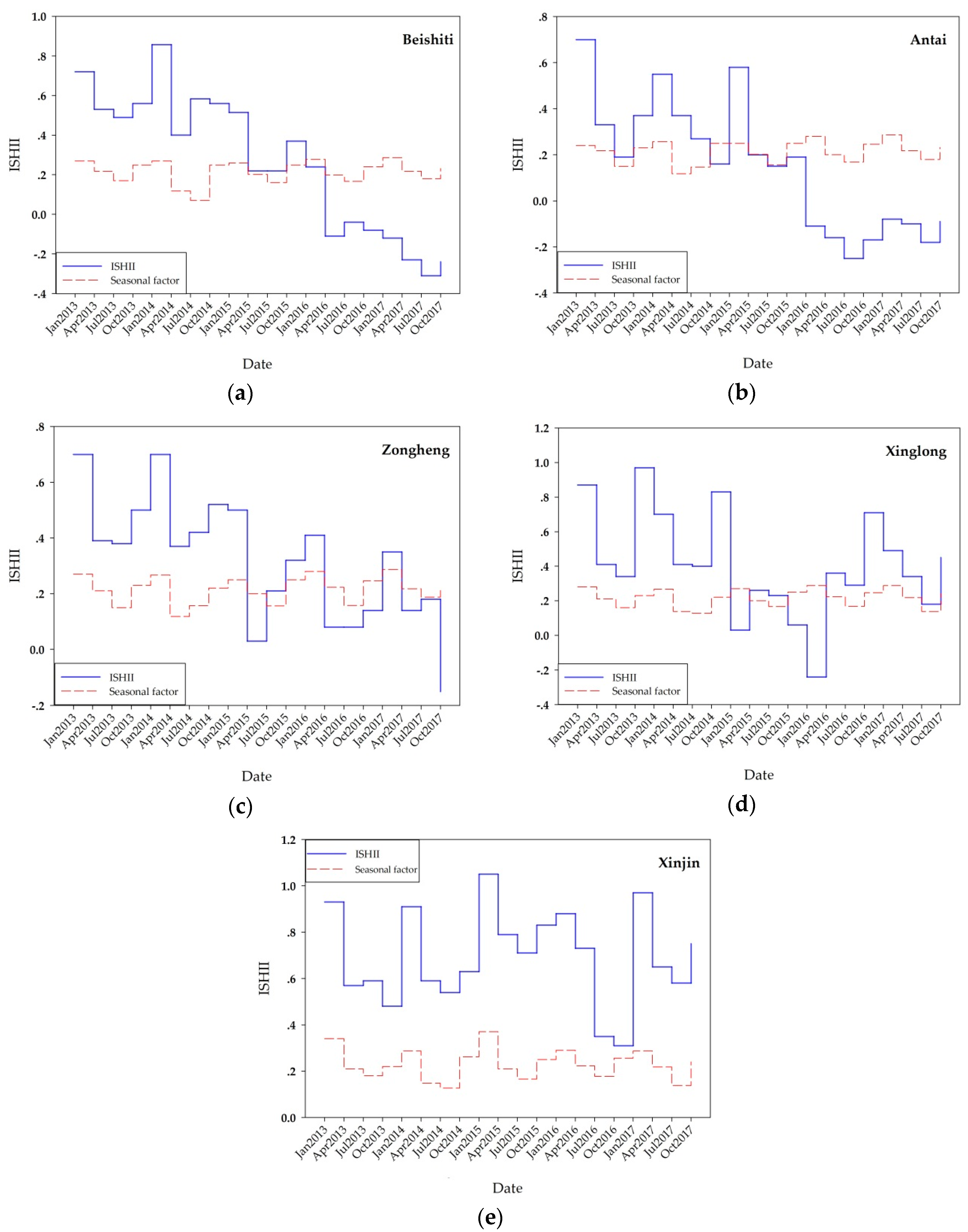
3.2.1. ISHII

Functional areas inside the iron and steel factory were classified into the main production area and other areas depending on the disequilibrium of heat distribution. The LST of the main producing area is higher than those of other areas, forming a relative heat island and cold island. Therefore, these features make it possible to monitor the economic activity of an iron and steel factory by quantitatively analyzing the LST differences between the two types of areas, even though LST is also affected by seasonal factors except production activities. Urban Heat Island (UHI) studies [19,47] provide some ideas.

The main production area was defined as a heat island named P1 and the other area was regarded as P2. The ISHII can be calculated as follows:

$$\mathrm{ISHII}=\overline{{\mathrm{LST}}_{\mathrm{P}1}}-\overline{{\mathrm{LST}}_{\mathrm{P}2}}$$

(10)

where $\overline{{\mathrm{LST}}_{\mathrm{P}1}}$ is the average temperature in the main production area and $\overline{{\mathrm{LST}}_{\mathrm{P}2}}$ is the average temperature in the other area.

Qing [27] noted that the UHI changed along with the season, with the smallest value observed in summer and the largest value observed in winter. Therefore, the ISHII was partly affected by seasonal variations. To allow fluctuating data to reflect real factory production changes, two points (on an outside road and the internal office building roof) near the iron and steel factory were chosen, and then the curve of the LST difference between these two points was calculated to represent the seasonal background.

3.2.2. ISHRI

For comparisons of thermal remote sensing data in a time series, a difference caused by seasonal factor leads to a considerable bias in evaluating the heat field [48], even if the internal production facilities or economic activities have not changed. Therefore, above-mentioned seasonal factor curve alone cannot eliminate seasonal effects accurately and it also cannot demonstrate the spatial changes of the heat field.

Because this study focused on the LST spatial distribution characteristics and the seasonal factors affect only the intensity of LST, the method of normalization [49] was used with the absolute LST (LSTa) to obtain the relative LST (LSTr) by incorporating all values into the range [0, 1] without changing the spatial distribution, as in Equation (5):

$${\mathrm{LST}}_{\mathrm{r}}=\frac{{\mathrm{LST}}_{\mathrm{a}}-{\mathrm{LST}}_{\min }}{{\mathrm{LST}}_{\max }-{\mathrm{LST}}_{\min }}$$

(11)

After normalization, the density classifying method was used to observe heat island transformations by classifying the LSTr image into different grades. In this study, there are six grades by the equal interval method in ArcGIS software from low to high: Grade 1 was defined as the low temperature area; Grade 2 was defined as the sub-low temperature area; Grade 3 was defined as the middle temperature area; Grade 4 was defined as the sub-high temperature area; Grade 5 was defined as the high temperature area; and Grade 6 was defined as the highest temperature area. Linked with the image on January 2013, the sub-high area (Grade 4), high area (Grade 5) and highest area (Grade 6) cover all production facilities in the steel enterprise as a heat island, whereas other grade areas are regarded as cold islands. The spatial changes of Grades 4–6 can represent the variations in the heat island of the iron and steel factory. The density classifying method was introduced to satisfy the requirements of the spatial analysis based on the internal heat island.

After performing the classification, Xu [30] proposed an urban heat island intensity ratio index [50] to evaluate the spatial changes of UHI. Based on this proposal, ISHRI is established in Equation (12) by calculating the relative area of the heat island. The values of ISHRI are used to quantitatively assess the variations in the heat island by determining the proportional relationship between the high temperature area and the changing spatial area.

$$\mathrm{ISHRI}=\frac{1}{100m}{\displaystyle \sum }_{i=1}^n{w}_i{p}_i$$

(12)

where m is the value of the total normalization grade; i is the grade of the temperature area; n is the number of temperature areas; w is the weight of grade i; and p is the proportionality of grade i. However, in our study, the parameters are stable in different periods of the images: m is 6; n is 3; w is 6, 5 or 4; and p is the area proportion of Grade 6, 5 or 4.

4. Results

Based on the above methods, the economic activity in the sample iron and steel factories can be measured from 2013 to 2017. Three types of economic activity were monitored, namely, normal production, shut down, and cut-back.

4.1. Time Series Analysis

The ISHII was used to identify changes in the economic activity of an iron and steel factory in a time series. The ISHII of each sample of the iron and steel factory was calculated from January 2013 to October 2017 in quarter intervals, as shown in Figure 8.

Combined with auxiliary information (Figure 5), a comparison of the ISHII curve with the curve of seasonal factors shows that ISHII is sensitive to the economic activity of the iron and steel factories. Overall, the changes of the ISHII in each quarter are consistent with the seasonal variations, although they show different features between each year under the de-capacity regulations. From 2013 to 2014, which represents the period when the economic activity of the iron and steel factory was not affected by government policy, the ISHII curve of the samples is normal and maintains a greater gap beyond the seasonal factors curve. Subsequently, from 2015 to 2017, the period with the strict control policy, the ISHII curve fluctuated dramatically.

For Beishiti, because of a cut-back, the gap between the two curves narrowed from April 2015 to April 2016; subsequently, the ISHII value was lower than the seasonal factor change under normal production. In approximately April 2016, Beishiti shut down all economic activity and the ISHII value decreased below 0.

For Antai, in October 2014, the ISHII value was lower than the seasonal factor change for the first time. This trend was inverted until January 2016, when the ISHII value decreased below the seasonal factor curve a second time and never recovered. According to the timelines of events, Antai went through two great changes in economic activity: a shut down and a return to production. When Antai shut down all production activity in January 2016, the ISHII curve decreased below 0.

For Zongheng, the ISHII curve fluctuates greatly. It was below the seasonal factor curve twice from April 2015 to April 2017, coinciding with two production stoppages. However, when production restarted, the inverse situation between the curves occurred from July 2015 to April 2016. After shut down in September 2017, the ISHII decreased below 0.

For Xinglong, the ISHII curve is below the seasonal factor curve twice from January 2015 to April 2016, when all economic activity was stopped. After restarting production, the ISHII curve exceeded the seasonal factor curve in April 2017 but it never achieved the previous level of 2013.

For Xinjin, with stable production activity, the ISHII curve always exceeded the seasonal factor curve. However, from July 2016 to January 2017, the ISHII value declines sharply because of a stoppage at several facilities. After continuous economic activity, the ISHII curve shows a high developing trend again in 2017.

In conclusion, the variations of the ISHII curve can reflect the economic activity in an iron and steel factory over time. When ISHII exceeds the seasonal factor change over the same time by a large gap, there is normal production; a narrow gap shows a cut-back; and, when the value of ISHII decreases below 0, it is verified that the entire factory has shut down.

4.2. Spatial Pattern Analysis

The density classifying method and ISHRI were used to understand the spatial pattern variations of the heat field inside the iron and steel factories from January 2013 to October 2017. The density classifying method directly describes the spatial transformation of heat island occurrence in images and ISHRI shows the heat island area changing quantitatively over the entire field of an iron and steel factory. An example of the LSTr and the graded distribution of Zongheng are shown in Figure 9.

As shown in Figure 10, the shrinkage of heat island areas was primarily concentrated in Beishiti, Antai and Xinglong from 2013 to 2017, whereas Zongheng and Xinjin presented limited changes except over a short period. The above results kept with the economic activity of the iron and steel factories: until October 2017, the ISHRI value in Antai and Zongheng was at a minimum, which is consistent with the change in production activities due to the shutdown; in this period, Xinjin and Xinglong were still in production with government permission. As the results indicate, the ISHRI can capture the spatial pattern changes of iron and steel factories to reflect their economic activity and monitor their changes in general.

However, from January 2016, the ISHRI of Beishiti increases sharply after the total shutdown and graded images in Figure 11 show that the heat island in Beishiti moved from the southwestern region to the southern region, which is not consistent with the actual situation because, during this period, the Tangshan World Expo was held, and Beishiti covered bare land with material that changed surface emissivity. Therefore, special situation should be noted by checking high-resolution images to determine whether land use has been changed.

4.3. The Changes Detection of Production Facilities

To explain and verify the analysis of the heat field accurately, detection based on high-resolution images from GF-2 and Google Earth was applied to production facilities changes during key periods. Figure 12 represented the main changes in the sample factories from 2014 to 2017.

For Beishiti, on 26 April 2015, this factory remained in stable production: Figure 12(a1,b1) shows that smog emitted from the sintering facilities and material remained in the storage area. However, from 2016 to 2017, the raw material in the storage area was cleared and raw material transport vehicles were not observed at the factory. From 2015 to 2017, no signs of production were observed for the Beishiti factory, as shown in Figure 12(a2,b2). For Antai, in 2014, two main blast furnaces remained and the production facilities were emitting smoke, as shown in Figure 12(c1,d1). However, one blast furnace was torn down, as shown in the image of 20 April 2016, and the associated facilities were shut down, as shown in Figure 12(c2,d2). The material heap in the storage area was greatly reduced; only a few piles of raw material were scattered and most of the area had been cleaned. Flue gas emissions were not observed in the sintering area and iron area, but the equipment and plant were intact and did not show signs of removal. For Zongheng, on 2 May 2015 the material in the storage area was abundant and the smog in the sintering area was heavy, as shown in Figure 12(e1,f1). On 25 May 2017, the raw material was unchanged and the smog in the sintering area was reduced, as shown in Figure 12(e2,f2). For Xinjin, normal production was observed on 23 May 2014, as shown in Figure 12(i1). A brief shutdown occurred on 25 July 2015 and in late 2016, and a decrease in smog is shown in Figure 12(g1,g2,h1,i2,i3). In April 2017, production was restored to the full working level, as shown in Figure 12(h2,i4). For Xinglong, the image on 25 September 2015 shows that most equipment had been shut down, and only a small amount of smog can be observed indistinctly. Certain equipment had been removed and the associated production had stopped, although parts of the facility were still working but with less smog, as shown in Figure 12(j1,k1). By February 2017, part of the equipment had returned to work but with much smog, as shown in Figure 12(j2,k2).

The changes detected via visual interpolation of production facilities revealed important changes in economic activity such as stopping the use of certain equipment and recovering production in a time frame. As a result, the change detection method provided detailed information on changes in smog and facilities on high-resolution optical images. It verified that constructed ISHII and ISHRI are effective indexes for reflecting and monitoring the economic activity of an iron and steel factory in a spatiotemporal series, and it provided powerful explanations for the variations of the internal heat field.

5. Discussion

Until December 2017, the Chinese Ministry of Environmental Protection had ordered local governments in major steel-producing cities to take tougher action against polluters from that industry as part of an effort to mitigate environmental pressures [51].

There are a few methods for monitoring and analyzing an iron and steel factory [6,52,53] before, but manual monitoring is discontinuous with spatiotemporal coverage and expensive. In addition, official statistical data on economic growth always has a large inaccuracy, especially when the iron and steel factory blindly pursue economy profit. Usually, the information acquired from remote sensors closely linked with iron and steel economic activity is more objective to reflect the change of production than official statistical data [18] and bear a lower cost. In this study, we first developed a satellite-based method for monitoring and detecting iron and steel factory economic activity that primarily includes normal production, shut-down and cut-back in five samples. Based on LST retrieved from Landsat-8 TIRS data, the heat island intensity of an iron and steel factory (ISHII) is used to monitor economic activity over time and the heat island ratio index of iron and steel factory (ISHRI) is used to reflect spatial changes. Then, the change detection method is utilized to obtain the surface facilities alternation by high resolution images of GF-2 and Google Earth in special time node, which finally aims at validation to ISHII and ISHRI.

From the time series analysis, the ISHII curve reflects the iron and steel factory economic activity. When the ISHII value exceeded the seasonal factor changes for a given time period, then the iron and steel factory was in normal production. If the gap decreased relative to that of the previous stage, the iron and steel factory had cut its production level. When the ISHII was lower than the seasonal factor changing, even lower than 0, the iron and steel factory had shut down. The ISHII index could explain the variations in intensity of the heat field.

From the spatial pattern analysis, the area and location of heat islands inside the factory were evaluated by the density classifying method and ISHRI. The density classifying method provided the spatial distribution of high and sub-high temperatures and showed how the heat island transferred. The ISHRI value evaluated changes in the production areas that occurred due to changes in thermal patterns. Generally, a high ISHRI value indicated dramatic economic activity. When the facilities do not change, the ISHRI still can provide powerful evidence to verify the economic activity of an iron and steel factory.

In addition, high-resolution images captured real information to explain and verify the analysis of the heat field in the iron and steel factory. Signs of smog, the amount of raw materials, and the entire state of the iron and steel factory represented different economic activities of production. Removing and shutting down facilities are significant causes of heat field changes. When the land use changed greatly after shutting down production, such as at Beishiti, the heat island may have been transferred to another location. This condition easily brings more bias in an ISHII or ISHRI evaluation, but change detection can reduce this error.

Therefore, the ISHII and ISHRI indexes and the change detection method can more accurately monitor economic activity. In pursuit of profit, some factories may ignore economic and environment policy to arrange production. Thus, this satellite-based method provides more accurate monitoring and comprehensive observation on an iron and steel factory from spatial and temporal series for economic growth and environmental sustainability. This study has expanded the application field of remote sensing and is the first to propose a satellite-based method for monitoring economic activity of an iron and steel factory as an economic object. Certainly, the real production data are not available for the sampled iron and steel factories to develop a quantitative relationship between the LST and production in our study. To increase the accuracy of economic activities evaluations, statistical data related to production should be included in future studies to improve the approach. In addition, based on the above study, there is potential for evaluating regional economic growth and development from the perspective of the iron and steel industry.

6. Conclusions

The study of iron and steel factories as important economic objects is indispensable for whole economic growth and environmental sustainability. However, traditional ground investigations with expensive cost cannot easily monitor spatiotemporal changes and statistical data are not accurate. Therefore, this study proposed a method for monitoring iron and steel factory economic activity based on satellites in a spatiotemporal series, which is also a new perspective for explaining economic activity. Internal heat field changes and surface facilities changes are measured using ISHII, ISHRI, dense classification and high-resolution images to monitor how the economic activity of the iron and steel factories changes in the spatiotemporal series. These objective monitoring results will be useful for promoting environment protection and adjusting industrial development. At the same time, it provides a new application based on satellites for monitoring economic activity and it is meaningful to deeply study economic sustainability via remote sensing technology.

References

1. Martinuzzi, A.; Blok, V.; Brem, A.; Stahl, B.; Schönherr, N. Responsible research and innovation in industry—Challenges, insights and perspectives. Sustainability 2018, 10, 702. [Google Scholar] [CrossRef]
2. Shatokha, V. The sustainability of the iron and steel industries in ukraine: Challenges and opportunities. J. Sustain. Metall. 2016, 2, 106–115. [Google Scholar] [CrossRef]
3. Shatokha, V. Environmental sustainability of the iron and steel industry: Towards reaching the climate goals. Eur. J. Sustain. Dev. 2016, 5, 289. [Google Scholar] [CrossRef]
4. Iron and Steel Industry in China. Available online: https://www.nytimes.com/2015/03/03/business/energy-environment/china-takes-on-steel-smog.html (accessed on 14 May 2016).
5. What China’s Steel Capacity Cuts Can Do for Iron Ore Prices. Available online: https://marketrealist.com/2017/03/analysts-expecting-iron-ore-prices (accessed on 1 February 2017).
6. Bo, X.; Zhao, C.L.; Wu, T.; Su, Y. Emission inventory with high temporal and spatial resolution of steel industry in the Beijing-Tianjin-Hebei Region. China Environ. Sci. 2015, 8, 2554–2560. [Google Scholar]
7. Ouma, Y.O. Advancements in medium and high resolution earth observation for land-surface imaging: Evolutions, future trends and contributions to sustainable development. Adv. Space Res. 2016, 57, 110–126. [Google Scholar] [CrossRef]
8. Justice, C.O.; Vermote, E.; Townshend, J.R.; Defries, R.; Roy, D.P.; Hall, D.K.; Salomonson, V.V.; Privette, J.L.; Riggs, G.; Strahler, A. The moderate resolution imaging spectroradiometer (MODIS): Land remote sensing for global change research. IEEE Trans. Geosci. Remote Sens. 1998, 36, 1228–1249. [Google Scholar] [CrossRef]
9. Gaur, A.; Eichenbaum, M.K.; Simonovic, S.P. Analysis and modelling of surface Urban Heat Island in 20 Canadian cities under climate and land-cover change. J. Environ.Manag. 2018, 206, 145–157. [Google Scholar] [CrossRef] [PubMed]
10. Yuan, G.-L.; Sun, T.-H.; Han, P.; Li, J. Environmental geochemical mapping and multivariate geostatistical analysis of heavy metals in topsoils of a closed steel smelter: Capital Iron & Steel Factory, Beijing, China. J. Geochem. Explor. 2013, 130, 15–21. [Google Scholar]
11. Zhao, H.; Ma, Y.; Chen, F.; Liu, J.; Jiang, L.; Yao, W.; Yang, J. Monitoring quarry area with Landsat long time-series for socioeconomic study. Remote Sens. 2018, 10, 517. [Google Scholar] [CrossRef]
12. Doll, C.N.; Muller, J.-P.; Morley, J.G. Mapping regional economic activity from night-time light satellite imagery. Ecol. Econ. 2006, 57, 75–92. [Google Scholar] [CrossRef]
13. Doll, C.H.; Muller, J.-P.; Elvidge, C.D. Night-time imagery as a tool for global mapping of socioeconomic parameters and greenhouse gas emissions. AMBIO 2000, 29, 157–162. [Google Scholar] [CrossRef]
14. Li, X.; Li, D. Can night-time light images play a role in evaluating the syrian crisis? Int. J. Remote Sens. 2014, 35, 6648–6661. [Google Scholar] [CrossRef]
15. Chinese Satellite Manufacturing Index (SMI). Available online: https://spaceknow.com/china/ (accessed on 3 April 2017).
16. Mert, M.S.; Dilmaç, Ö.F.; Özkan, S.; Karaca, F.; Bolat, E. Exergoeconomic analysis of a cogeneration plant in an iron and steel factory. Energy 2012, 46, 78–84. [Google Scholar] [CrossRef]
17. Liu, Y.; Hu, C.; Zhan, W.; Sun, C.; Murch, B.; Ma, L. Identifying industrial heat sources using time-series of the VIIRS Nightfire product with an object-oriented approach. Remote Sens. Environ. 2018, 204, 347–365. [Google Scholar] [CrossRef]
18. Ma, P.; Dai, X.; Guo, Z.; Wei, C.; Ma, W. Detection of thermal pollution from power plants on China’s eastern coast using remote sensing data. Stoch. Environ. Res. Risk Assess. 2017, 31, 1957–1975. [Google Scholar] [CrossRef]
19. Oke, T.R. City size and the urban heat island. Atmos. Environ. 1973, 7, 769–779. [Google Scholar] [CrossRef]
20. Lo, C.P.; Quattrochi, D.A.; Luvall, J.C. Application of high-resolution thermal infrared remote sensing and GIS to assess the urban heat island effect. Int. J. Remote Sens. 1997, 18, 287–304. [Google Scholar] [CrossRef] [Green Version]
21. Li, Z.-L.; Becker, F. Feasibility of land surface temperature and emissivity determination from AVHRR data. Remote Sens. Environ. 1993, 43, 67–85. [Google Scholar] [CrossRef]
22. Sobrino, J.; El Kharraz, J.; Li, Z.-L. Surface temperature and water vapour retrieval from modis data. Int. J. Remote Sens. 2003, 24, 5161–5182. [Google Scholar] [CrossRef]
23. Sobrino, J.A.; Jiménez-Muñoz, J.C.; Paolini, L. Land surface temperature retrieval from Landsat TM 5. Remote Sens. Environ. 2004, 90, 434–440. [Google Scholar] [CrossRef]
24. Jiménez-Muñoz, J.C.; Sobrino, J.A.; Skoković, D.; Mattar, C.; Cristóbal, J. Land surface temperature retrieval methods from Landsat-8 thermal infrared sensor data. IEEE Geosci. Remote Sens. Lett. 2014, 11, 1840–1843. [Google Scholar] [CrossRef]
25. Van der Meer, F.; Hecker, C.; van Ruitenbeek, F.; van der Werff, H.; de Wijkerslooth, C.; Wechsler, C. Geologic remote sensing for geothermal exploration: A review. Int. J. Appl. Earth Observ. Geoinf. 2014, 33, 255–269. [Google Scholar] [CrossRef]
26. Saraf, A.K.; Choudhury, S. Thermal remote sensing technique in the study of pre-earthquake thermal anomalies. J. Ind. Geophys. Union 2005, 9, 197–207. [Google Scholar]
27. Meng, Q.; Zhang, L.; Sun, Z.; Meng, F.; Wang, L.; Sun, Y. Characterizing spatial and temporal trends of surface urban heat island effect in an urban main built-up area: A 12-year case study in Beijing, China. Remote Sens. Environ. 2018, 204, 826–837. [Google Scholar] [CrossRef]
28. Chen, X.-L.; Zhao, H.-M.; Li, P.-X.; Yin, Z.-Y. Remote sensing image-based analysis of the relationship between urban heat island and land use/cover changes. Remote Sens. Environ. 2006, 104, 133–146. [Google Scholar] [CrossRef]
29. Weng, Q.; Lu, D.; Schubring, J. Estimation of land surface temperature–vegetation abundance relationship for urban heat island studies. Remote Sens. Environ. 2004, 89, 467–483. [Google Scholar] [CrossRef]
30. Xu, H.Q.; Chen, B.Q. An image processing technique for the study of urban heat islandchanges using different seasonal remote sensing data. Remote Sens. Technol. Appl. 2003, 18, 129–133. [Google Scholar]
31. Zhou, W.; Huang, G.; Troy, A.; Cadenasso, M. Object-based land cover classification of shaded areas in high spatial resolution imagery of urban areas: A comparison study. Remote Sens. Environ. 2009, 113, 1769–1777. [Google Scholar] [CrossRef]
32. Zhao, S.; Wang, Q.; Li, Y.; Liu, S.; Wang, Z.; Zhu, L.; Wang, Z. An overview of satellite remote sensing technology used in China’s environmental protection. Earth Sci. Inform. 2017, 10, 137–148. [Google Scholar] [CrossRef]
33. Hu, X.; Weng, Q. Impervious surface area extraction from IKONOS imagery using an object-based fuzzy method. Geocarto Int. 2011, 26, 3–20. [Google Scholar] [CrossRef]
34. Beijing-Tianjin-Hebei Region. Available online: https://en.wikipedia.org/wiki/Jingjinji (accessed on 15 April 2016).
35. Landsat 8 Tirs Data. Available online: http://glovis.usgs.gov/ (accessed on 15 December 2016).
36. Yu, X.; Guo, X.; Wu, Z. Land surface temperature retrieval from Landsat 8 TIRS—Comparison between radiative transfer equation-based method, split window algorithm and single channel method. Remote Sens. 2014, 6, 9829–9852. [Google Scholar] [CrossRef]
37. Qin, Z.; Karnieli, A.; Berliner, P. A mono-window algorithm for retrieving land surface temperature from Landsat TM data and its application to the Israel-Egypt border region. Int. J. Remote Sens. 2001, 22, 3719–3746. [Google Scholar] [CrossRef]
38. Du, C.; Ren, H.; Qin, Q.; Meng, J.; Zhao, S. A practical split-window algorithm for estimating land surface temperature from Landsat 8 data. Remote Sens. 2015, 7, 647–665. [Google Scholar] [CrossRef]
39. Jiménez-Muñoz, J.C.; Cristóbal, J.; Sobrino, J.A.; Sòria, G.; Ninyerola, M.; Pons, X. Revision of the single-channel algorithm for land surface temperature retrieval from Landsat thermal-infrared data. IEEE Trans. Geosci. Remote Sens. 2009, 47, 339–349. [Google Scholar] [CrossRef]
40. Gf-2 Data. Available online: http://www.cresda.com/CN/ (accessed on 1 April 2018).
41. Sobrino, J.A.; Jiménez-Muñoz, J.C.; Sòria, G.; Romaguera, M.; Guanter, L.; Moreno, J.; Plaza, A.; Martínez, P. Land surface emissivity retrieval from different vnir and tir sensors. IEEE Trans. Geosci. Remote Sens. 2008, 46, 316–327. [Google Scholar] [CrossRef]
42. Qin, Z.H.; Li, W.J.; Xu, B.; Chen, Z.X.; Liu, J. The estimation of land surfaceemissivity for Landsat TM6. Remote Sens. Land Resour. 2004, 3, 28–33. [Google Scholar]
43. De-Capacity in Iron and Steel Industry of China. Available online: http://www.google.com (accessed on 12 September 2017).
44. Industrial Efficiency Technology Database. Available online: http://ietd.iipnetwork.org/ (accessed on 24 May 2016).
45. Chen, P.F.; Lu, L.; Zhu, H.Z.; Zhu, Y.Q.; Wang, Y. Research on the suitability of image at different resolutions for theidentification of steel enterprise using remote sensing. J. Geo-Inf. Sci. 2015, 17, 1119–1127. [Google Scholar]
46. Lillesand, T.; Kiefer, R.W.; Chipman, J. Remote Sensing and Image Interpretation; John Wiley & Sons: Hoboken, NJ, USA, 2014. [Google Scholar]
47. Li, H.; Zhou, Y.; Li, X.; Meng, L.; Wang, X.; Wu, S.; Sodoudi, S. A new method to quantify surface urban heat island intensity. Sci. Total Environ. 2018, 624, 262–272. [Google Scholar] [CrossRef] [PubMed]
48. Kim, H.H. Urban heat island. Int. J. Remote Sens. 1992, 13, 2319–2336. [Google Scholar] [CrossRef]
49. Dodge, Y. The Oxford Dictionary of Statistical Terms; Oxford University Press: Oxford, UK, 2003; ISBN 0-19-920613-9. [Google Scholar]
50. Agam, N.; Kustas, W.P.; Anderson, M.C.; Li, F.; Neale, C.M. A vegetation index based technique for spatial sharpening of thermal imagery. Remote Sens. Environ. 2007, 107, 545–558. [Google Scholar] [CrossRef]
51. More Industrial Overcapacity to be Cut for High-Quality Economy in 2018. Available online: http://www.chinadaily.com.cn (accessed on 12 April 2018).
52. Duan, W.J.; Lang, J.L.; Cheng, S.Y.; Jia, J.; Wang, X.Q. Air pollutant emission inventory from iron and steel industry in Beijing-Tianjin-Hebei Region and its impact on PM2.5. Environ. Sci. 2018, 14, 1–14. [Google Scholar]
53. Liu, Y.J.; Ding, H. Variation in air pollution tolerance index of plants near a steel factory: Implication for landscape-plant species selection for industrial areas. WSEAS Trans. Environ. Dev. 2008, 4, 24–32. [Google Scholar]
Figure 1. Main flow of this study.
Sustainability 10 01935 g001
Figure 2. Location of the sample factories.
Sustainability 10 01935 g002
Figure 3. LST retrieved from Landsat-8 TIRS in Zongheng.
Sustainability 10 01935 g003
Figure 4. The preprocessing flow of GF-2.
Sustainability 10 01935 g004
Figure 5. Timeline of events for the five factories.
Sustainability 10 01935 g005
Figure 6. Main functional area.
Sustainability 10 01935 g006aSustainability 10 01935 g006b
Figure 7. Main production areas of the five factories. (a) is the map of main production area in Beishiti; (b) is the map of main production area in Antai; (c) is the map of main production area in Zongheng; (d) is the mao of main production area in Xinglong; (e) is the map of main production area in Xinjin.
Sustainability 10 01935 g007aSustainability 10 01935 g007b
Figure 8. ISHII of the sample factories from January 2014 to October 2017. (a) is the map of two curves of ISHII and seasonal factor changing in Beishiti; (b) is the map of two curves of ISHII and seasonal factor changing in Antai; (c) is the map of two curves of ISHII and seasonal factor changing in Zongheng; (d) is the map of two curves of ISHII and seasonal factor changing in Xinglong; (e) is the map of two curves of ISHII and seasonal factor changing in Xinjin.
Sustainability 10 01935 g008
Figure 9. Graded LSTr distribution of Zongheng: (a) 30 January 2014; (b) 17 January 2015; (c) 5 February 2016; and (d) 22 January 2017.
Sustainability 10 01935 g009
Figure 10. ISHRI of sample factories from January 2014 to October 2017.
Sustainability 10 01935 g010
Figure 11. Density classified images of Beishiti: (a) 5 May 2013; (b) 1 August 2016; and (c) 9 February 2017.
Sustainability 10 01935 g011
Figure 12. Surface changes in sample factories from January 2014 to October 2017.
Sustainability 10 01935 g012aSustainability 10 01935 g012b