Dynamically Controlled Length of Training Data for Sustainable Portfolio Selection

Abstract

In a constantly changing market environment, it is a challenge to construct a sustainable portfolio. One cannot use too long or too short training data to select the right portfolio of investments. When analyzing ten types of recent (up to April 2018) extremely high-dimensional time series from automated trading domains, it was discovered that there is no a priori ‘optimal’ length of training history that would fit all investment tasks. The optimal history length depends of the specificity of the data and varies with time. This statement was also confirmed by the analysis of dozens of multi-dimensional synthetic time series data generated by excitable medium models frequently considered in studies of chaos. An algorithm for determining the optimal length of training history to produce a sustainable portfolio is proposed. Monitoring the size of the learning data can be useful in data mining tasks used in the analysis of sustainability in other research disciplines.

1. Introduction

Changes in social, economic, technical, and political environments are everywhere in today’s rapidly developing world. Therefore, one of the requirements for modern decision-making systems is the ability to withstand sudden changes. Terms related to sustainability such as ‘maintain’, ‘support’, and ‘endure’ have become very important in such circumstances. Sustainability issues influence business in all industrial sectors and parts of the world, especially in marketing and management [1,2].

Financial portfolio management greatly affects industry, social life, and politics. The nature of multidimensional time series is determined by the interaction of millions of economic and financial units. Many unforeseen external consequences of political, environmental, meteorological, and natural disaster events also affect historical time series.

In the portfolio construction problem, people seek to allocate assets (stocks, bonds) in such a manner that it would maximize return given a fixed level of risk or reduce risk given a desired return. Currently, different investors use diverse algorithms for portfolio design. In computerized approaches, instead of assets, investors use automated trading strategies (ATS) as inputs for their portfolios [3,4].

There are several dozen formulations of what makes an optimal financial portfolio. Conventionally, a financial portfolio of assets is developed. Trading strategy can have a long, short, or flat position at any time. The position can change at any time during a day and sometimes even several times during the day. Typically, we record profit or loss (PnL) at the end of the trading day when the exchange closes. PnL is the profit difference from the same time in the previous business day. In US terms, that is at 4:00 p.m. Eastern Time. We use mark-to-market profit calculation methodology where we include all unrealized profits in our PnL.

In algorithmic trading, portfolio construction seeks to allocate money to different ATSs so that the resulting risk reward ratio is optimized. The biggest challenge in any portfolio construction is that portfolio results in the future or in the unseen data are often worse than was expected from historical results. This problem is even more acute in algorithmic trading as there is a far greater number of ATS than assets being traded by ATS, and classic portfolio construction methods are not suitable for this task.

This paper deals with the selection of a subset of portfolio inputs from a large investment universe. In the second section of the paper we present definitions and terminology used in the portfolio selection task and a literature review. In the third section we analyze ten types of recent high-dimensional financial time series with the aim of discovering which length of the most recent historical data is best to use for optimal ATSs selection. We discovered that there is no a priori fixed ‘optimal’ length of training history for all portfolio design tasks. It varies between two and 24 months. The most profitable training data length (TDL) can be estimated empirically by examining the prior successes of a set of potentially lucrative lengths. Consequently, we suggested and verified a simple algorithm for determining the optimal length of training history to produce a sustainable portfolio. The varying training data length phenomenon was confirmed in the third section’s analysis of a dozen multi-dimensional synthetic time series generated by an excitable medium model, frequently considered in studies of chaos.

2. Terminology and the Literature Review

The term “portfolio” refers to any combination of financial assets or ATSs. The idea is to put such ATS together so that if one ATS generates a loss during a day there will be other ATS that generates a profit and will compensate the loss of the first one. The main objective of developing a financial portfolio is to determine the N investment proportions, w₁, …, w_N, where the sum ${\displaystyle \sum _{j=1}^N{w}_j}=1,$ and all components, w_j, are positive. Denote r = [r₁, r₂, …, r_N], a N-dimensional vector of returns (profit or losses) of N investment assets or ATSs. Thus the portfolio profit is expressed as the weighted sum, P(r,w) = ${\displaystyle \sum _{j=1}^N{w}_j{r}_j}.$ If L vectors, r, are used as a training set, one can seek for the vector’s w, optimal proportions, where profit and risk are taken into account. We consider the problem of portfolio selection within the classical Markowitz mean-variance framework. To find the investment proportions, w₁, …, w_N, we have to maximize selected performance measure of the portfolio. We used standard mean-variance quality criterion (MVQC) [5,6,7]

$$MVQC(r)=mean\left(P(r)\right)/stdev\left(P(r)\right)$$

(1)

where mean and stdev denote a mean and a standard deviation or probability distribution of the returns.

In criterion (1) the profit and risk are taken into account. To evaluate mean and stdev one needs to know N-dimensional mean vector, and N × N-dimensional covariance matrix composed of N variances and N × (N − 1)/2 correlations. Criterion (1) is good when probability distribution of portfolio sums, P(r,w), is Gaussian and one knows the exact values of the means, variances, and correlations. Moreover, these values must not change in time. These requirements are very restrictive. In spite of sub-optimality, after more than half a century since the seminal work by Markowitz [5], the mean-variance framework remains prevalent and represents the most broadly chosen approach in both industry and academia for portfolio selection (see review [8]).

To mitigate the restrictive requirements, thousands of modifications of the mean/variance rule appear in the literature [8,9,10]. A number of papers were aimed to use other criteria than mean/variance ratio, such as requirements for maximal size of the portfolio, minimum position size, transaction costs, preferences over assets, management costs, etc. Methods were created to take into account the skewness and kurtosis of the asset distribution [9]. In an attempt to take into account the variability of data, a number of papers have been devoted to efficient managing of temporal information [11,12]. Use of meta-heuristics for increasing the speed of optimization methods of ratio (1) in high-dimensional situations have been suggested as well [10].

In analysis of sustainability it is very important to consider learning set size—portfolio dimensionality effects [13,14]. In a previous paper [14], an expected value of the mean sample MVQC criterion was investigated in an asymptotic where both the learning set size, L, and portfolio dimensionality, N, were increasing, however, ratio L/N does remain constant. This approach allowed for the obtaining of an explicit asymptotic equation to calculate the out-of-sample MVQC criterion

$$MVQ{C}_{\mathrm{out}-\mathrm{of}-\mathrm{sample}}^{}\to \delta /\sqrt{T_{mean}\times T_{\mathrm{var}}}.$$

(2)

where δ is a limiting value of ratio (1) when L tends to infinity, however N is fixed;

T_mean = 1 + N/(L × δ²),

(3)

T_var = 1 + N/(L − N).

(4)

Term (3) is responsible for the inexact estimation of the mean vector of returns and term for inexact estimation of correlations. Theoretical and experimental analysis showed [14]:

-

Estimation of variances asymptotically does not affect the $MVQ{C}_{\mathrm{out}-\mathrm{of}-\mathrm{sample}}^{}$ value;

-

if L < N, we cannot estimate CM.

Term (3) demonstrates that estimation of several thousands of components of the mean vector makes the learning set-based portfolio ineffective. Suppose, N = 6000, δ = 0.5, and L→∞. If L = 256, use of term (3) leads to MVQC = 0.052. An extraordinary difference between these values indicates that in an inexact estimation the mean return values reduce the MVQC criterion almost ten times!

Thus, for situations where learning set size is small and dimensionality is high, the classical criterion (1) becomes useless. A number of simplifications for estimation of the covariance matrix have been suggested: regularization, subset resampling, splitting the portfolio inputs matrix into a lot of parts, etc. [15,16,17,18].

A limiting case for simplification of the portfolio construction is a non-trainable 1/N rule where all N portfolio inputs are weighted equally. In many cases, the 1/N strategy can become the most effective one [19]. In this rule, the portfolio optimization (training) consists of selecting a subset of assets or the trading strategies from an investment universe with respect to a given portfolio performance criterion. Nowadays, the selection problem becomes very important since the number of trading strategies and stocks listed on stock markets are continuously increasing [20]. A number of algorithms and criteria for stock screening and ranking are proposed in the literature [21,22,23].

An important factor in the application of stock screening and ranking algorithms is the size of the data used to estimate numerical effectiveness values. In a previous paper [24] the authors examined the financial portfolio inputs’ random selection optimization model. We derived an equation to calculate an accuracy of the out-of-sample MVQC criterion value in dependence of the number of potential asset number of portfolio inputs, N₀, the desirable portfolio size, N (N₀>>N₀), the sample size L used to estimate MVQC criterion and complexity of the random search procedure (a number of times, m, the portfolio subsets were generated randomly). It was demonstrated that with an increase in portfolio complexity and complexity of optimization procedure, m, we can observe the over-fitting phenomena in the selection procedure. For this reason, often one employs simple selection rules such as selection of the individually most effective inputs [20,23,25,26].

Informative learning set size is closely related to environment changes. If environmental changes are frequent, only short historical data segments turn out to be reliable. Hence, the small sample problems are very important in sustainability analysis. To explore and understand the almost chaotic ceaselessly changing environments in financial portfolio management it is necessary to comprehend training data length/complexity relations of portfolio design rules.

To the best of our knowledge, learning set size problems arising in chaotically changing financial data were not considered in the literature. As an exception we can mention an attempt to determine training history length using a relatively small number of potential ATSs (N₀ = 169) [15]. It was found that the length should be rather short, 500–600 business days. To cognize sustainability issues one needs to analyze regularities of financial chaos by considering not a single, but a wide diversity of real world data sets. In order to better understand stability problems, it is also necessary to use ideas from chaos theory [27,28], e.g. explore synthetic purely chaotic multi-dimensional time series in which external unforeseen events do not affect the created time series.

3. The Methodology

Our research is pointed towards designing a sustainable portfolio management strategy that can endure for a long time in the chaotic, ceaselessly changing environment. An important step in our research is to find the training data length to be used to design the financial portfolio. Obviously, it depends on the frequency and magnitude of environmental changes. In Section 2 we reviewed our earlier analytical results concerning the influence of learning set size on mean-variance principle designed portfolio [14] and random search based best input selection [24]. These results were obtained for static situations. For chaotically hanging environments, however, we have no means to perform analytic investigations. For that reason, we need to perform experiments with a large number of diverse types of real world financial data stored in financial databases. In order to expand sustainability issues to wider research disciplines a part of the experiments we performed with synthetic chaotic data.

3.1. Financial Data Used

Automated trading is when a human writes a computer algorithm that can trade in financial markets automatically, by using predefined rules. These algorithms are called Automated Trading Strategies (ATS). For example, ATS can buy and sell Apple stock based on stock price changes. Individual ATS on a given day can make or lose money, though in the long term, the results are positive. The aim is to put several ATS in a sustainable portfolio in such a way that if one ATS loses there will be another to make money on that day. The more independent ATS we put together, the better the result. The problem is to find independent, sustainable, and consistent ATS that do not change their behavior in the future.

Given ATS, one can execute computer algorithms in simulations and see how well the ATS would have performed on historical data. The results of this simulation can be recorded, analyzed, and used to design a portfolio composed of several ATS. Typically, one records daily profit and loss (PnL) of ATS. That is how much money ATS made or lost during that day. We investigated the daily series of PnLs of fifteen years, from 2003 to 2018. This data was given to us by trading firm that uses these ATS in practice.

PnL is the amount of US dollars made or loss during a day. ATS PnL is a series of daily profit and losses from 2003 to 2018. Portfolio PnL refers to a sum of ATS PnLs—every day, we sum profits and losses from all ATS in the portfolio and that constitutes portfolio PnL for one day.

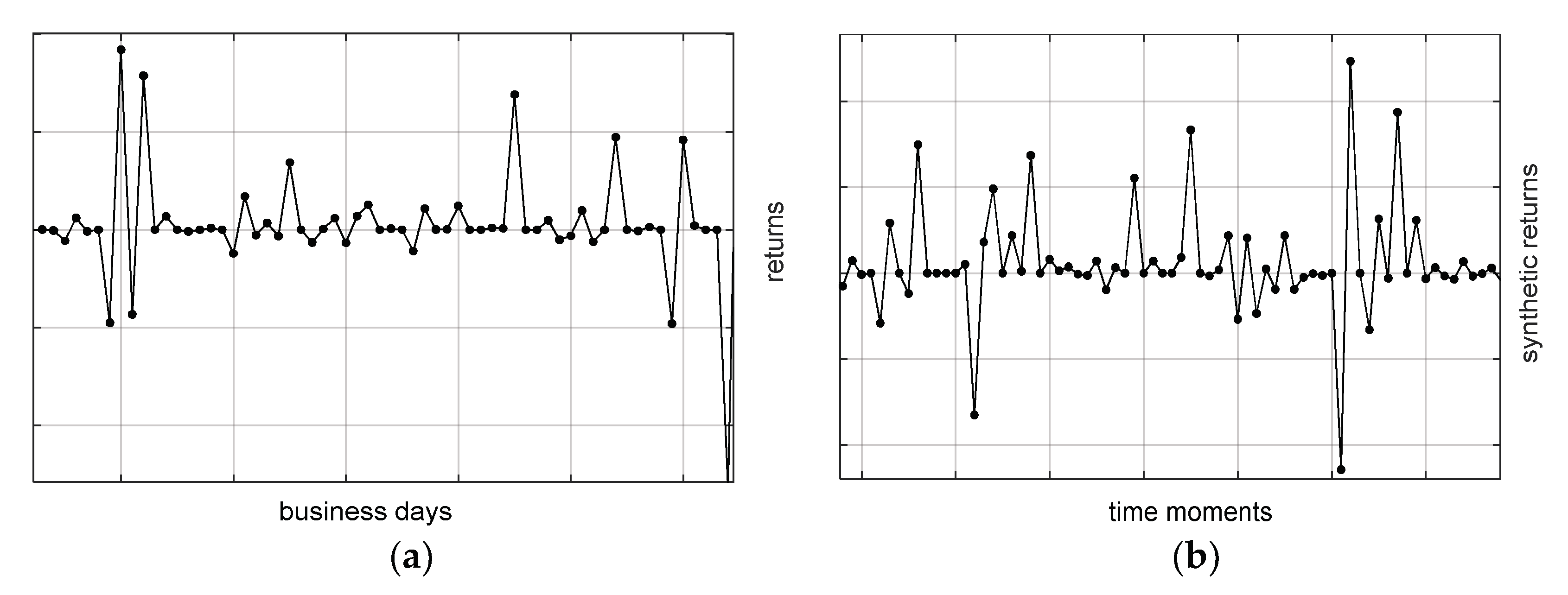
ATS can be very different from each other. There are many different rules that can be put into a computer algorithm. Our data consisted of mainly 3 types of ATS: Mean reversion (MR), Trend following (TF), and Event-based Trend (ET). In automated trading often one uses ATS strategies where strategies differ in the investment risk levels that lead to frequent refusal from investments. In the case of refusal, the next day’s return is equal to zero (see Figure 1a). For more details about the data see Appendix A.

3.2. Preparation of the Financial Data and the Experiments’ Design

We consider the algorithmic trading where the number of ATS (a maximal portfolio dimensionality) can be as high as N₀ = 258,000. In such situations we are obliged to reduce the dimensionality of the portfolio inputs drastically. At the same time, we have to use only the simplest, the 1/N portfolio rule.

In the investigation of the dynamic portfolio selection scheme, we assigned two years history data allocated for “comparison of diverse lengths of training data”. The next month is assigned for out of sample testing, i.e., for calculating the returns of each day. We aimed to determine the best training data length and to select N_portfolio ATS for the 1/N portfolio design. In the experiments we moved stepwise the 25 month data segment 1 month forwards until the data history end. During each single step we estimated the MVQC ratio for all N₀ ATSs M = 6 times with 2, 4, 9, 12, 18, and 24 month training data histories. Then for each training set size we selected N_portfolio = 10 best trading strategies and used them for calculation profits or losses for all business days of the test month.

Procedure “select the individually best ATSs” is the simplest and fastest one among a many selection rules used in data mining tasks. One of heuristic procedures employed in the portfolio selection is a Comgen rule [15,29] where the best ATS, say the j-th one, is selected first, then all N₀ (N₀ − 1)/2 pairs containing the j-th ATS are compared and then the best pair is selected. The selection process goes on until N_portfolio ATS are selected. To evaluate performance of the set N_portfolio trading strategies in the “individual selection” procedure we have to estimate N_portfolio means and N_portfolio standard deviations of the returns. A simple matrix algebra shows that in the Comgen procedure it is additionally necessary to estimate N₀ × (N₀ − 1)/2 correlation coefficients. Therefore, the Comgen procedure is more complex and requires longer training set sizes. Theoretical and empirical investigations [24] show that in a small sample size situation simpler procedures like “select individually the best ATS” are more preferable when sample size is small (two months data, 41 days).

Preliminary experiments showed that often even four month training data can be too long for portfolio selection in frequently changing situations. Often the ATS selection based on two months of data outperformed the portfolio based on four months of data. It is a frustrating truth in the situation when we have 15 years of historical financial data at our disposal. These conclusions prompted us to devise a new approach to employ lengthy historical data.

In an attempt to use the information contained in the older data, we divided the 15 years of data sets into two parts. The first part of the data of each dataset (up to 1 January 2011) was assigned for preliminary subset selection (PSS) used for formation of N₁-dimensional subset of the most profitable trading strategies (typically N₁<<N₀). The conventional way to select N₁ best trading strategies is to use the first part of the data to estimate the MVQC ratio of all N₀ ATS. Then one selects N₁ ATS with the highest MVQC ratio values. This procedure we will name PSS1.

Our novel stepwise procedure (PSS2) is based on an assumption that due to unexpected environmental changes, different ATS should be specific to be profitable at various short time intervals. Contrary, the procedure PSS1 selects nonspecific (indistinct) trading strategies. The procedure PSS2, however, is more complex. Having 8 years (96 months) of historical data we considered 95 two month-length time series sections to estimate the MVQC ratio of N₀ trading strategies and select n₁ = 70 best of them to be included into subset PSS2. We will have to repeat the selection process many times. Therefore, procedure PSS2 is slower. In columns “Dimension” and “Reduced dim” of Appendix A,

Table A1. Description of the real world data used in this study.

No	Date	Type	Dimension	Reduced Dimens.	All ATS Max/End	Reduced, SS2 Max/End	Abr.
1	20180319	MRS	50,194	4681	63/51	99/82	D50
2	20180320	MRS	257,769	4023	38/32	98/97	D258
3	20180320	MR	44,068	3533	66/66	102/97	D44
4	20180326	MR	104,204	3751	85/85	67/67	D104
5	20180329	ET	56,197	4641	38/38	35/26	D56
6	20180412	TM	66,897	2769	93/79	81/69	D67
7	20180415	MR	49,622	1927	27/27	44/41	D49
8	20180401	ET	18,703	4448	182/162	135/78	D19
9	20180412	MRS	178,602	3422	97/88	142/104	D178
10	20180421	MRS	102,251	3379	52/52	46/46	D102

we present values of N₀ and N₁ for ten data sets used in the experiments. For each data set the number N₁ was determined individually using the procedure PP2.

In the experiments with ten data sets we observed high influence of environmental changes on the “optimal” training history time. Therefore, the investor-practitioner is obliged to find most effective training period. Possible algorithms will be presented in the subsequent section.

4. The Analysis of Financial Time Series

To make conclusions authoritative, we prepared ten brand new (until April 2018) large scale sets of the financial data. In the experiments, we examined the successes of M = 6 portfolios based on the training data of six different lengths (2, 4, 9, 12, 18 and 24 months). We fixed the dimension of the portfolio, N_portfolio, a priori. The value N_portfolio = 10 was set up after a large number of previous (2015–2016 years) experiments performed with other sets of financial ATS data.

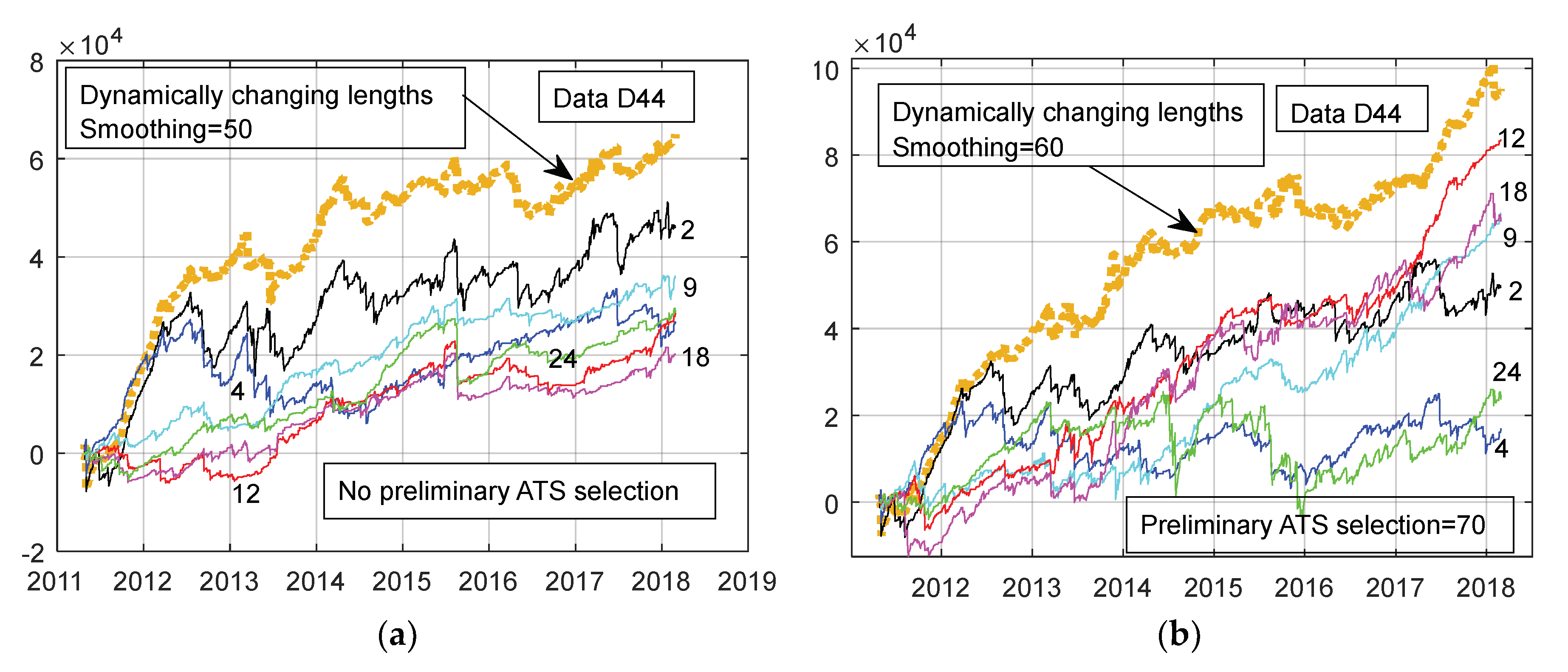
Figure 2a,b show six curves: “variation of the cumulative sums of portfolio PnL in time”, CS1, CS2, ..., CS6. Each of them corresponds to a diverse length of the training data. Curves in Figure 2a correspond to experiment when the best N_portfolio ATS were selected out of N₀ = 44,068 original trading strategies of 44,068–D (dimensional) data set D44. We see that the best learning set size was 2 months (curve 2 in the figure). Training set sizes of 12, 18, and 24 months in length resulted in the worst results. Better portfolios were obtained in the situation when, for the final decision making, we selected dynamically from the pool PSS2 of 3533 specific trading strategies (Figure 1b). The two-month length training set was among the best up to the year 2017. In this time the four months training history was unsuccessful. One may guess that the third and fourth backward shifted training months are harmful for this data. In Figure 1b we see, however, that the 9–18 backward shifted training months were very useful during the year 2017. These observations lead to the conclusion that the most effective duration of training depends on time. This conclusion was confirmed in experiments with the rest of the data sets. Portfolio performances with nonspecific ATSs (pool PSS1) were similar to that as results without the primary ATS selection.

To design a profitable portfolio for each trading day, we need to know the optimal length of the training data. To fulfill this requirement for the z-th day we can analyze curves CS₁, CS₂, …, CS₆ up to the z-th day and decide which training data length was the most profitable during the past time period. To estimate the desirable TDL, we chose the simplest method: we smoothed the return curves with period Smoothing days, and selected the length corresponding to the highest return value. In practice, however, the best smoothing interval values are unknown. Hence, the investor is forced to examine carefully a history of past successes (the set of different smoothing values in the previous history up to the z-th day). In Figure 2a,b, we depicted a variation of cumulative sums of the 10-dimensional portfolio returns, when the length of the learning data was determined dynamically according to the rule described above (bold dark yellow doted curves). We see, in this example the dynamics TSL determination outperforms remaining six curves obtained for the six definite values of TDL. Thus, that the novel simple method works. Figure 2a,b demonstrates that the preliminary reduction of data D44 dimensionality performed on the basis of 2003–2010 year data lead to a visible increase in the final portfolio performance.

Analyzing the remaining nine arrays of financial data, we found frequent situations in which the two months’ history used to select the set of the most productive ten ATS were the best. Nevertheless, for some financial data, we observed a reverse scheme: the most profitable were the long histories of the training data. In Figure 3a,b we present such example (257,769-dimensional data set D258). Like in data set (D44) the dimensional reduction method PSS2 was profitable: the portfolio returns increased more than two times. The use of dynamically changing learning data is superior to portfolios that have been trained by 18 or 24 month periods. Data for 4 months of training was again less successful than the data for two months. However, in both cases it was useful to increase the length of the training data further.

Figure 3a shows that in period after June 2015 the dynamic control of the TDL stopped being effective. Recommendation: after observing such a phenomenon in the history of past successes, the investor must choose another, more profitable data set of financial time series immediately. In this example the choice is simple: after the 2016, one needs to use the data set D258 with specific 4023 trading strategies (see Figure 3b).

Due to the random nature of the data, the cumulative sum of the dynamically controlled portfolio returns, increases in a wavy manner. In the Appendix A, Table A1 we present cumulative sums of the N_portfolio-dimensional portfolio at its maximum and at the last day of the inspected data. It is done for the original N₀-dimensional data and for the PSS2 reduced dimensionality data. In 50% of cases primary dimensionality reduction with procedure PSS2 improved the 10-D portfolio selected directly from original N₀-dimensional data (an interested reader can find figures similar to Figure 2 and Figure 3 in a web page of Vilnius university: https://mif.vu.lt/aistis/2018/sustainability).

We tested the procedure PSS1 to reduce primary dimensionality of the data as well. In all cases, except D56 data, the method PSS2 outperformed method PSS1. For data D56 the PSS1 method resulted in cumulative sums of the portfolio returns 60/52 (60,000 at the maximum, and 52,000 for the last day of the data). It means that the novel stepwise dimensionality reduction procedure, PSS2, is worth investigating further. The results obtained advocate that efficacy of the dimensionality reduction algorithm, PSS2, depends on the data. Therefore, instead of the two-month data interval used to evaluate and select the N₁ best trading strategies at each step, shorter or longer time intervals can be used. Possibly, the go-forwards steps ought to be shorter than one month. Diverse values of N₁ should be investigated. A problem of improvement of the accuracy of training data length determination procedure is important for future research. One needs to examine the larger number, M, of training data sizes, L, and the smooth empirical curves according to the L direction.

5. The Analysis of Synthetic Chaotic Multi-Dimensional Time Series

5.1. Generation of Synthetic Chaotic Multi-Dimensional Time Series

To understand sustainability problems better, varying training set’s length phenomenon was used together with the excitable media model to generate and analyze a number of multi-dimensional synthetic time series data sets. In financial markets, thousands, if not millions, of active agents interact with each other. A popular model to simulate some chaotic phenomena is wave propagation in excitable media [30]; it is the general approach. It has been used in the analysis of the wave propagation in chemistry, biology, medicine, epidemiology, quantum physics, and astrophysics. The present model’s version was suggested in a previous paper [31].

In a two-dimensional multi-group model, we have a large amount of agents (nodes of the excitable media) where each agent can be excited by its neighbor in the group. After starting excitation (e.g., appearance of some important novel information, the investment, etc.) and small delay, the central agent of the group forwards its excitation signal to neighbor agents of the group (see Figure 4a illustration for two-dimensional hexagonal grid). The signal transmission delay is increased by the signal power. The delay and power of excitations to adjacent companion nodes depend on the sum of the strength of the node’s excitation. After transmitting a signal to its neighbors, each node (Agent) has to take a rest (the refractory period). After this period, the excitation signals are transferred to further nodes. In this way the excitation signal can start travel backwards as well. Depending on the model parameters (excitation signal threshold, delay, refractory period, a number of neighbors to be excited by the single node, excitation signal strengths, etc.) the excitation signal patterns can be circular, regular, or chaotic. In Figure 1b we see signal propagation pattern in the hexagonal excitable media model composed of 93,457 nodes, after 456 iterations for a certain set of the model parameters that ensure the regular signal propagation and a symmetric in six directions ornamentation. The excited nodes are depicted in black. Nodes in the refractory period are depicted in green. Looking at the Figure 4b from a distance we can observe replicating geometric patterns (fractals). Observing the small areas of the large agent excitation pattern, however, we see only chaotic behaviors (Figure 4c,d). This observation supports Peters [28] affirmation: most natural systems are characterized by the local randomness and global determinism.

Independence of the model parameters and the waves of signal propagation can cease at the very beginning, after a moderate number of time steps, or after overstepping the hexagonal borders of the grid. To avoid the ceasing of the excitation signals in our “chaos generating model” we created a number of separate groups (grids of nodes), and introduced a restricted level of cooperation between them. If a sum of node’s excitations in a defined subgroup of nodes (200 adjacent nodes) goes above a certain threshold, the agents of this group can transmit the excitation signal to the group in which excitation signals had almost ceased. In this way, the group model mimics a team at work. If the parameters of such a team are chosen properly, the excitation signals do not fade away. Inside each group we formed eleven large nonintersecting subgroups of adjacent nodes (agents). Sums of the excitations of the agents in the single node group were used as the components of the multidimensional time series, named A. Differences between two adjacent values composed time series B.

For convenience we name these differences as “PnL” and the time moments as “business days”. Like in above analysis or real world data, in analysis of the synthetic time series we introduced automatic trading strategies where strategies differ in the investment risk levels that lead to frequent refusal from investments. In the case of refusal, the next day’s return is equal to zero. This type of the time series is named as series C. In Figure 1b we show the single synthetic time series, C, measured during 60 time moments. The return graph is very similar to authentic returns graphs obtained in real automatic trading systems (see e.g., Figure 1b and Figure 1 in [32]).

5.2. Experimental Results

The main difficulty in creating synthetic datasets is often bifurcations, which can lead to the cessation of excitations and the loss of stability of individual components of time series. The experiments were carried out only with sustainable components of the time series. Therefore, we generated and tested many dozens of the multidimensional time series data sets. The experiments were carried using the same methodology and software as in examination of the financial data.

While testing numerous diverse synthetic data, generated for 3, 4, or 6 excitable media (diverse groups of the similar agents) having various sizes and model parameters we obtained families of graphs similar to curves presented in Figure 2 and Figure 3. The curves obtained showed clearly that cumulative sums of the “synthetic returns” depend on the length of training data. As an example we present the simplest model where the generation of high-dimensional chaos time series was composed of six groups of excitable media differing in size, 15,769, 14,077, 12,481, 10,981, 9,577, and 8,269 nodes and the parameters of all 71,154 nodes were identical. In Figure 5 we present four curves of cumulative sums of virtual portfolio returns designed for the synthetic data (black, blue, magenta, and cyan curves). We see in different time intervals different training data lengths, L, are preferable. Timely change of TDL from 9 virtual “months” (cyan curve), to 2 months (black) allowed for an improvement of the sustainability of the portfolio (bold red curve).

Similar results were obtained using synthetic time series modeled with dissimilar sets of parameters. It should be remembered that the generators of chaotic time series were not specifically aimed at imitating economic and financial phenomena. Nevertheless, simulation experiments confirm the phenomenon of the different lengths of the training set, observed earlier in the experiments with real financial data. This means that monitoring the size of the learning data can be useful in the data mining tasks used in the analysis of sustainability in other research disciplines.

6. Conclusions

In automated trading portfolio construction, we are faced with the task of how to select from hundreds of thousands of automated trading strategies. This is very important in a frequently changing environment. Changes in the economy and the financial environment necessitate the use of short training sets exploited to select a small subset of potentially beneficial ATS. Practitioners want to have simple empirical rules, such as ‘in daily trading we have to use the data history up to 12 months’. When analyzing ten large-scale sets of financial data sets and artificially generated multi-dimensional time series, we came to the following conclusions:

• In situations with a frequently changing economy and financial environment, it is impossible to develop a simple rule of thumb that would fit all investment tasks. In modern daily trading with ATS, the length of the training data should vary from two to 24 months.
• The useful training data length (TDL), L, depends on the task, namely the initial set of ATSs and the method used to reduce their dimensionality. It also depends on the frequency of chaotic and unexpected changes of the environment. Large-scale experiments have confirmed that a useful TDL changes over time, and this fact cannot be ignored by an investment practitioner. This is the main finding of the paper.
• Situations in which the time intervals between two adjacent changes in financial time series are long are not rare. In such cases, a thorough check of the relative effectiveness of using different TDLs during the previous period of time allows one to select the correct length of training data and increase the portfolio return.
• The conclusion regarding the change in profitable TDL was confirmed by numerous experiments with synthesized multidimensional time series of chaos generated without the inclusion of external excitation signals. The study of synthetic chaotic time series confirms the fact that monitoring the size of the learning data can be useful in the tasks of data mining used in the analysis of sustainability in other research disciplines.

These conclusions suggest the following recommendations for trading practitioners:

• Select a set of N₀ original ATS. Prepare the software that allows for generating lengthy history of N₀ returns, say, for the last 10–15 years.
• Prepare user-friendly software designed to pre-select a smaller subset of the most efficient ATS. The selection should be based on the history of the data for several years, as was done in the experiments described above. To estimate the effective TDL, use previous data histories to verify the efficacy of such procedures for the investor’s data set.
• Prepare the software aimed at performing the secondary selection of N_portfolio-dimensional subset of ATSs to be used for subsequent day trading. This time the ATS selection is performed according to L days of training data.
• These steps can be performed for each business day M times for each of training set size, L₁, L₂, …, L_M. In our experiments we considered M = 6 sizes of learning sets. We advise using the larger number in practical work.
• In practical trading, we need to smooth out the results of the M-series, analyze their behavior during the previous period, and then choose the most promising TDL for the day’s trade.

The procedure just described does not guarantee perfect and profitable investments for all types of data. When frequent environmental changes follow each other, all training set sizes can lead to losses. In such a situation, the investor is recommended to avoid trading with this particular type of data. To make one’s investments sustainable, one needs to choose a different set of ATSs. We see an example of this in Figure 2b, where data D44 is considered. In the portfolio governed by dynamically controlled TDL, the cumulative profit curve fell during period November 2015–May 2016. Looking at Figure 3b, where data D258 are considered, we see an increase in the cumulative sum of returns of dynamically controlled portfolio in the same period.

References

1. Pakseresht, A.C.; Mark-Herbert, C. A review of sustainable development in brand value assessments. Soc. Bus. 2016, 6, 219–247. [Google Scholar] [CrossRef]
2. Heising, W. The integration of ideation and project portfolio management—A key factor for sustainable success. Int. J. Proj. Manag. 2012, 30, 582–595. [Google Scholar] [CrossRef]
3. Araújo, C.; de Castro, P. Towards automated trading based on fundamentalist and technical data. In Advances in Artificial Intelligence; Springer: Berlin, Germany, 2010; Volume 6404, pp. 112–121. [Google Scholar]
4. Aldridge, I. High-Frequency Trading: A Practical Guide to Algorithmic Strategies and Trading Systems; John Wiley & Sons: New York, NY, USA, 2010. [Google Scholar]
5. Markowitz, H.M. Portfolio Selection. J. Financ. 1952, 7, 77–91. [Google Scholar]
6. Reilly, F.; Brown, K. Investment Analysis and Portfolio Management; Dryden Press: Hins-dale, IL, USA, 2011. [Google Scholar]
7. Baker, H.K.; Filbeck, G. Portfolio Theory and Management; Oxford University Press: Oxford, UK, 2013. [Google Scholar]
8. Kolm, N.; Tütüncü, R.; Fabozzi, F.J. 60 Years of portfolio optimization: Practical challenges and current trends. Eur. J. Oper. Res. 2014, 234, 356–371. [Google Scholar] [CrossRef]
9. Mansini, R.; Ogryczak, W.; Speranza, M.G. Twenty years of linear programming based portfolio optimization. Eur. J. Oper. Res. 2014, 234, 518–535. [Google Scholar] [CrossRef]
10. Di Tollo, G.; Roli, A. Metaheuristics for the portfolio selection problem. Int. J. Oper. Res. 2008, 5, 13–35. [Google Scholar]
11. Balvers, R.J.; Mitchell, D.W. Efficient gradualism in inter-temporal portfolios. J. Econ. Dyn. Control. 2000, 24, 21–38. [Google Scholar] [CrossRef]
12. Carvalho, C.M.; Lopes, H.F.; Aguilar, O. Dynamic stock selection strategies: A structured factor model framework (with discussion). In Bayesian Statistics; Bernardo, J.M., Bayarri, M., Berger, J.O., Dawid, A., Heckerman, D., Smith, A., West, M., Eds.; Oxford University Press: Oxford, UK, 2011; pp. 69–90. [Google Scholar]
13. Chopra, V.K.; Ziemba, W.T. The effects of error in the means, variances, and covariances. J. Portf. Manag. 1993, 19, 1–19. [Google Scholar] [CrossRef]
14. Raudys, S. Portfolios of automated trading systems: Complexity and learning size issues. IEEE Trans. Neural Netw. Learn. Syst. 2013, 24, 448–459. [Google Scholar] [CrossRef] [PubMed]
15. Raudys, S.; Raudys, A. High frequency trading portfolio optimization: Integration of financial and human factors. In Proceedings of the 11th International Conference on Intelligent Systems Design and Applications (ISDA), Córdoba, Spain, 22–24 November 2011. [Google Scholar]
16. Shen, W.; Wang, J. Portfolio selection via subset resampling. In Proceedings of the Thirty-First AAAI Conference on Artificial Intelligence; AAAI Press: San Francisco, USA, 2017; pp. 1517–1523. [Google Scholar]
17. Scherer, B. Portfolio resampling: Review and critique. Financ. Anal. J. 2002, 58, 98–109. [Google Scholar] [CrossRef]
18. Nawrocki, D.N. Portfolio analysis with a large universe of assets. Appl. Econ. 1996, 8, 1191–1198. [Google Scholar] [CrossRef]
19. DeMiguel, V.V.; Garlappi, L.; Uppal, R. Optimal versus naive diversification: How inefficient is 1/N portfolio strategy? Rev. Financ. Stud. 2009, 22, 1915–1953. [Google Scholar] [CrossRef]
20. Chen, H.H. Stock selection using data envelopment analysis. Ind. Manag. Data Syst. 2008, 108, 1255–1268. [Google Scholar] [CrossRef]
21. Mesale, A.J. Measuring Effectiveness of Quantitative Equity Portfolio Management Methods. Honors Projects in Finance. 2008. Available online: http://digitalcommons.bryant.edu/cgi/viewcontent.cgi?article=1006&context=honors_finance (accessed on 6 June 2018).
22. Zaremba, A.; Shemer, J. Country Asset Allocation: Quantitative Country Selection Strategies in Global Factor Investing; Palgrave Macmillan: New York, NY, USA, 2017. [Google Scholar]
23. Leon, A.; Navarro, L.; Nieto, B. Screening Rules and Portfolio Performance. Available online: https://ssrn.com/abstract=3135208 (accessed on 5 March 2018).
24. Raudys, S.; Raudys, A.; Biziuleviciene, G.; Pabarskaite, Z. Portfolio inputs selection from imprecise training data. Schedae Informaticae. 2016, 25, 177–188. [Google Scholar] [CrossRef]
25. Derigs, U.; Nickel, N.H. Implementing a reference portfolio strategy in bond portfolio management. In Operations Research Proceedings; Springer: Berlin/Heidelberg, Germany, 2003; pp. 245–252. [Google Scholar]
26. Huang, S.C. Forecasting stock indices with wavelet domain kernel partial least square. Regres. Appl. Soft Comput. 2011, 11, 5433–5443. [Google Scholar] [CrossRef]
27. Vaga, T. Profiting from Chaos: Using Chaos Theory for Market Timing, Stock Selection and Option Valuation; McGraw-Hill: New York, NY, USA, 1994. [Google Scholar]
28. Peters, E. Fractal Market Analysis: Applying Chaos Theory to Investment and Economics; Wiley: New York, NY, USA, 1994. [Google Scholar]
29. Raudys, A.; Pabarskaite, Z. Discrete portfolio optimisation for large scale systematic trading applications. In Proceedings of the 2012 5th International Conference on Biomedical Engineering and Informatics (BMEI), Chongqing, China, 16–18 October 2012; pp. 1566–1570. [Google Scholar]
30. Tyson, J.J.; Keener, J.P. Singular perturbation theory of travelling waves in excitable media (a review). Phys. D Nonlinear Phenom. 1988, 32, 327–361. [Google Scholar] [CrossRef]
31. Raudys, S. Information transmission concept based model of wave propagation in discrete excitable media. Nonlinear Anal. Model. Control 2004, 9, 271–289. [Google Scholar]
32. Raudys, S.; Raudys, A.; Pabarskaite, Z. Sustainable economy inspired large-scale feed-forward portfolio construction. Technol. Econ. Dev. Econ. 2013, 20, 79–96. [Google Scholar] [CrossRef]
Figure 1. Examples of the dependence of the returns on the time flow: (a) financial data D50; (b) synthetic time series.
Sustainability 10 01911 g001
Figure 2. Dependence of the cumulative sums of the portfolio, PnL, on the training data length. Data D44. Curve numbers show the TDL in months. (a) Automated trading strategies (ATS) selection from all 44,068 ATS; (b) selection from the pool PSS2, preliminary selected specific 3533 trading strategies.
Sustainability 10 01911 g002
Figure 3. Dependence of cumulative sums of the portfolio PnL on the length of training data. Data D258. Curve numbers show the TDL in months. (a) using original 257,769 dimensions; (b) using specific 4023 dimensions.
Sustainability 10 01911 g003
Figure 4. (a) Signal transmission to neighboring social units; (b) “chaotic” wave propagation pattern of the single group composed of 93,457 nodes after 456 iterations; (c,d) two local areas of the wave propagation pattern look rather chaotic.
Sustainability 10 01911 g004
Figure 5. Dependence of cumulative sums of the portfolio returns on the training data length. Synthetic data. Four lengths of the training data. Red bold curve—an improvement obtained by using our adaptive training data length selection algorithm.
Sustainability 10 01911 g005