Economic–Environmental Sustainability in Building Projects: Introducing Risk and Uncertainty in LCCE and LCCA

Abstract

The aim of this paper is to propose a methodology for supporting decision-making in the design stages of new buildings or in the retrofitting of existing heritages. The focus is on the evaluation of economic–environmental sustainability, considering the presence of risk and uncertainty. An application of risk analysis in conjunction with Life-Cycle Cost Analysis (LCCA) is proposed for selecting the preferable solution between technological options, which represents a recent and poorly explored context of analysis. It is assumed that there is a presence of uncertainty in cost estimating, in terms of the Life-Cycle Cost Estimates (LCCEs) and uncertainty in the technical performance of the life-cycle cost analysis. According to the probability analysis, which was solved through stochastic simulation and the Monte Carlo Method (MCM), risk and uncertainty are modeled as stochastic variables or as “stochastic relevant cost drivers”. Coherently, the economic–financial and energy–environmental sustainability is analyzed through the calculation of a conjoint “economic–environmental indicator”, in terms of the stochastic global cost. A case study of the multifunctional building glass façade project in Northern Italy is proposed. The application demonstrates that introducing flexibility into the input data and the duration of the service lives of components and the economic and environmental behavior of alternative scenarios can lead to opposite results compared to a deterministic analysis. The results give full evidence of the environmental variables’ capacity to significantly perturb the model output.

1. Introduction

To achieve environmental sustainability in the construction sector, it is necessary to have a long-term view of every action undertaken during the building life-cycle. Indeed, initial design decisions have deep impacts on a building’s life.

Life-Cycle Cost Analysis (LCCA) plays an important role in the technological–economic feasibility of a building project. Due to its nature, the construction industry is characterized by risk, as the times considered are very long. For example, an ordinary building is expected to last 50 years, but in the early design stages, when there is little information about the project, it is difficult to predict the future costs related to it exactly [1,2,3]. Besides, it is extremely difficult to forecast carefully the socioeconomic context in the long term, where the building operations will take place, and what their consequences will be on the project itself.

For these reasons, the analysis conducted through the entire building life-cycle is subject to uncertainty, and although LCCA is considered one of the main tools for the analysis of projects’ economic sustainability, its results are strongly influenced by the quality of the input. The input data are subject to some critical issues due to internal factors (linked, for example, to the construction stage) and external factors (that is, financial risk, timing, sale/rent, socioeconomic factors, and so forth). The deterministic nature of the input data used in the LCCA does not take into account the development of these variables in the considered system and the flexibility of decision-makers involved in the process.

Therefore, the traditional deterministic cost estimation of building projects is economically questionable, and it is advisable to introduce a risk analysis in conjunction with a Life-Cycle Cost Analysis. The methodology proposed in this work is based on the use of risk analysis, which is developed through the probability analysis approach and solved through a stochastic simulation model. The aim is to support decision-making from the early design stages, starting with the choice from among different technological solutions (thus, investment alternatives) both in the case of new construction and in the retrofitting of an existing building [4]. A stochastic approach is useful to define the possible range of economic values assumed by the different options, identifying the best alternative that minimizes the probability of exceeding the cost limits previously imposed by the investors [5]. It is noteworthy that investors take most of the cost risks of a building project, so a stochastic approach gives them an idea about the importance of the uncertainties that are present in the project and their impact on the expected results [6].

Due to the complex and unpredictable situation in the world’s economic system, dealing with risk should be essential to develop more precise real estate assessment techniques. Making information available and measuring the risk factors would make stakeholders (that is, experts, investors and the inhabitants) fully aware of the possible future problems of the building project and of the potential impacts on the real estate market [7,8,9,10]. Therefore, the results carried out with LCCA could make stakeholders more sensitive to the issue [11]. Indeed, studies share that there is a strong relationship between project complexity and perceived risks: either overestimating or underestimating the life cycle assumptions are risks in life-cycle costing, which may cause the project to be underfunded in the future [12].

Assuming these premises, the aim of the research is to experiment the application of a risk analysis methodology in conjunction with life-cycle cost analysis, assuming the presence of risk and uncertainty. Risk and uncertainty are conceived as “structural components” both in input data, specifically in the cost items measurement, and in the LCCA exercise development.

With this aim, the article is articulated as follows. In Section 2, the contribution selected from the literature on this topic is presented. In Section 3, the methodological background is illustrated. Section 4 is devoted to the case study presentation and, in Section 5, the results of the methodology application are presented and discussed. Section 6 concludes the work.

2. Literature Background

The risky nature of the construction industry and of the real estate market stimulated a huge scientific debate over the years. Recently, researchers have suggested implementing economic evaluation techniques, such as life-cycle cost analysis with risk management processes, to provide a better simulation of future costs related to a building project [11,13,14,15].

Since the 1980s, researchers have focused their attention on the risk factors characterizing the construction sector. However, many experts have mostly analyzed the different critical factors related to each stage of the life cycle, and only a few of them have actually dealt with and developed complete risk analyses within their studies on LCCA [16,17,18].

Among the first researchers who recognize the importance of these tests, Flanagan et al. [19] proposed the use of the sensitivity analysis as a main risk analysis tool; providing, in quantitative terms, the impacts of the various assumptions on the whole project, this approach can guide decision-making during the building’s life-cycle to achieve efficiency [20].

In addition to the sensitivity analysis, there are several risk management techniques that can be combined with the LCCA. These can be summarized in three major categories [21,22]:

• Deterministic techniques through which it is possible to evaluate the influence on project results by altering one significant value or an array of values at a time;
• Quantitative techniques, which can be distinguished in statistical approaches (that integrate into economic performance measures, for example, Net Present Value (NPV) factors such as standard deviation and variance) and probabilistic approaches (that use probabilistic distribution functions and simulation techniques);
• Qualitative techniques solved through subjective and non-numerical evaluation criteria. These are often used to obtain general information about the risk associated with a project, but subsequently, it may be necessary to undertake a more specific and detailed quantitative analysis where risk has been identified as particularly important.

Synthesizing from the literature, in

Table 1. The categorization of risk management techniques in building investments (Source: Boussabaine, 2004, p. 57).

Deterministic Approaches	Quantitative Approaches	Qualitative Approaches
Conservative benefit and cost estimating	Input estimates using probability distribution	Risk matrix
Breakeven analysis	Mean-variance criterion	Risk registers coefficient of variation
Risk-adjusted discount rate	Decision tree analysis	Event tree
Certainty equivalent technique	Monte Carlo simulation	SWOT analysis
Sensitivity analysis	Analytical technique	Risk scoring
Variance and standard deviation	Artificial intelligence	Brainstorming sessions
Net present value	Fuzzy sets theory	Likelihood/consequence assessment
	Event tree (quantitative)

, the most common approach in the risk and uncertainty analysis are summarized.

This categorization was also shared and resumed by Boussabaine and Kirkham [22], who provided a detailed description of each technique shown in Table 1. According to the authors, these different methodologies should be used coherently with the type and quantity of the data available during the development of the analysis. The key intent of defining a complete overview about the various risk management techniques that can be added to the LCCA is to ensure an improved accuracy in the assessments of the effectiveness of the projects over the long-term.

Starting from these techniques, Kishk et al. [23] developed an integrated approach that combines random and non-random data into a common representation. This approach uses both probability theory and fuzzy set theory according to the uncertainty in the model.

Although initially qualitative techniques were the most used, with the development of software that simplifies the calculation and the representation of the risk, there has been a significant increase of quantitative techniques, which were once criticized for their complexity and expense in terms of computation time and expertise required for extracting the knowledge [24,25,26].

More recently, the regulatory documents about LCCA [27,28] highlight the importance of risk analysis in the evaluation of projects’ economic sustainability. In the report produced by Davis Langdon Management Consulting that presents a common LCCA methodology, some specific operative steps are concerned with risk analysis. After the identification of risks present in the project, preliminary uncertainty/risk assessments are carried out (usually with a qualitative approach), followed by a detailed risk/uncertainty analysis (usually with a quantitative approach). Finally, a sensitivity analysis is carried out to calculate and present risk-adjusted LCC values. This report seems to confirm the importance of the sensitivity analysis and Monte Carlo method (MCM) as the main risk assessment tools. MCM is applied in different contexts of scientific research, but its applications within the LCC analysis of a building project are poorly used.

Therefore, the present study would be a contribution to growing the recent line of international research which aims to implement the use of risk analysis in conjunction with the life-cycle cost analysis [5,6,12,29,30,31].

3. Methodological Background

This work assumes the methodology illustrated in a previous study [32], in which a “simplified” application of the LCCA was proposed to identify the preferable solution between different technological options. The study aimed at reducing the environmental impacts and the economic impacts; the economic impacts are expressed in terms of financial investment, maintenance, and end-of-life costs. The methodology followed the Standard ISO 15686–5:2008 Buildings and constructed assets—Service-life planning (prepared by Technical Committee ISO/TC 59, Building construction, Subcommittee SC 14, Design life), particularly Part 5: Life-Cycle Costing [27]. An application of global cost calculation was developed, including monetized environmental impacts (Embodied Energy (EE) and Embodied Carbon (EC)), disposal/dismantling costs, and residual value. The result of the global cost calculation was expressed through a “synthetic economic–environmental indicator” in order to select, from between two different technologies, the most viable solution for a multifunctional building glass façade project in Turin (Northern Italy).

Specifically, LCCA was assumed as an approach for evaluating the economic sustainability of a project, with special attention to the relevant costs along the whole life-cycle, applicable in the case of new projects or the retrofitting of existing buildings. Furthermore, LCCA was assumed as an approach that is able to consider individual products or components (as in the present study), or an entire building system, as well as immediate and/or long-term costs and benefits. The approach was proposed with the purpose of comparing alternative technical solutions to assess the relative difference in terms of their life-cycle costs. The results of the LCCA application were expressed through a quantitative indicator—Net Present Value—starting from the input data on costs, the cost profiles of each option considered, and the financial input data.

The global cost concept was the basis of the calculation, as defined in Standard EN 15459:2007 [33] and in the guidelines accompanying the Commission Delegated Regulation (EU) No 244/2012 [34], following the Directive 2010/31/EU–EPBD recast [35,36]. Formally, the global cost procedure was represented by Equation (1):

$$C_G(\tau )=C_I+{\sum }_j\left[{\sum }_{i=1}^{\tau }\left(C_{a,i}\left(j\right)\cdot R_d\left(i\right)\right)-V_{f,\tau }\left(j\right)\right]$$

(1)

where C_G(τ) stands for the Global Cost (referred to starting year τ₀) [€]; C_I stands for the initial investment costs; Ca,i (j) stands for the annual cost during year i of component j, which includes the annual running costs (energy costs, operational costs, maintenance costs) and periodic replacement costs; R_d (i) stands for the discount rate during the year i; V_f,τ(j) stands for the residual value of the component j at the end of the calculation period, referred to the starting year.

In the previous study, the LCC simplified application was implemented considering the same energy performance for each design option and focusing on the differences in the building component maintenance costs towards the end of life stage. Though, the LCC approach was resolved according to Equation (2):

C_G = C_I + ∑ (C_m + C_r)/(1 + r)^t + (C_dm + C_dp − V_r)/(1 + r)^N

(2)

where C_G is the Life-Cycle Cost [€]; C_I is the investment costs; C_m is the maintenance cost; C_r is the replacement cost; C_dm is the dismantling cost; and C_dp is the disposal cost; V_r is the residual value; t is the year in which the cost occurred; N is the number of years of the entire period considered for the analysis; and r is the discount rate.

Cost items related to the environmental impacts (monetized) were summed to global cost, as in Equation (3):

C_GEnEc = C_I + C_EE + C_EC + ∑ (C_m + C_r)/(1 + r)^t + (C_dm + C_dp − V_r)/(1 + r)^N

(3)

where C_GEnEc is the life-cycle cost including environmental and economic indicators [€]; C_I is the investment costs; C_EE is the costs related to Embodied Energy; C_EC is the costs related to Embodied Carbon; C_m is the maintenance cost; C_r is the replacement cost; C_dm is the dismantling cost; C_dp is the disposal cost; V_r is the residual value; t is the year in which the cost occurred; N is the number of years of the entire period considered for the analysis; and r is the discount rate.

Finally, the study concluded with a Sensitivity Analysis, which was applied for identifying the change of an estimated cost when an assumption changes. A deterministic sensitivity analysis was carried out in order to assess the outcomes in global cost calculations for the considered solutions. Specifically, it considered the sensitivity of outcomes to the variability in the economic input parameters related to the end-of-life stage (residual value, dismantling costs, and disposal costs), the environmental impacts (Embodied Energy and Embodied Carbon), and the discount rate.

Starting from the assumptions and results of the first step of the research briefly summarized above, in this study, a methodological development is presented, including risk and uncertainty in the LCCA application. In fact, the decisions between different technological solutions aimed at reducing the environmental and economic impacts are often affected by risk and uncertainty conditions.

In the premise, a distinction is made between “uncertainty in cost-estimating”, which is expressed in terms of Life-Cycle Cost Estimates (LCCEs), and “uncertainty in technical performance”, which is expressed in terms of Life-Cycle Cost Analysis applications (LCCAs) [37]. The first refers to the uncertainty in the application of cost-estimating procedures due, for example, to the uncertainty in cost amount measurements; the second refers to the uncertainty components that could affect the application of the model as a whole due to, in most cases, the difficulties in precisely setting the model assumptions, for example, the time horizon for the analysis, the financial inputs, and so forth.

The aim is to quantify the risk or, in other terms, quantify the degree of uncertainty as much as possible through not only a deterministic sensitivity analysis (applied in the previous research), but through a formal quantitative risk analysis resolved through the probability analysis approach as well [38].

In fact, the deterministic Sensitivity Analysis, despite being one of the simplest methods for considering the variability in financial evaluations of projects, presents some limits. It follows a completely empirical approach, based on the variation of one input at a time and, frequently, on the basis of subjectively determined pessimistic and optimistic scenarios. Furthermore, it does not manage the simultaneous variation of the input variables, contrarily to the reality.

Otherwise, the probability analysis seems more fitting, specifically in contexts characterized by instability and lack of transparency, such as the real estate market.

Sensitivity Analysis can be used as the first step in order to select the variables to be included in the probability analysis. As known, this latter can be solved through two different approaches: the analytical method and the simulation method. The first one implies the use of probability functions related to the input variables or the use of expected values conceived in terms of mathematical hope (the weighted mean of possible values of the variable, as each value is weighted for its probability). These functions are related to continuous or discrete random variables and can be deduced by means of the observation of the reality. The simulation method is used as an alternative to the complexity of the analytical approach and to limit the costs of the analysis; on the contrary, it deduces the probability function using methods founded on random number generation. The output is coherently expressed in terms of a Probability Distribution Function (PDF).

Therefore, according to the probability analysis approach, it is necessary to identify the most relevant variables, measure their functional forms, and then isolate and quantify the marginal contribution of each variable. Risk and uncertainty are internalized in the model through stochastic variables selected from among the most significant cost items and expressed in terms of “relevant cost drivers” [37]. Therefore, it is necessary to identify, preliminarily, the relevant cost drivers or critical input variables. These model inputs are expressed through stochastic variables in the evaluation of economic–financial and energy–environmental sustainability. Coherently, the model output is calculated in terms of stochastic global cost (as in Equation 4) and is expressed through the relative probability distribution:

$${Ĉ}_{\mathit{GEnEC}}={Ĉ}_I+{Ĉ}_{\mathit{EE}}+{Ĉ}_{\mathit{EC}}+\sum ({Ĉ}_m+{Ĉ}_r)/{(1+ȓ)}^t+({Ĉ}_{\mathit{dm}}+{Ĉ}_{\mathit{dp}}-V_r)/{(1+ȓ)}^N$$

(4)

where Ĉ_GEnEC is the Life-Cycle Cost, including environmental and economic indicators [€] expressed in stochastic terms; Ĉ_I is the stochastic investment costs; Ĉ_EE is the stochastic costs related to Embodied Energy; Ĉ_EC is the stochastic costs related to the Embodied Carbon; Ĉ_m is the stochastic maintenance cost, Ĉ_r is the stochastic replacement cost; Ĉ_dm is the stochastic dismantling cost; Ĉ_dp is the stochastic disposal cost; Vr is the residual value; t is the year in which the cost occurred; N is the number of years of the entire period considered for the analysis; and $ȓ$ is the stochastic discount rate.

Notice that in the formula, the term V_r is expressed as a deterministic input. In fact, being the residual value directly linked to the duration of the service life of each component, in other words, to the time, it would be necessary to switch from stochastic variables to stochastic processes. In this work, as the first experiment, an empirical modality was adopted by setting three alternative scenarios with three different associated lifespans. We assume that the different lifespans fixed the time horizon for the evaluation and gave origin to three different residual values, modeling the possible temporal variability of the components, or even simplifying them.

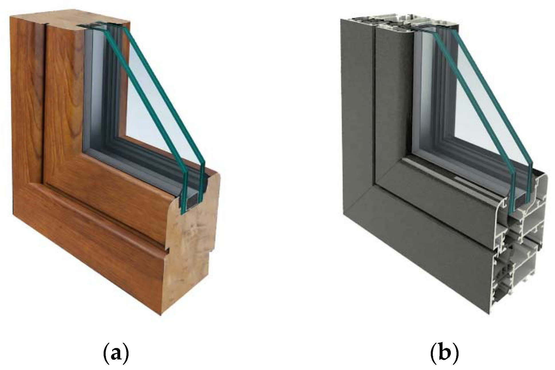
The analysis is conducted on elements with the same energy performance in order to identify the preferable component from a sustainability viewpoint. It is considered the construction phase [39], also taking into account the EE and the EC that the realization implies, in relation to both the service life of the components (in terms of maintenance costs, replacement costs, and so forth) and to the end-of-life phase of the same. Therefore, the focus is not on the energy performances of the components (being assumed equal), but rather on the characteristics of the constructive/executing process, including the environmental impacts in the realization phase (construction) and in the management phase (use–maintenance–adaptation).

Starting from these premises, in order to develop the analysis and calculate the results of Equation (4), the model input definition represents a fundamental phase.

The literature offers consolidated approaches to define the model input. For example, the methodology illustrated in Reference [37] is articulated in the following operative steps:

(1)

identification of each LCCE and, from among these, the selection of the relevant cost drivers (risky or uncertain input cost items);

(2)

for each relevant cost driver, the identification of the potential range of variability to the point estimate;

(3)

calculation of the overall range associated to the estimate, according to two different approaches: the deterministic one (variability range defined according to a minimum and maximum point estimates) and the probabilistic one (variability range expressed through probability distribution functions, calculated with the analytic approach or through simulation).

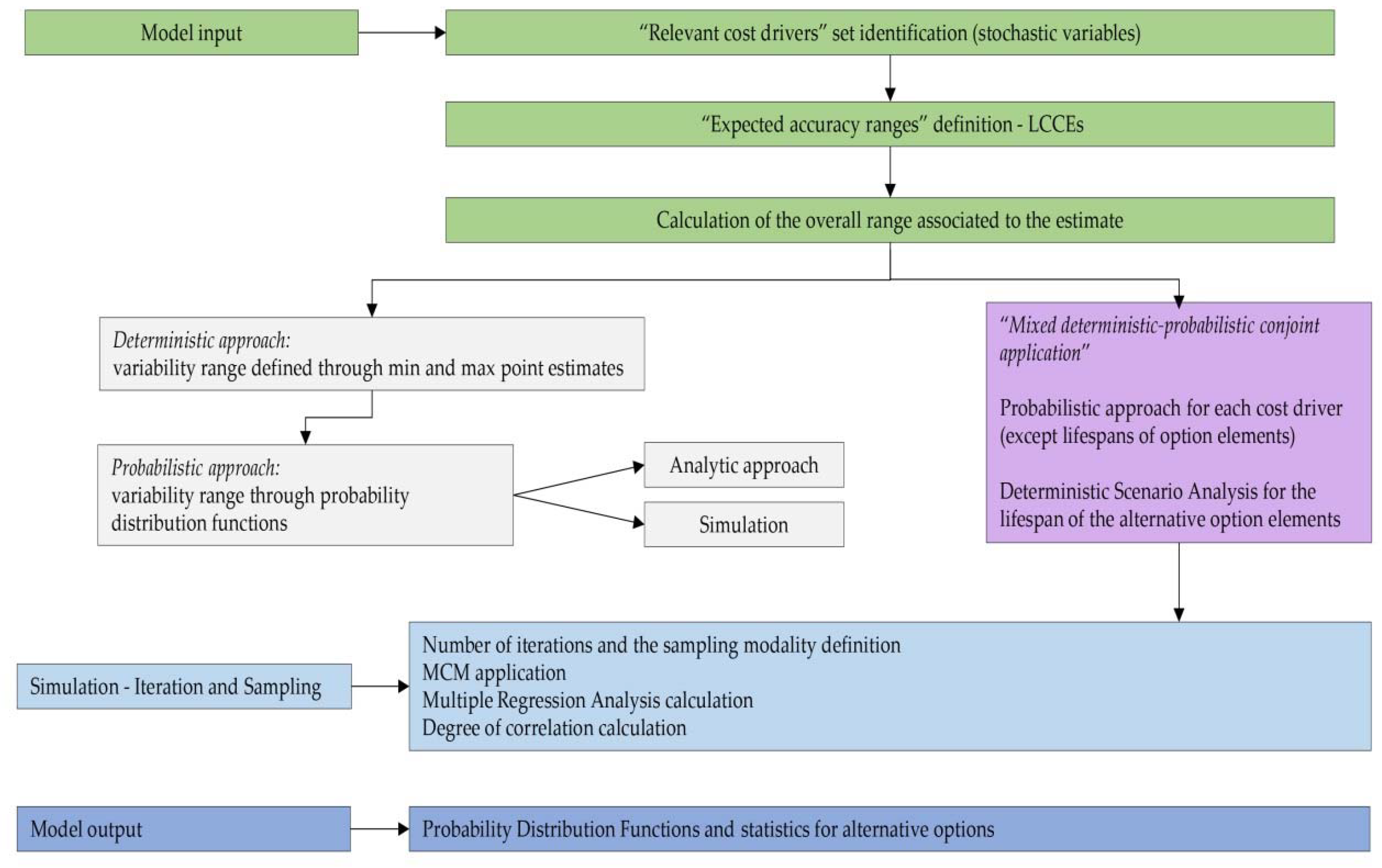
In the application proposed in this work, the input definition phase follows a different workflow. The first two steps are developed in the same modality, while step three is solved through a “mixed deterministic–probabilistic conjoint application”. The probabilistic approach is proposed for defining every variable (cost item), with the exception of the lifespan of the alternative option elements. The latter is modeled according to the deterministic scenario analysis.

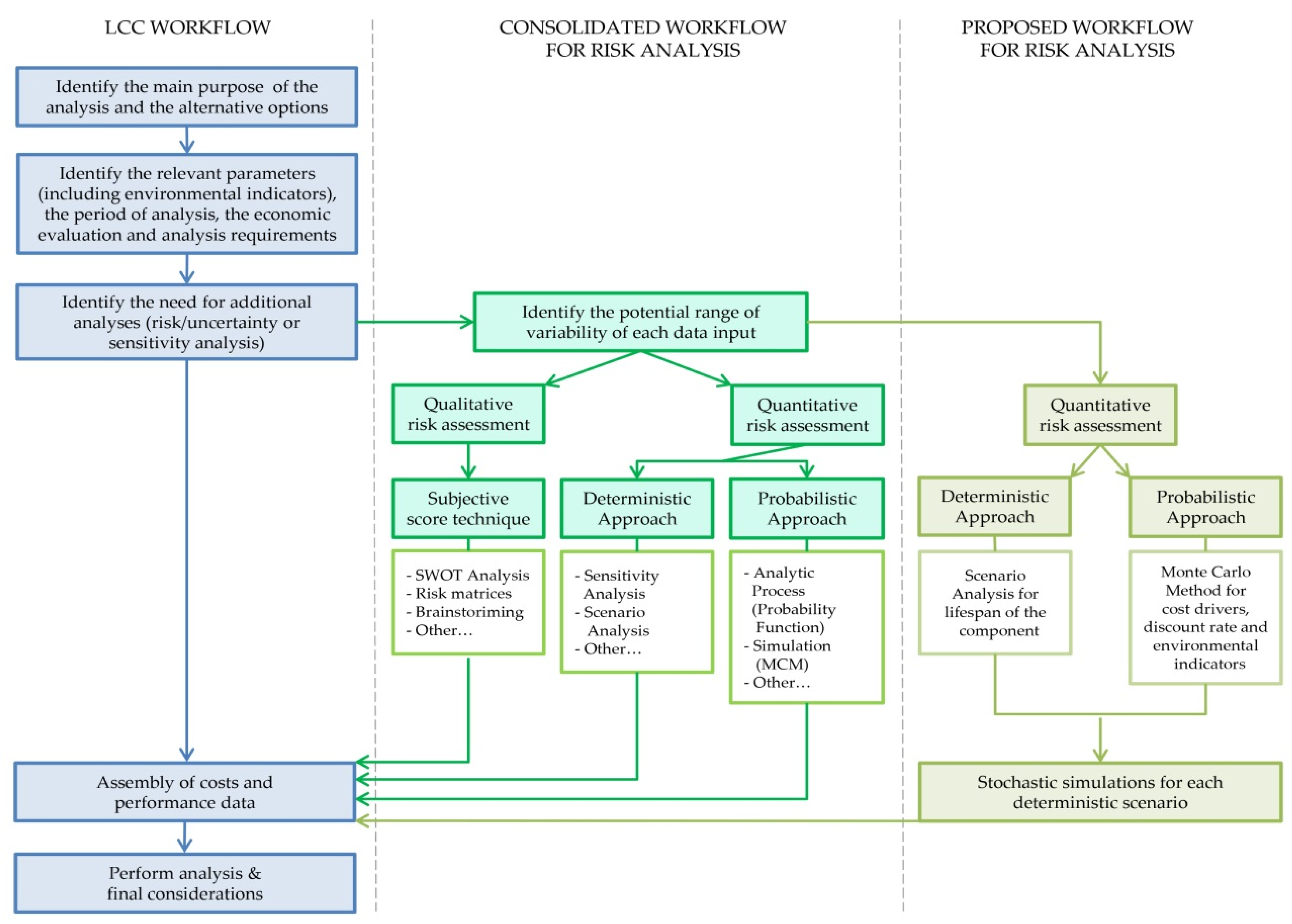
The input definition phase is followed by the model output calculation according to the probability analysis approach. In summary, the methodology is articulated according to the steps illustrated in Scheme 1.

Specifically, the steps illustrated in Scheme 1 are articulated as follows:

• identification of the set of “relevant cost drivers”, or critical inputs, to be expressed as stochastic variables. Costs are subject to different degrees of uncertainty, also in relation to the time. For this reason, it is suggestable to define different confidence levels of the estimates, or “expected accuracy ranges” [37], in relation to the different cost items. Since the costs refer to the life-cycle of the components, the “expected accuracy ranges” can be appropriately expressed in terms of life-cycle cost estimates—LCCEs;
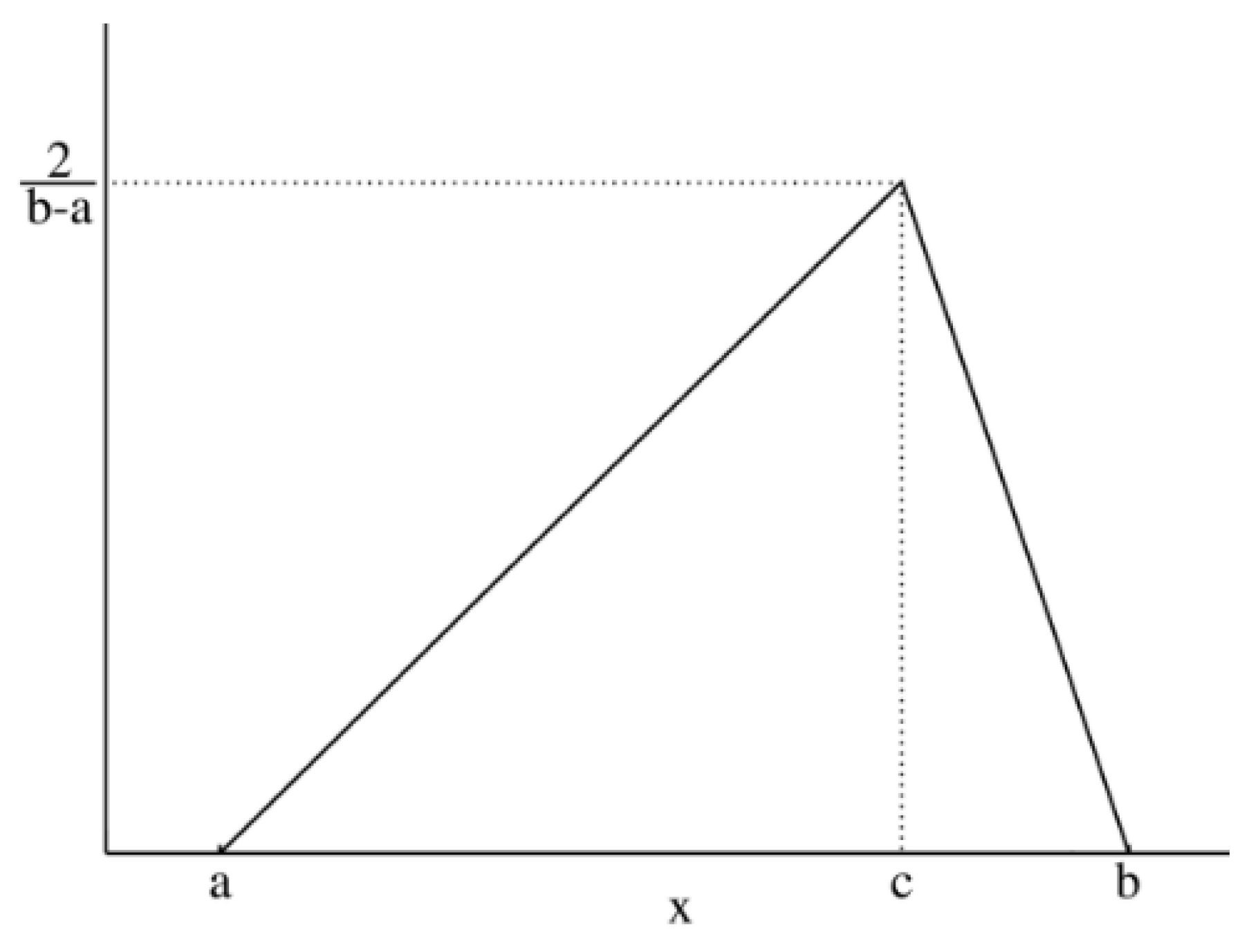
• assignment of the Probability Distribution Function (PDF) to each stochastic input variable, and the identification of the relative probability distribution parameters. As said before, the triangular distribution can be considered the most used PDF to represent the uncertain variables present in the real estate investments (Figure 1) [40,41,42]. Therefore, this step is devoted to the assignment of minimum, maximum, and point estimate values for each variable;
• definition of alternative scenarios with different lifespans in order to simulate different residual values for the components considered in the analysis. In this step, the aim is introducing uncertainty in the duration of the components. The duration is expressed through the variation of the residual values, being uncertain the lifespan of the components themselves;
• Iteration and sampling resolved through MCM. For the simulation, it is necessary to define the number of iterations and the sampling modality, in our case the Latin Hypercube Sampling (LHS);
• running the simulation and production of the regression analysis in order to quantify the effect of the input variables on the output value, expressed in terms of marginal coefficients of the dependent variables against the independent variable (Global Cost). This step is supported by the production of graphics (tornado graphs and spider graphs). Operatively, this step is solved according to the following passages:

  -

  Multiple regression analysis application (usually, sensitivity analysis according to the simulation approach is solved through multiple regression analysis. Formally, the regression model applied for the simulation can be approximated by the following Equation (see Kleijnen, J.P.C., Verification and validation of simulation models, European Journal of Operation Research, 1995, 82, 145–162, p. 156):

  $$y_i={\beta }_0+{\displaystyle \sum }_{k=1}^K{\beta }_k{x}_{ik}+{\displaystyle \sum }_{k=1}^{K-1}{\displaystyle \sum }_{k^{\prime }=k=1}^K{\beta }_{k{k}^{\prime }}{x}_{ik}{x}_{i{k}^{\prime }}+e_i$$

  (5)

  where y_i represents the results of the simulation in the i combination (or run) of the simulation inputs k, for i = 1, …n (where n represents the total number of simulation runs); x_ik stands for the value of the simulation input, k, in the i combination; β_k is the first order effect of input k; β_kk is the interaction between the k and k’ inputs; and e_i stands for the approximation or best-fit error in the i run.) The sampled values of the input variables are regressed against the output variable through multivariate stepwise regression analysis. In LCCA, if the global cost is taken as the dependent variable in the regression equation, then the marginal coefficient calculated for each input variable measures the sensitivity of the output variable with respect to each of them;

  -

  Degree of correlation calculation. This is expressed by coefficients of correlation between the output values and each set of input value samples. Operatively, this step is solved through the rank correlation analysis, calculating Spearman’s correlation coefficients in order to determine the correlation between the global cost and the samples for each input distribution;

• output calculation in terms of the Probability Distribution Functions and statistics (minimum value, maximum value, standard deviation, skewness, kurtosis, and so forth) calculated for each alternative option.

In conclusion, the following summary Scheme 2 shows a comparison between the consolidated procedure [28,37] on the left side and the simplified procedure proposed in this study on the right side. Specifically, the scheme highlights that the sensitivity analysis (according to the deterministic approach), input estimates calculation through probability distributions, Monte Carlo simulation, and analytical techniques, are combined differently in the methodological proposal.

4. Case Study

The methodology proposed is applied for evaluating the preference between two alternative windows realized through different technological solutions. The windows are part of a building project outcome of a design experience considered as a case study in a previous research study [32]. As the present study is the continuation of the previous one, all of the data refers to the year 2015.

The project, which is composed of four independent units, is a multifunctional building with two floors for a shopping mall and the above four floors as an office. It is characterized by a particular shading device that covers the terraces facing the glass façade in the office floors, which was intended to reduce the solar incidence in the summer and optimize the solar gain in winter (Figure 2).

Only one of the four building units is considered, with a gross internal floor area of 4166 m², a total glazing area of 1426 m², and a glazing ratio of the external walls of 90%.

The glass façade is solved through two different technological solutions. In the first case, a timber frame window is adopted; in the second case, an aluminum frame window (see Figure 3) is adopted. Both of them have double selected low-emission glazing filled with argon (4 + 4/12 mm argon 90%/3 + 3). In particular, the two solutions have both the same value of window transmittance (Uw), which is lower than the limit value imposed by the regulations issued in Italy, especially in the force in the City of Turin [43,44].

It is important to notice that even in the presence of the same technological characteristics, according to an economic viewpoint, the timber window system is more expensive (about 30%) than the aluminum one [45,46]. The environmental indicators related to the alternative window systems are carried out with different software tools (see

Table 2. The main economic and environmental indicators of window systems.

Indicator	Unit of Measurement	Timber Frame	Aluminum Frame
Initial investment cost	€	363,027.50	272,852.50
Embodied Energy	MJ	2,333,539.78	5,881,721.38
Embodied Carbon	kg CO2 eq (100 years)	665,485	1,100,860

):

• The IREEA tool (Initial and Recurring Embodied Energy Assessment, Version 2.4, IREEA, Turin, Italy) [47] for Embodied Energy calculation;
• The Designing out Waste Tool (DoWT, WRAP, Banbury, UK) [48] for Embodied Carbon calculation.

The following Table 2 summarizes the main economic and environmental characteristics of the two window systems.

5. Application and Results

According to the methodology illustrated in Section 3, and assuming the case study illustrated in the section above, the following results are obtained.

5.1. Risk and Uncertainty in Model Input

In order to define the uncertainty in LCCEs, firstly, the “critical” input variable or relevant cost drivers are identified. Then, in relation to the potential uncertainty in the estimates, two different ranges are identified in terms of minor (−5% to +10%) and major uncertainty (−10% to +20%).

For each relevant cost driver, an expected accuracy range is fixed, which represents the confidence percentage. As suggested in the literature, the ranges are defined by firstly assuming the opinions expressed “by a group of subject matter experts” [37]. Secondly, the ranges adopted in the risk analysis simulations, the results of recent studies, and the applications for similar items are taken into consideration [49,50].

The cost items and the relative expected accuracy ranges are illustrated in

Table 3. The cost drivers and the relative expected accuracy ranges.

Cost Driver	Expected Accuracy Range
	Low	High
Initial investment costs (elements costs)	−5%	+10%
Annual running and replacement costs:
-  Inspection	−5%	+10%
-  Preemptive maintenance	−5%	+10%
-  Maintenance work (light)	−5%	+10%
-  Maintenance work (main)	−10%	+20%
-  Replacement	−10%	+20%
Dismantling cost	−10%	+20%
Disposal cost	−10%	+20%

.

Notice that the initial investment costs (element costs), dismantling costs, and disposal costs are expressed through the total amount of costs, whilst the others are expressed as yearly or periodic cost amounts according to the components’ lifespans.

Then, the range of values for each cost item both in the case of the timber frame and in the case of the aluminum frame are defined (see

Table 4. The cost drivers and relative probability distribution parameters in the timber frame case.

Timber Frame
Cost Driver	Unit	Low Range	Point Estimate	High Range
Initial investment costs (elements costs)	€/m2	218.06	229.53	252.49
Annual running and replacement costs:
-  Inspection	€ per year	6220.05	6547.43	7202.17
-  Preemptive maintenance	€ per year	15,550.13	16,368.56	18,005.42
-  Maintenance work (light)	€ every 3 years	62,200.54	65,474.25	72,021.68
-  Maintenance work (main)	€ every 7 years	117,853.65	130,948.50	157,138.20
-  Replacement	€	339,561.00	377,290.00	452,748.00
Dismantling cost	€/m2	29.70	33.00	39.60
Disposal cost	€/ton	49.50	55.00	66.00

and

Table 5. The cost drivers and relative probability distribution parameters in the aluminum frame case.

Aluminum Frame
Cost Driver	Unit	Low Range	Point Estimate	High Range
Initial investment costs (elements costs)	€/m2	157.99	166.31	182.94
Annual running and replacement costs:
-  Inspection	€ per year	2253.36	2371.96	2609.16
-  Preemptive maintenance	€ per year	11,266.82	11,859.81	13,045.79
-  Maintenance work (light)	€ every 5 years	45,067.29	47,439.25	52,183.18
-  Maintenance work (main)	€ every 10 years	74,716.82	83,018.69	99,622.00
-  Replacement	€	258,403.50	287,115.00	344,538.00
Dismantling cost	€/m2	29.70	33.00	39.60
Disposal cost	€/ton	−640.00	−800.00	−880.00

). These values, specifically the Low Range value, Point Estimate, and High Range value, represent the distribution parameters that are necessary to define a triangular distribution, as illustrated in the methodology section above.

For the variables of discount rate, Embodied Energy (expressed in terms of the cost for electricity), and Embodied Carbon (expressed through the average value of the carbon taxes applied in the European Member States) [51], the ranges of the values are defined on the basis of specific considerations. Specifically, the discount rate distribution parameters are fixed, assuming the indications of the official documents [28,33]. The Embodied Energy distribution parameters are defined, assuming an expected accuracy range that is coherent with the initial investment costs, and the Embodied Carbon parameters are fixed according to the lowest and the highest carbon tax tariffs (see

Table 6. The financial assumptions and environmental cost items: probability distribution parameters.

Timber/Aluminum Frame
Finacial Assumptions and Environmental Cost Items	Unit	Low Range	Point Estimate	High Range
Discount rate	%	1.25	1.39	2.50
Embodied Energy—Cost for electricity	€/Kwh	0.145	0.153	0.168
Embodied Carbon—Carbon Tax EU	€/ton	13.50	22.25	33.00

).

For the time horizon for the LCCA application, a 30-year lifespan is assumed. Then, in order to consider the residual value of the components as well, three alternative scenarios are assumed, with different lifespan each: 25 years, 20 years, and 15 years. These three alternative lifespan scenarios give origin to three different potential residual values. Consequently, in the 25-year lifespan case, the residual value is defined in relation to 20 years of residual lifespan, and in the 15-year lifespan case, the residual value will be zero.

On the basis of the previous assumptions, a simulation is conducted through the software @Risk (release 7.5 by Palisade Corporation). The simulation is produced through a Monte Carlo Method application, specifically with 100,000 iterations and with a Latin Hypercube Sampling modality.

The probability distributions obtained by processing the input data defined previously are presented in

Table 7. The cost drivers and probability distribution values in the 25-year lifespan scenario; Monte Carlo simulation output.

Cost Driver	Graph	Min	Mean	Max	5%	95%
Disposal cost_glass		72.04174	82.66666	95.9882	75.09819	91.6178
Disposal cost_timber		49.52516	56.83334	65.97852	51.63001	62.98751
Disposal cost_aluminum		640.3812	773.3333	879.7273	683.8148	849.0135
Dismantling cost		29.70633	34.1	39.59618	30.97808	37.7925
Discount rate		1.25%	1.71%	2.50%	1.34%	2.24%
Embodied Energy_cost of electricity		0.1453121	0.1555333	0.1682803	0.1482755	0.1641051
Embodied Carbon_Carbon Tax mean EU		13.51154	22.91667	32.9786	16.42056	29.7623
Fixture Elements Cost:
Fixture elements cost/Timber		218.0984	233.3584	252.466	222.5009	246.2
Fixture elements cost/Aluminum		157.9929	169.0794	182.8887	161.2125	178.3837
Inspection:
Inspection/Timber		6221.259	6656.549	7200.021	6346.84	7022.841
Inspection/Aluminum		2253.682	2411.495	2608.782	2299.294	2544.194
Maintenance Work (Light):
Maintenance work (light)/Timber		62,215.12	66,565.48	71,997.41	63,468.33	70,228.49
Maintenance work (light)/Aluminum		45,079.43	48,229.91	52,172.09	45,985.94	50,883.93
Maintenance Work (Main):
Maintenance work (main)/Timber		117,859.3	135,313.5	157,064.5	122,924.9	149,965.5
Maintenance work (main)/Aluminum		74,738.78	85,785.84	99,568.09	77,931.94	95,074.59
Preemptive Maintenance:
Preemptive aintenance/Timber		15,553.31	16,641.37	18,002.42	15,867.11	17,557.11
Preemptive maintenance/Aluminum		11,269.82	12,057.48	13,043.91	11,496.46	12,720.99
Replacement:
Replacement/Timber		339,753	389,866.3	452,551.2	354,172.4	432,081.8
Replacement/Aluminum		258,436.4	296,685.5	344,450.6	269,523.2	328,811.6

. In the table, the triangular distributions calculated for the 25-year scenario, for each cost element, and the elementary statistics (minimum, maximum, and mean values; 5% and 95% percentiles) are specified.

As illustrated in Table 7, the graphical representation of the probability distributions present, in one case, a triangular distribution with asymmetry on the right. In this case, the outcomes are replaced by incomes, which are represented by the recovery of the aluminum during the disposal phase.

Analogously, the simulations are produced for the 20-year scenario and the 15-year scenario.

5.2. Risk and Uncertainty in Model Output: Stochastic Simulation Through the Monte Carlo Method

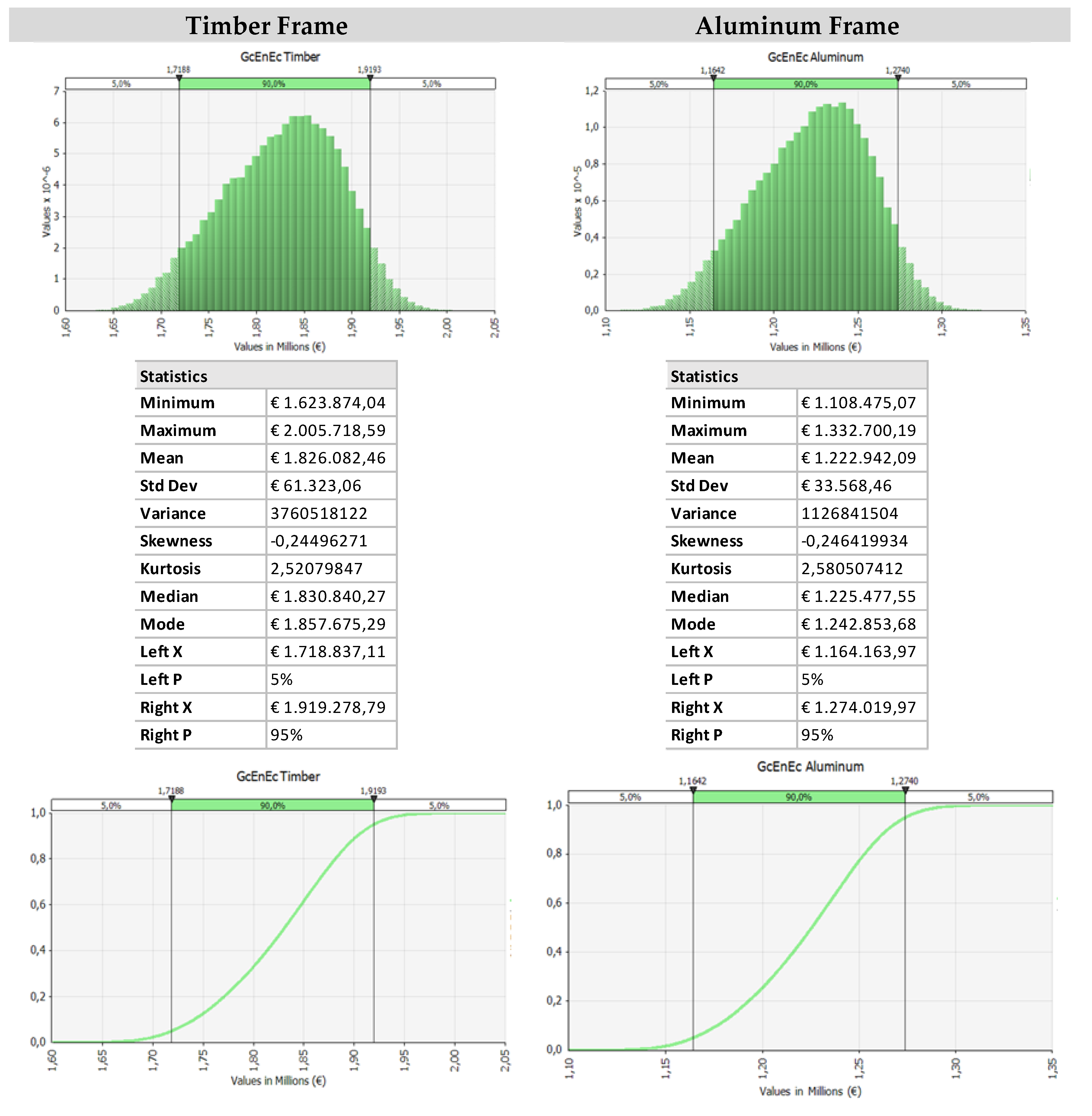
Using the inputs defined in the previous section, the Monte Carlo Method is applied in order to obtain the stochastic output values of the indicator G_CEnEc, as defined in the methodology section.

As illustrated in Figure 4, the first scenario presents the results considering the timber and aluminum frames for a 25-year lifespan. Comparing the probability distribution function of the G_GcEnEc, the related Probability Density Function, and the statistics calculated for the two alternative frames, higher costs emerge for the timber frame, as expected from being in the presence of higher initial and periodic maintenance cost amounts.

In Figure 4, the probability distribution graphics present a similar trend, given the homogeneity of the distribution in the input data. The differences are present in the minimum, mean, maximum values, and in the standard deviation values.

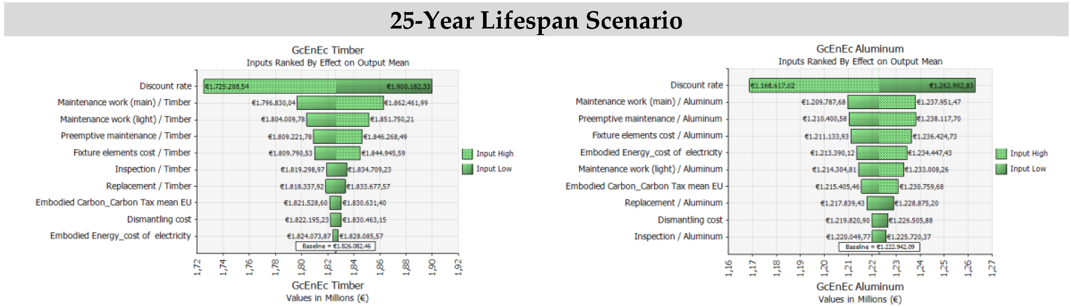
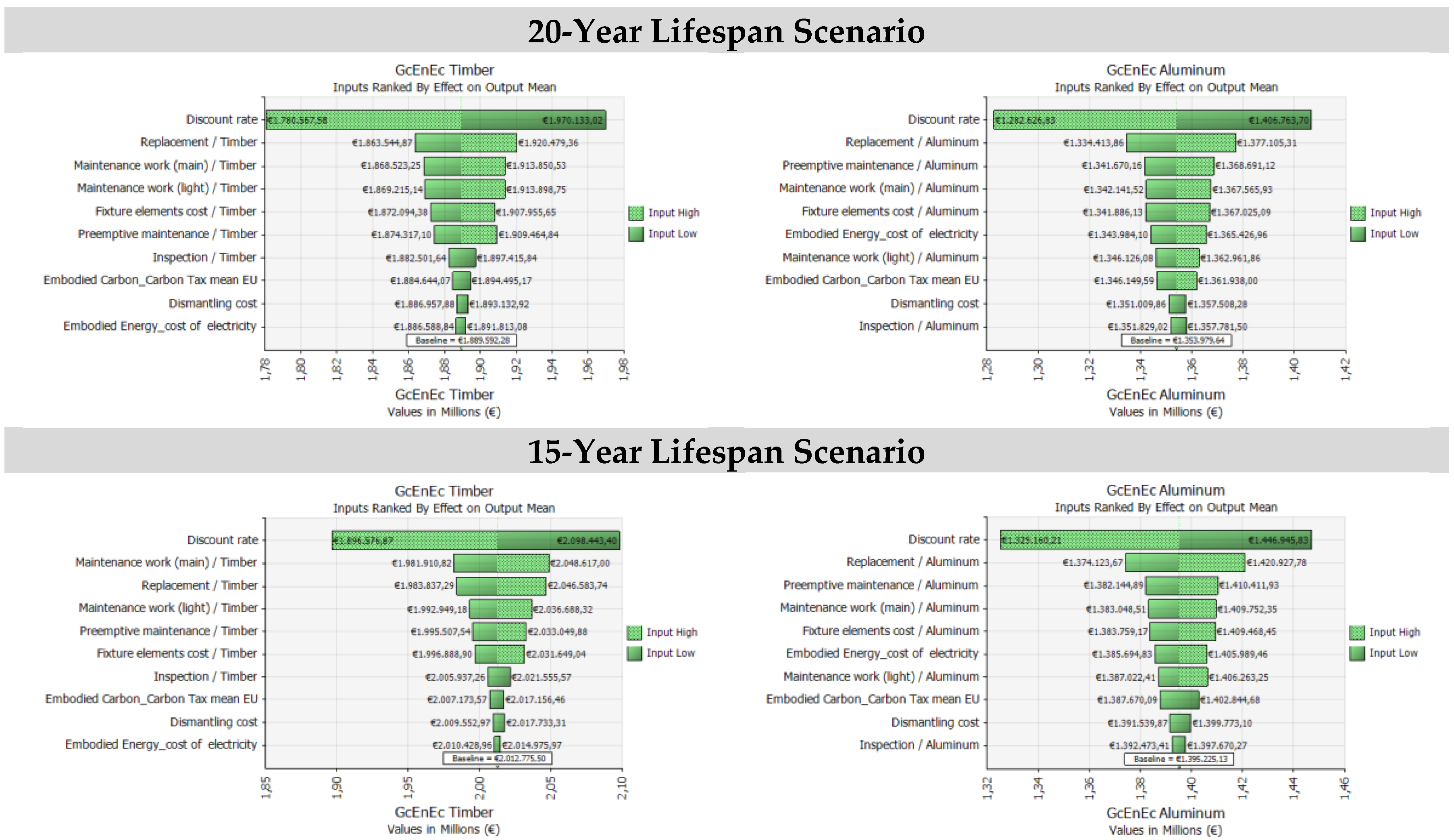
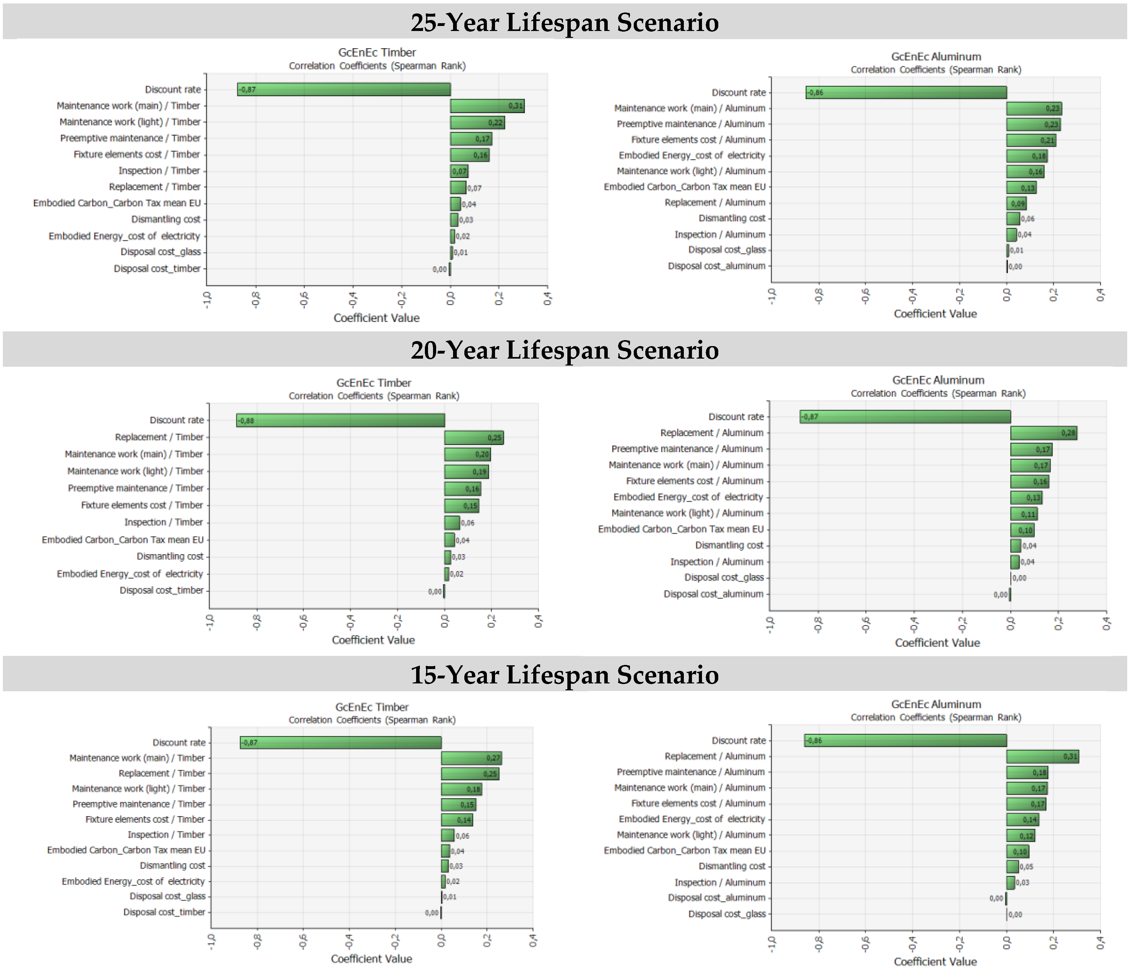
Analogously, the simulations are produced for the 20-year and 15-year scenarios, considering both timber and aluminum frames. The results of the simulations are synthetically reported in Figure 5 and Figure 6, in which the tornado graphs related to the effects of the inputs on the output mean and related to the Spearman correlation coefficients to determine the correlation between the global cost and the samples for each input distribution are illustrated.

Comparing the results of the regression analysis application, graphically represented through a tornado graph (see Figure 5 and Figure 6), the following considerations emerge:

• for every scenario, the discount rate is the variable that produces the largest perturbation on the output. In fact, considering the range of values assumed for this variable, the effects on the output are relevant;
• cost items regarding preemptive maintenance, light maintenance work, and the main and elements costs are relatively significant, while the other items have a small influence on the results;
• the relative influence of Embodied Energy is particularly significant in differentiating the aluminum frame and the timber frame;
• the substantial effect of the residual value and the related uncertainty on components lifespans in differentiating the output results in favor of the aluminum frame technological solution.

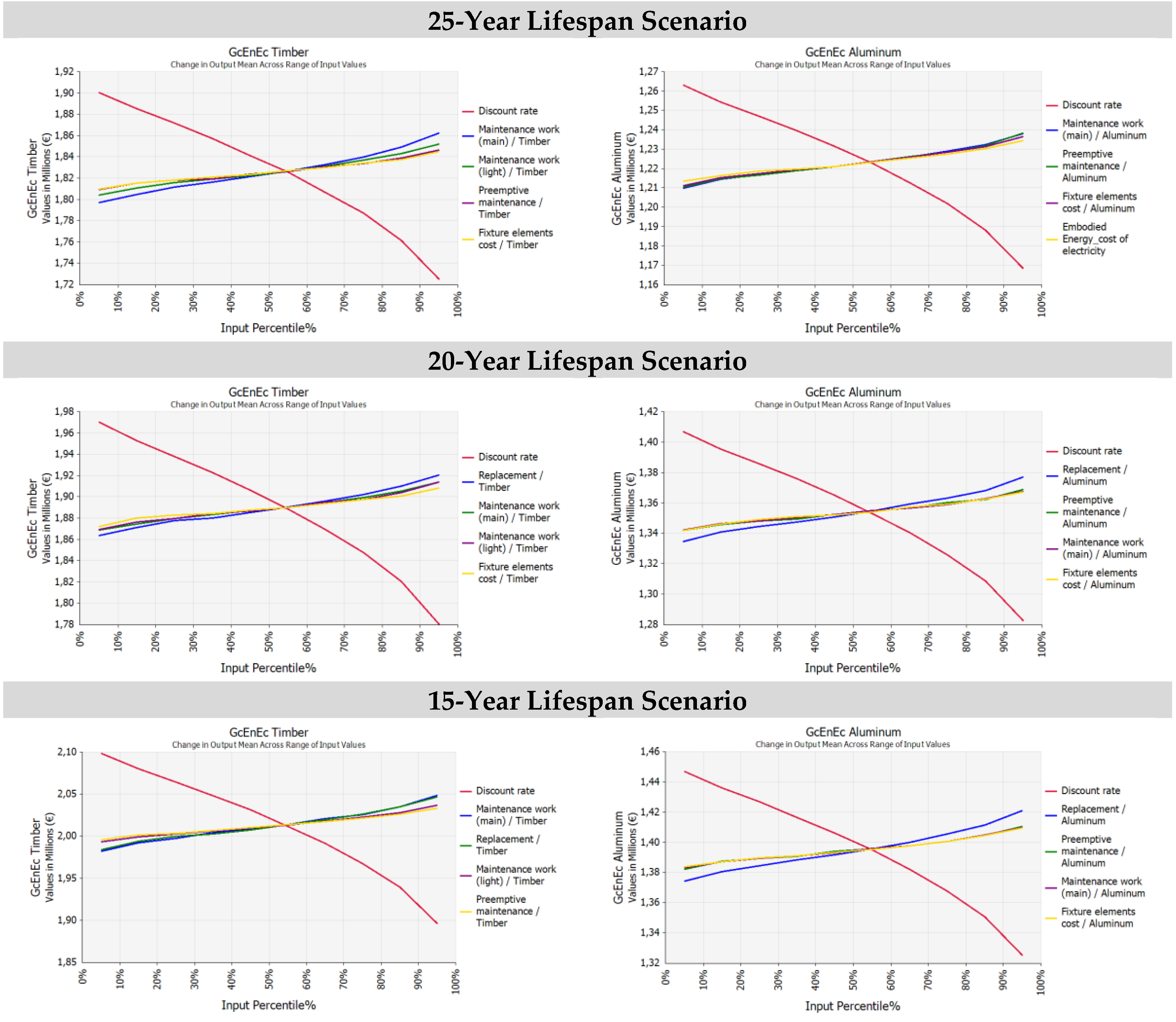
These considerations are supported also by the analysis of the spider graphs (see Figure 7).

The spider graphs confirm the relevant effect of the discount rate (red line) with a negative trend, whilst the results of the other lines (with positive trends) are rather overlapped in every case with a limited difference.

5.3. Results and Final Considerations

Concluding the analysis, the simulation output results are compared as reported in

Table 8. The output values of Gc_EnEc for the timber/aluminum frames: the probability distribution function and statistics for the 25-year lifespan option. The Monte Carlo simulation output.

Output	Graph	Min	Mean	Max	5%	95%
GcEnEc Timber		€1,623,874.00	€1,826,083.00	€2,005,719.00	€1,718,837.00	€1,919,279.00
GcEnEc Aluminum		€1,108,475.00	€1,222,942.00	€1,332,700.00	€1,164,164.00	€1,274,020.00

,

Table 9. The output values of Gc_EnEc for the timber/aluminum frames: the probability distribution function and statistics for the 20-year lifespan option. The Monte Carlo simulation output.

Output	Graph	Min	Mean	Max	5%	95%
GcEnEc Timber		€1,664,037.00	€1,889,592.00	€2,093,332.00	€1,774,911.00	€1,988,238.00
GcEnEc Aluminum		€1,210,552.00	€1,353,980.00	€1,492,126.00	€1,278,157.00	€1,419,990.00

and

Table 10. The output values of Gc_EnEc for the timber/aluminum Frames: the probability distribution function and statistics for the 15-year lifespan option. The Monte Carlo simulation output.

Output	Graph	Min	Mean	Max	5%	95%
GcEnEc Timber		€1,768,091.00	€2,012,776.00	€2,250,914.00	€1,889,712.00	€2,119,987.00
GcEnEc Aluminum		€1,232,633.00	€1,395,225.00	€1,547,834.00	€1,320,232.00	€1,461,350.00

, respectively, for the 25, 20, and 15-year lifespans.

From the results, it is also possible to extrapolate the effect of the residual value.

In contrast with the considerations about the environmental impacts of the two different scenarios, the aluminum frame seems preferable under the economic viewpoint.

In fact, the residual value assumes a higher significance in the case of timber, while for aluminum, the effect in terms of the global cost is lower or more stable. In the case of a lower or absent residual value for timber frame, the global cost increases considerably: timber seems more reactive to the residual value reduction, as the timber component is more expensive. On the contrary, the aluminum component scenario seems less reactive to residual value variations.

These last considerations open up the opportunity to analyze deeply the behavior of the two technologies from a time perspective, in terms of the uncertainty over time, or, in other words, the necessity to analyze the residual value as a function of time by introducing stochastic processes into the analysis.

6. Conclusions

In this paper, a methodology aimed at supporting decision making in new buildings or in retrofitting design activities was proposed. The method assumed a life-cycle perspective and sustainable design principles [52]. The focus was on the evaluation of the economic–environmental sustainability, considering the presence of the risk and uncertainty components. The presence of uncertainty in both cost-estimating (LCCEs) and in technical performance (LCCA) was particularly assumed.

With these purposes, an application of the Life-Cycle Cost Analysis in conjunction with a risk analysis was proposed to select the preferred choice from among the alternative technological options, taking into account both the economic and environmental aspects.

Specifically, the risk analysis was solved through the probability analysis approach, which was developed by the following steps: (1) identification of the set of “relevant cost drivers” expressed as stochastic input variables and the definition of the relative expected accuracy ranges; (2) the assignment of the probability distribution function (triangular distribution) to each stochastic input variable and the identification of the relative probability distribution parameters; (3) the definition of alternative scenarios with different lifespans in order to simulate different residual values for introducing uncertainty in the duration of the components; (4) iteration and sampling through the Monte Carlo Method; (5) the running of the simulation and the production of regression analysis; and (6) output calculation for each alternative option.

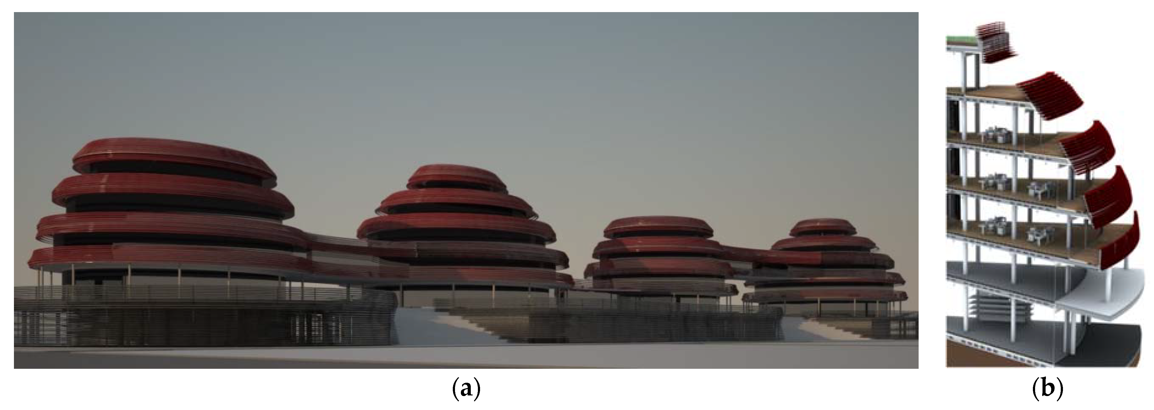
The methodology was applied on a simulated case study regarding the selection of the preferable solution from between two alternative technological components, in economic and environmental terms, for a multifunctional building glass façade in Northern Italy. The same case-study was treated in a previous work of which this paper constitutes a development.

Coherently, with this previous study, the evaluation of the sustainability of the project, both in economic and environmental terms, is analyzed with a synthetic “economic–environmental indicator”, calculated in terms of a stochastic global cost.

Considering the results of the regression analyses produced, it emerged that the uncertainty in the discount rate input variable can determine the largest perturbation on the output, confirming the relevance of financial variables in long-term valuations such as LCCA applications. Contrarily, cost items are relatively or poorly significant in the results. Meanwhile, the relative influence of environmental variables is particularly significant in differentiating the aluminum frame and the timber frame. The presences of EE and EC are able to perturb the model output and lead to opposite results, with respect to the deterministic model application. Furthermore, the substantial effect of the residual value and the related uncertainty on components’ lifespans in differentiating the output results in favor of the aluminum frame technological solution was observed.

The behavior of the two technological scenarios under uncertain conditions opens the necessity of developing a further step of the analysis that considers the influence of time (duration of components) as a stochastic variable. The progress of the research is directed to the exploration of stochastic processes in order to model the variation of economic impacts, assuming flexibility in the input data and in service lives.