Smoking Gentlemen—How Formula One Has Controlled CO₂ Emissions

Abstract

This article reports estimates of the level of CO₂ emissions created by Formula One (F1) cars on Sunday races. Supported by a variety of sources and using Monte Carlo iterations, we obtained values identifying important periods of change. These periods were identified using tests of structural breaks. We observe that the 1966–1970 period (related to the dominance of DFV/Cosworth engines) is associated with an increase in CO₂ emissions, whereas the 1992–1995 period (related to lighter and more efficient engines) is associated with a decrease in estimated levels of emitted CO₂. Our results do not identify the deep modifications following more “green” regulations in 2009–2011 as a relevant change.

1. Introduction

CO₂ emissions are currently a generalized concern for most citizens. Environmental issues are also found at the top of citizens’ priorities, as revealed in recently divulged surveys. Several sources of CO₂ emissions exist, of which “transportation” activities are not a negligible group. Several works have recently contributed to highlight the relevance of this topic. We are particularly thinking about the works of Fulton et al. [1] or of Centobelli et al. [2], who provided a proper salience for the environmental requirements established by the five main climate change agreements: in 1992, the United Nations Framework Convention on Climate Change; in 1998, the Kyoto Protocol; in 2009, the Copenhagen Accord; in 2012, the Doha Amendment; and in 2015 the Paris Agreement. It is undeniable these agreements have generated significant stimuli in transportation industry and in motorsports.

Most “transportation” activities are related to the daily use of cars, ships, or planes. However, given their proximity and frequent use by most citizens, car emissions are particularly analyzed in the literature.

Although most attention on the linkage between CO₂ emissions and the automobile sector are put on the daily activities of individuals and firms, motorsports also have a certain responsibility for the total volume of CO₂ emissions by vehicles. There are several reasons behind the importance of motorsports on CO₂ emissions that are explored in this paper. Some of these reasons relate to the “direct effects” of the type of combustible engine used in various motorsports, the high effort/work of the competing engines, as well as the “indirect effects” coming from the additional transportation of the teams, engines, chassis, and fans/spectators to the venues.

Within motorsports, Formula One (F1) has responsibilities concerning this topic. Being one of the most expensive sports, with a high level of consumption of fuel by each engine and with a significant number of regular races per season, Formula One can be considered a regular source of CO₂ emissions for the last seven decades in the world of motorsport.

However, until now, there has not been a robust attempt to estimate the CO₂ emissions per race since 1950. This kind of estimation would provide a value for the costs of these emissions and, more importantly, would enable the analysis of the evolution of these emissions since the first race organized by the FIA (Federation Internationale de l’Automobile)—the Silverstone/1950—until the present.

Therefore, in this paper, we propose the estimation and analysis of the values of CO₂ emissions by F1 races and by F1 seasons since the Silverstone/1950. As a consequence, this manuscript contains challenging contributions to the new body of knowledge. Taking into consideration the different types of engines used in F1 cars for each season, the number of cars per race, and the length of each race run by each competing engine, we had the basis for estimating the values of CO₂ emissions in Formula One races.

We collected data for the F1 cars’ tank capacity. We also took in consideration the number of cars which started in the races. Then, we observed the complete number of laps of each car. After this step, using Monte Carlo iterations, there was the estimation of the number of consumed liters of fuel per race and the level of CO₂ corresponding to the estimated value of consumed liters.

For each of these series, we studied the stationarity profile and the related structural breaks using a framework from the Time Series Analysis. The results of the tests on structural breaks identified the period of the dominance of the turbochargers and Cosworth engines as a period of higher CO₂ emissions. The 5-year period after 1992, characterized by different engines, had been associated to a period of decreased emissions. There were deep modifications towards a more ecologically maintainable sport in Formula One’s regulations in the recent 2009–2011 period. However, our empirical achievements did not detect a significant change in the global level of CO₂ emitted by F1 cars during Sunday races after this 2009–2011 period.

The remainder of this paper is organized as follows. Section 2 reviews the literature on motorsports and on Formula One as sources of CO₂ emissions. Section 3 details the empirical exercise done to estimate the values of CO₂ emitted in each F1 race (majorly detailing the Sunday events and considering emissions from F1 cars). Using Monte Carlo simulations and analyzing structural breaks estimated for the series of tank capacity, the number of starting cars, the percentage of laps raced, the liters of fuel consumed per race, and the estimated emissions of CO₂, additional evidence found is discussed. Section 4 concludes the paper, presenting challenges for further research and for policy implications.

2. Review of Literature—CO₂, Motorsports, and Formula One

2.1. Motorsports as a Source of CO₂

The literature widely identifies an uptrend in citizens’ concerns about the complexity of pollution sources worldwide [3,4,5]. Besides citizen concerns, there is evidence of more intense political activity on the topic, independent of national parliaments and governments [6,7] or the international space of multilateral agreements [8,9].

The volume of pollution related to a place, period, source, or flow is discussed using a kind of “common denominator”: the intensity of CO₂—i.e., carbon dioxide emissions [10]. Following Steen [11] or Ahmad et al. [10], the largest contribution to the greenhouse effect also stems from emissions of carbon dioxide. The same source [11] points out that “75% of the global CO₂ emissions result from the combustion of fossil fuels for the transformation and use of energy.”

The sources of CO₂ emissions are complex. Currently, we know that jargons like “carbon neutral” are not achievable in accurate terms because as soon as we breathe, we generate CO₂ [12]. Therefore, the direction of the ecological suggestions has been in the sense that various sources (daily routines, industrial activities, farming or livestock, etc.) must generate less CO₂ and must continue to improve the quality and the quantity of output (the meaning of “energetic efficiency”, according to Gillingham et al. [13]).

One important source of CO₂ emissions is transportation activities. These activities include a wide range of actions, from the daily use of private and public vehicles transporting passengers, to commercial flights and maritime routes [14,15]. Works like OECD/IEA [16] found that transportation activities create about 23–27% of CO₂ emissions from fuel combustion worldwide.

Road activities have gained attention within the discussion concerning transports/transportation as sources of CO₂ emissions [17,18]. As OECD/IEA [16] suggests, there has been a 71% increase of CO₂ emissions from the road sector since 1990, which accounted for three-quarters of transport emissions in 2014. Figure 1 (extracted from OECD/IEA [16] p. 38) shows this uptrend for most CO₂ sources.

There are relevant surveys about the recent trends that the literature has observed in these scientific fields. Falco et al. [19] provide a robust review about the literature on climate change and extractive activities. Falco et al. [19] highlighted that the importance of agriculture emerges from micro-level country studies and some macro-level analyses using cross-sectional data over longer time periods. Nichols et al. [20] majorly focused the interlinkages between climate changes and sustainability in a different work of literature survey. Nichols et al. [20] identified published literature on health, climate change, and sustainability, and they classified the publications according to their focus on effects, strategy, and actions by additionally providing a thematic analysis of the papers’ content. Finally, Broto and Bulkeley [21] have reviewed the literature focused on urban climate changes. Their analysis suggests that, since 2005, experimentation is a feature of urban responses to climate change across different world regions and multiple sectors.

Correlated with consideration to the road sector, there is growing attention on motorsports [22]. There are two major reasons for this rising concern. The first relates to public awareness of global warming, which has introduced relevant challenges to all motorsports [23,24]. Nick Nuttall (in Allen [25]) of the UN Environment Program claimed, “Motor sports will not be immune to some of the profound sea of changes at work around the globe, from environmental to reputational risk.” The second reason relates to the generalized concern of the accentuated short supply of fossil fuels, even if only considering a medium-term perspective (around the next 50 years).

In terms of carbon analysis, motorsport is a joint space of two dimensions when discussing carbon footprint—its capacity of attracting many people to the venues and the direct sources of pollution derived after the tests, qualifying sessions, and races in regular seasons.

On one side, as with any sport, we can discuss the ecological impact associated with the externalities of matches/races, such as the spectators using fuel to get to the event and back home again over the course of a regular season. Still, in this perspective, the power used by people watching the sports events on television was found to significantly contribute to these values [26,27]. On the other side, it is not hard to identify a complex set of sources of CO₂ emissions related to motorsports, like the fuel combustion in the engines, the research and development activities, or the residuals treatment.

2.2. Formula One as a Regular Source of CO₂ Emissions

Within motorsports, Formula One is widely considered the pinnacle because of its cost, drivers’ payments, prize money, audiences, and world coverage. However, Formula One did not have a good reputation among ecologists until 2010. According to Ornstein [28], Formula One was “probably the most polluting sport on the planet”. Justification for this opinion includes the cars’ internal combustion engines, which are considered one of the most damaging inventions of the planet (Allen [25]), and concerns related to the regular weekends of the competition in which F1 cars, staff vehicles, flights, and other transportation tools cross the globe, generating CO₂ emissions estimated at values higher than 54 tons of CO₂ per driver/car in 2007. Estimates from 2007 also recognize that each car is responsible for about 8.5 tonnes of CO₂ per season (Ornstein [29]). These values led Purcell [30] to qualify F1 as “the antithesis of eco-credibility”. However, the Trucost Report [31] evaluated that only 0.3% of F1′s emissions come from racing and testing the F1 cars (in the Trucost Report [31], it has been found that the two biggest contributors to F1′s “carbon footprint” were the production and supply of raw materials and parts for the team, which accounted for about half the footprint, and from electricity used to power computers, wind tunnels, and the like (30% of the pollutants)).

Since 2009, F1 teams have been engaged in a “race to Green”, enhancing several programs for reducing CO₂ emissions (“We are in F1 because we believe it’s not only a competition among the best drivers in the world, it’s also a competition among the best engineers in the world,” says Toto Wolff, Mercedes head of motorsport (Allen [25])). The most revealing action is related to the in-race refueling ban. However, other measures have also been taken (Galvin [32]).

One important race strategy, with relevant changes in the regulated direction, is refueling. Officially, the first driver adopting such a strategy was Juan Manuel Fangio, during the 1957 German Grand Prix (which he won). However, it was not until the 1980s that the refueling strategy came with a generalized importance in the grid, with the pioneering role of the Brabham team in the Austrian Grand Prix of 1982. The topic was given such priority that FISA—the organizing body of the competition at the time—decided to ban refueling in 1984. The fuel volume permitted for racing was then reduced from 250 L to 220 L (a further reduction to 195 L was made in 1985). However, 10 years later—in 1994—the governing body (FIA) again permitted refueling, making pit stops a crucial part of the winning strategy of a race. During this period, which lasted until 2010, refueling (the average rate of refueling has been estimated as 11 L per second in an F1 car [33]) was only permitted in team garages/FIA garages. Following these regulations, teams could change fuel load during any practice session and during qualify sessions, except during qualifying session 3 and those following. Fuel left after qualifications should be used for the race. Refueling was allowed during the race. If the race was suspended, refueling was strictly forbidden. Amounts of fuel carried by the cars in the first qualifying period had to consider the fuel needs for the next qualifying moments and for the entirety of Sunday’s race. After 2010, with the ban on refueling, teams did not want to carry any more fuel than absolutely necessary to keep the weight of the car to a minimum.

In terms of fuel consumption per race and per engine, the changes in refueling were not null. Cars had to change chassis and fuel tanks in order to optimize the fuel strategy, and systems of fuel cooling were adopted after the ban of 1984. The search for the efficiency of engines became more impetuous [32], trying to increase ratios like “mile per gallon” or liters per hundred kilometers. As Wlock and Bentley [34] stated, important changes were done in the wings and tires in order to reduce fuel consumption. According to Ingram [33], “From 2014, all teams [would] use a 1.6-L turbocharged V-6 engine”, able to produce close to 550 horsepower and a spin of 15,000 rpm. These values reveal a long evolution towards more efficient F1 engines, which shrunk engines from the 4.5 L engines of the Talbot L6 (in the first seasons of 1950s) to the typical 3.5 L engines of the mid-1990s.

However, as we noticed, F1 teams also became deeply engaged in changes toward sustainability, especially after the Trucost Report [31]. For instance, since 2011, McLaren has implemented a number of technologies, namely, programming its factory’s air-conditioning system to only function in areas where staff are currently working, as well as developing a new type of low-energy lamp to illuminate car parks and access roads. Each vehicle in the McLaren fleet is fitted with a monitoring device to gather information on driving efficiency. This data is then analyzed back at McLaren HQ and used to support the training of crew to drive more efficiently (Purcell [30]). As of 2014, F1 cars are powered by 1.6 L hybrid turbo engines, replacing the old 2.4 L V8, which consumed significantly more gas (Mack et al. [34]). These power units comprise an electrical energy storage system capable of injecting 160 horsepower for 33 s. Technically, these cars use about a third less fuel to cover the same distance at the same speed, anticipating new limits in the regulations: instead of 150 kg, the limit will be 100 kg. This change is estimated to reduce the level of CO₂ emitted per kilometer by about 35%. Additional systems of energy recovery are built into each engine (better known as “Thermal Energy Recovery System” or TERS. (TERS is a derivative of an original generation of recovery systems, known as kinetic energy recovery systems, or KERS. According to Edmondson [35], the use of TERS by the winning engine of the 2014 season—the Mercedes’ class-leading hybrid F1—“exceeded 45 percent (…). By contrast, coal and oil power stations achieve thermal efficiency of around 33 percent, meaning the power used to drive an electric car is likely to come from a less efficient source than an F1 engine.”) These systems are expected to be produced in mass numbers for daily use vehicles, intending to save fuel consumption in the near future. There are also various ongoing projects, like building a fuel consumption reducer into the regulatory roadmap, which will require the teams to deliver competitive racing with less fuel.

2.3. F1 Tanks, Fuel Consumption, and CO₂ Emissions

The gas emissions of any engine are mainly due to fuel combustion. There are other CO₂ leaks in a car, although their importance is significantly lower than fuel combustion [33,34]. The regulations in Formula One detail the properties of fuel tanks, as well as the elements associated with fitting, piping, crushable structure, fillers, refueling, and fuel sampling (Wright [36]). The fuel tank must be a single rubber bladder. Following Wright [36] or Fagnan [37], the fuel tank is located in the center of the car, away from the brakes and the engine. The rules stipulate that the fuel tank must be located between the driver’s seat and the engine, and it must not exceed the width of the chassis. The bladder is flexible and must fit the profile of the monocoque. The bladder weighs only 5% of the total mass of fuel it can hold. It is made from puncture-proof Kevlar, which reduces the risk of fire. Usually, the fuel tank (different among F1 teams) is the biggest, single part of the car, representing only 1% of its total weight. Due to the strict rules on fueling/refueling in F1 history, each car’s tank provides an estimation of the liters of fuel expected to be consumed in a race, especially for Sunday events.

Another important element in the discussion focuses on the CO₂ emissions of F1 cars related to the fuel. Fuel (in this case, gasoline) is identified with the liquid that is mixed with air in the cylinder to generate combustion and, therefore, a powerful expansion in the cylinder. The better the fuel is distributed in the combustion chamber, and the more explosive particles there are per cubic centimeter (cc) in the fuel, the more power (usually measured in horsepower) that will be produced with a constant amount of fuel. Currently, the differences between the fuel used by different teams is not as notorious as in the past [35,38,39]. However, the enhancement of fuel properties is always a concern for team strategy.

Fuel is crucial for a keyword in motorsports: efficiency. A car’s efficiency can be improved by lowering fuel consumption while generating the same performance. De Groote [40] declared that “For most of the teams, these fuels are supplied for free by a technical partner that is usually a worldwide manufacturer.”

In the early seasons of Formula One, De Groote [40] noted that “[teams’ engineers] brewed aggressive mixtures from substances such as benzene, methanol, acetone and nitrobenzene, some of which had to be drained from the engine immediately after practice and races. Without this precaution, the engine would not have survived the night. Later on, kerosene was used until the late 1960s, before the list of admissible additives was increasingly narrowed by the sport’s governing body, the FIA, for the protection of drivers and mechanics.” By the 1970s and the 1980s, regulations allowed the use of high-octane gasoline (RON 101 or RON 102), commercially traded in countries like France, Italy, or Germany. The early 1990s seasons witnessed the appearance of new restraints on the properties of admitted fuel in Formula One, as well as experiments with steam pressure, density, benzene, and lead content.

Since 1996, the FIA has used unleaded fuel. By 2001, fuel saving met with 2005 standards approved by FIA. Biofuel (“ethanol”) has also been introduced to lower carbon emissions [41,42]. According to current regulations, F1 fuel must have the same components as consumer fuel. However, the composition/proportion of saturated hydrocarbons (paraffin and naphthenic) and non-saturated hydrocarbons (benzene, toluene, xylenes, diolefins, and acetylene) in F1 fuel is different than the composition of consumer fuel. F1 fuel has a higher proportion of non-saturated (30% compared to 10% in consumer fuel) and a lower proportion of naphthenics (5% compared to 30%).

It is common to use coefficients to determine an estimate of CO₂ emissions by type of fuel. There are various works that present the Carbon Dioxide Emissions Coefficients by Fuel [43]. Common gasoline has an estimated coefficient of 8.89 kg of CO₂ per gallon or 2.349 kg of CO₂ per liter. There are factors exhibiting lower emissions, like propane (5.76 kg of CO₂ per gallon), butane (6.71 kg of CO₂ per gallon), ethanol (7.734 kg of CO₂ per gallon), or even aviation gas (8.35 kg per gallon). However, factors like kerosene (9.75 kg of CO₂ per gallon), home heating and diesel fuel (10.16 kg of CO₂ per gallon), or jet fuel (9.57 kg of CO₂ per gallon) have clearly higher CO₂ emission values. According to Atlas F1 [44], “Mercedes [at 1957], for example, relied on the following recipe: 45% benzene, 25% methyl alcohol, 23% aviation fuel, 3% acetone and 2% nitrobenzene. The remaining two percent remain a secret until this day. The explosive mixture was so aggressive that remnants left over from training and races had to be drained off and the engine rinsed out with conventional petrol. This was the only way to prevent the engine from suffering damage overnight!”

Table 1. Some engines representing the heterogeneity of each decade.

Seasons	Tanks’ Capacity	Displacement/Power
1950–1959	Alfa Romeo 159/1951 (300 L) Lancia D50/1954 (205 L) Ferrari 801/1958 (200 L)	Alfa Romeo 159/1951 (1479 cc, 425 hp@9300 rpm). Lancia D50/1954 (2489 cc, 260 hp@8200 rpm). Ferrari 801/1958 (2486 cc, 285 hp@8800 rpm).
1960–1969	Cooper T51/1960 (150 L) Ferrari 312/1966 (158 L) BRM P138/1968 (173 L)	Cooper T51/1960 (2462 cc, 236 hp@6750 rpm) Ferrari 312/1966 (2989 cc, 390 hp@10,000 rpm) BRM P138/1968 (2998 cc, 390 hp@9500 rpm)
1970–1979	March 711/1971 (272 L) Ferrari 312T/1975 (200 L) Renault RS01T/1977 (200 L)	March 711/1971 (2993 cc, 480 hp@10,600 rpm) Ferrari 312T/1975 (2991 cc, 495 hp@12,200 rpm) Renault RS01T/1977 (1492 cc, 530 hp@10,000 rpm)
1980–1989	ATS D7/1984 (220 L) Williams FW10/1985 (220 L) McLaren MP4/1987 (197 L)	ATS D7/1984 (1500 cc, 850 hp@10,500 rpm) Williams FW10/1985 (1500 cc, 800 hp@11,000 rpm) McLaren MP4/1987 (1496 cc, 850 hp@12,000 rpm)
1990–1999	Williams FW14/1991 (220 L) Tyrrell 024/1996 (120 L) Benetton B198/1998 (125 L)	Williams FW14/1991 (3493 cc, 700 hp@12,500 rpm) Tyrrell 024/1996 (3000 cc, 690 hp@13,800 rpm) Benetton B198/1998 (3000 cc, 750 hp@14,000 rpm)
2000–2009	Sauber C22/2003 (146 L) Renault RS23/2003 (150 L) Honda RA106/2006 (150 L)	Sauber C22/2003 (2997 cc, 855 hp@18,600 rpm) Renault RS23/2003 (3000 cc, 800 hp@18,000 rpm) Honda RA106/2006 (2398 cc, 650 hp@19,500 rpm)
2010–2015	Ferrari 150/2011 (220 L) Ferrari F14/2014 (140 L)	Ferrari 150/2011 (2398 cc, 785 hp@18,000 rpm) Ferrari F14/2014 (1600 cc, 670 hp@15,000 rpm)

Legend: cc, cubic centimeter; hp, horsepower; rpm, revolutions per minute.

introduces some remarkable Formula One engines by their particular characteristics of tank capacity, displacement, and power.

In Table 1, we observe a notable expansion of the power (measured by horsepower) identified at higher revolutions per minute (rpm) across the seasons. If the 1954 Lancia D50 achieves 260 horsepower at 8200 revolutions per minute, the 2003 Renault RS23 (of) achieves 800 hp at 18,000 rpm. Works detailing this oscillation are those signed by Cimarosti [33] or Wright [36]. Associated to this movement, we find a significant enhancement of efficiency levels in the engines, which is one reason for the power achieved with lower displacements. The tank capacity also evidences a certain oscillation across the seasons. This oscillation is majorly due to the increase of efficiency of the engines, but it can also be explained by changing regulations in the sport, as well as changes in the chassis.

Section 3 conducts us through the various steps behind a robust estimation of the CO₂ emitted by F1 cars during Sunday races. We will be able to identify structural breaks in the analyzed series in order to more properly identify the major seasons related to the major changes in the pattern of the variables, thus letting us observe how major changes in the regulations, engines, and chassis have introduced relevant modifications in CO₂ emissions by F1 Sunday races.

3. Empirical Section

The steps which drove us through the possibility of identifying the structural breaks in CO₂ emissions can be summarized in four moments:

(1)

We studied the changes in F1 cars’ tanks capacity;

(2)

We then analyzed the changes in the number of cars finishing each Sunday’s race along the F1 seasons;

(3)

We then estimated the fuel consumption for each Sunday race;

(4)

Finally, based on the previous estimates, we estimated the level of CO₂ emissions from F1 cars running in Sunday races.

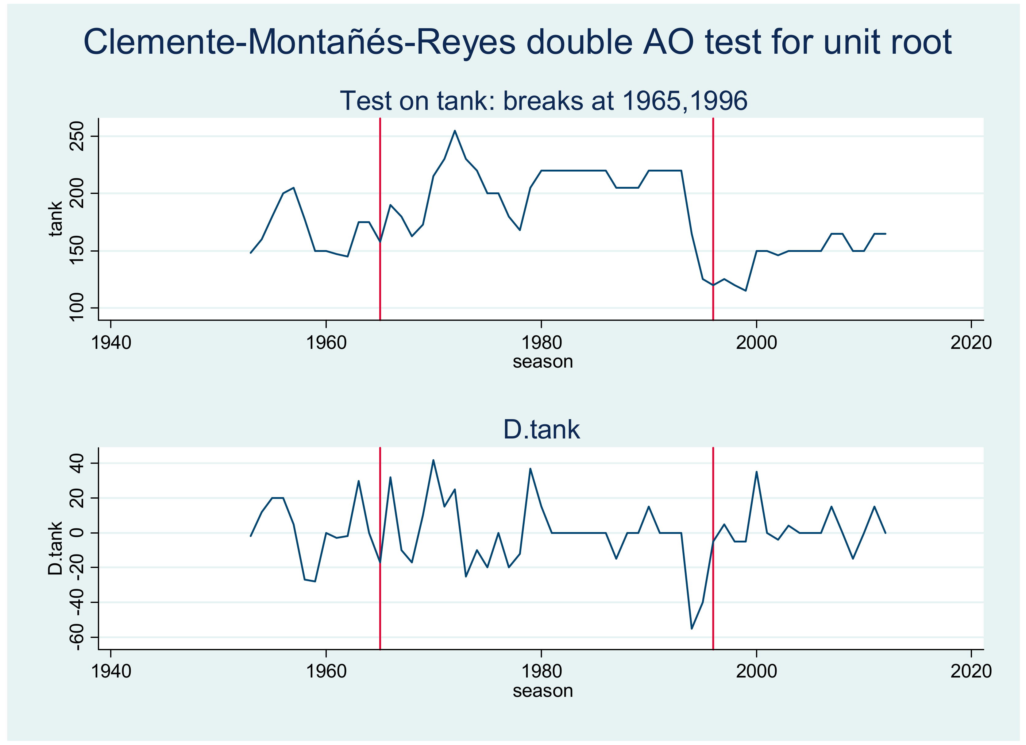
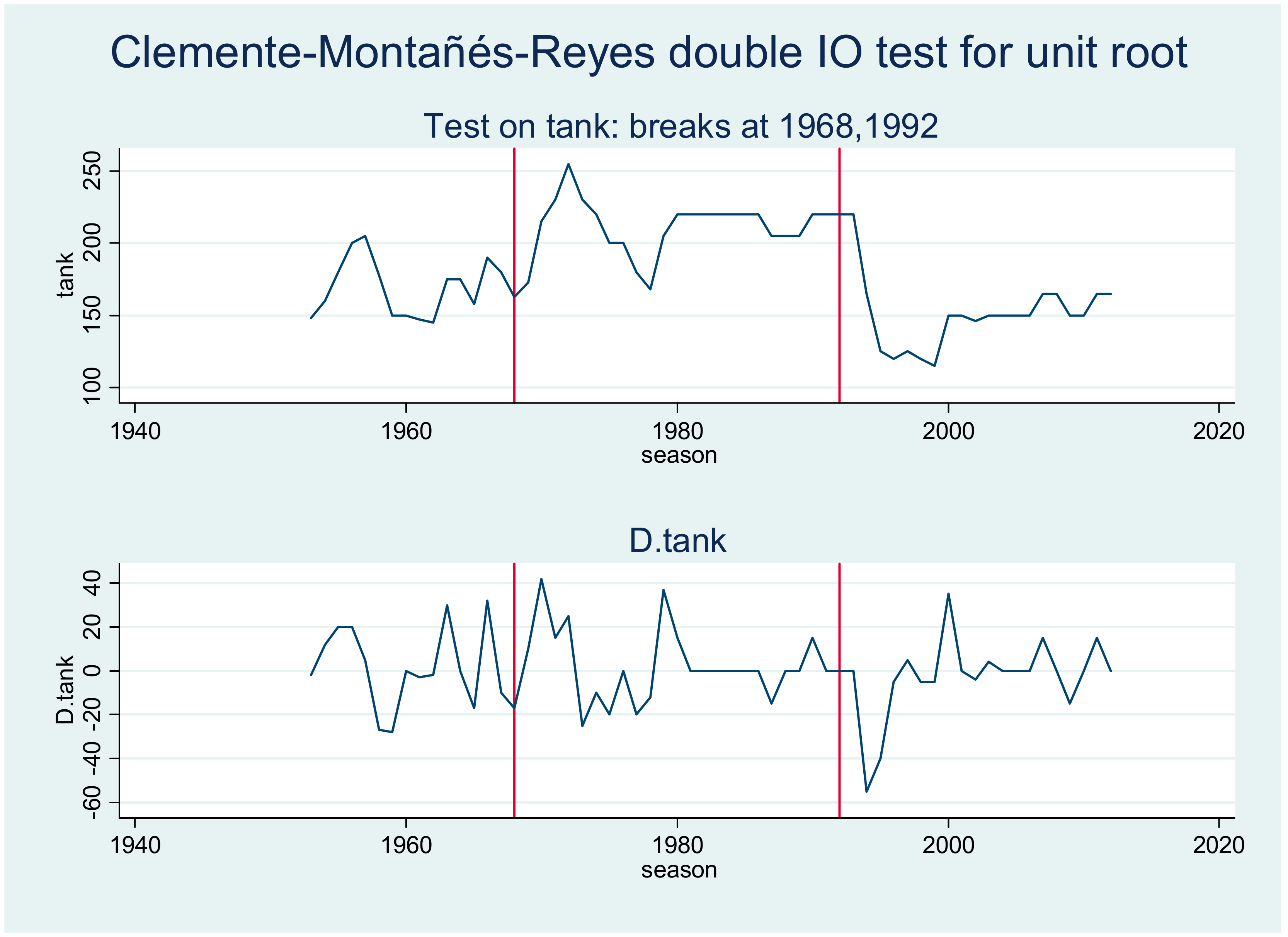
3.1. Changes in Tank Capacity

We will first observe how the tank capacity of Formula One cars has developed since 1950. As previously discussed, following several authors [32,36], the tank capacity has changed over three major dimensions: regulations about fueling/refueling across the seasons, the evolution of engines and chassis, and the evolution of admitted fuel characteristics. Our collection of data allowed us to construct Figure 2. Descriptive statistics and sources are in

Table A1. Data sources, descriptive statistics, and ADF tests.

Series	Mean	Standard Deviation	Minimum	Maximum	${\mathbf{\Delta }}^{\mathit{d}}{\mathit{y}}_{\mathit{t}}$	ADF
						No Interception; No Trend	With Interception; No Trend	With Interception; With Trend
Tank capacity, median (Source: a, b, c)	177.82	33.71	115	255	d = 0	−0.33 (1)	−2.73 *(1)	−2.86 (2)
					d = 1	−5.02 ***(2)	−4.98 ***(2)	−4.99 ***(2)
Average # cars finishing each race (Source: d)	14.64	4.00	7	23.21	d = 0	−0.264(2)	−3.24 **(1)	−3.57 **(2)
					d = 1	−8.15 ***(1)	−8.10 ***(1)	−8.02 ***(1)
Consumed fuel (liters) (1950–2015) (Source: Monte-Carlo simulations upon Sources a, b, c, and d).	2610.44	868.90	926.82	4774.87	d = 0	−0.47(1)	−2.77 *(1)	−2.78(1)
					d = 1	−7.75 ***(1)	−7.70 ***(1)	−7.65 ***(1)
CO2, log (Kg) (1950–2015) (Source: Monte-Carlo simulations upon Sources a, b, c, d, and e)	6043.44	2011.60	2145.68	11,054.32	d = 0	−0.47(1)	−2.77 *(1)	−2.78(2)
					d = 1	−7.75 ***(1)	−7.70 ***(1)	−7.65 ***(1)

Legend—Significance level: * 10%; ** 5%; *** 1%. Between parentheses, the optimal number of lags according to Schwarz criteria; Sources—a: Cimarosti [33]. b: [58] c [59] d: [60] e: [43].

(Appendix A).

Figure 2 expresses the evolution of the median F1 car’s tank capacity for each season. In the first seasons, the mean values for the F1 cars’ tank capacity raised from 150 L to 200 L (in 1957). Some of the cars with the largest tanks (more than 270 L of capacity) were the March 711 (in 1971), while other cars, like the Tyrrell 024 (in 1996), exhibited significantly lower values. The last seasons of the 1960s witnessed a persistent movement of a “race to fuel” because of the increasing revenues coming from sponsorship (Cimarosti [33]), leading to the appearance of cars like the March 711 with tanks having the capacity of more than 270 L. The values of the tanks’ capacity remained high until the first seasons of the 1990s. This was a decade characterized by an evident decrease of these values. Actually, in the 2000 season, the median tank had a capacity below 150 L.

However, just a descriptive paragraph is not sufficient. As we intend to go a step forward, we have to observe the most important moments of significant changes in the cars’ tank capacity (and correlated in the fuel consumption and CO₂ emissions per race and per season). Thus, for this section, we tested precise structural breaks for F1 car tank capacities between 1950 and 2015.

The history of the analysis of structural breaks in time series is well documented in works like Aue and Horvath [45] or Lu and Ito [46]. From the first generations, focused on testing the statistical significance of structural breaks identified for precise moments (like the Chow test), we now have tests for unknown dates. Within these modern tests, we find the tests for multiple time breaks, like Clemente et al. [47], whose critical values were previously suggested by Perron and Vogelsang [48]. The test of Clemente et al. [47] allows us to discuss the nature of the break, highlighting the difference between sudden breaks in the series (“additive outliers”) or smooth changes (“innovational outliers”). As Mourao and Martinho [49] asserted, tests like that of Clemente et al. [47] have additional convenience properties because they do not have so many restrictions on the stationarity of the series as tests like Bai and Perron [50] that imposed, for instances, that the series must be I(0) (i.e., stationary at the levels).

According to Clemente et al. [47], and to the forms used by Baum [51], b_t refers to our series of the median tank capacity of F1 cars for each season (t) between 1950 and 2015. To test the presence of multiple additive outliers, we estimated the following system of Equation (1):

$$\begin{array}{l}{b}_t=\alpha +{\delta }_{1}D{U}_{1t}+{\delta }_{2}D{U}_{2t}+e_t\\ e_t={\displaystyle \sum _{i=1}^k{w}_{1i}D{T}_{b1,t-i}+}{\displaystyle \sum _{i=1}^k{w}_{2i}D{T}_{b2,t-i}+}\rho e_{t-i}+{\displaystyle \sum _{i=1}^k{\theta }_i\Delta e_{t-i}+z_t}\end{array}$$

(1)

DU_1t = 1 for the season t after the first break time and zero. Equivalently, DU_2t is equal to 1 for the season t after the second break time and zero. T_b1 and T_b2 identify the breakpoints to be located by grid search (i.e., by identifying the minimal t-ratio for the hypothesis $\rho$ = 1). Following Baum (2005), we used DT_bm,t = 1 for t = T_bm+1 and 0 for m = 1, 2.

To test $\rho$ = 1 with the presence of innovational outliers, we teste the following model (Baum [51]):

$$\begin{array}{l}{b}_t=\alpha +{\delta }_{1}D{U}_{1t}+{\delta }_{2}D{U}_{2t}+w_{1}D{T}_{b1,t}+w_{2}D{T}_{b2,t}+\alpha b_{t-i}+{\displaystyle \sum _{i=1}^k{\theta }_i\Delta b_{t-i}+z_t}\\ \end{array}$$

(2)

Table 2. Clemente et al.’s [47] test of the F1 cars’ tank capacity.

Series	Break Assumption	Optimal Breakpoints	t-Statistic (AR-n)
Tank capacity (liters) (1950–2015)	Additive Outliers	1965 1996	4.961 *** (AR-1) −7.069 *** (AR-1)
	Innovational Outliers	1968 1992	5.751 *** (AR-3) −7.070 *** (AR-3)

Note: significance level: *** 1%.

shows the results from the tests of Clemente et al. [47] on the series of F1 car tank capacities (1950–2015). Figure 3 and Figure 4 were generated using Stata’s clemao2 and clemio2 routines.

Table 2 and Figure 2 and Figure 3 suggest that the series composed by the median values for the tank capacity of F1 cars has two breakpoints. The first occurs between the 1965 (if assuming additive outliers) and 1968 seasons (if assuming innovational outliers). The second breakpoint occurs between the 1992 (if assuming innovational outliers) and 1996 seasons (if assuming additive outliers).

The seasons of the first identified period (1965–1968) are associated with important changes in the regulations for F1 engines. Supercharging was allowed after a period in which it had been banned. (Formula One regulations banned the supercharged 3.0 L V12 engines until the 1950s. A good representative of those banned engines are the engines by Auto Union or Mercedes-Benz during the 1930s.) In practical terms, engines’ capacity increased to 3.0 L atmospheric and 1.5 L supercharged engines. The 1966 season was even recognized as a transitional year, with 2.0 L versions of the BRM and Coventry-Climax V8 engines. In the following season (1967), the popularity of the Cosworth DFV engines allowed a higher heterogeneity of manufacturers in the grid (Atlas F1, 2000).

The second identified period (1992–1996) also had important changes in the regulations of Formula One. Ferrari introduced a pioneering change, substituting the V12 engines with smaller and lighter ones (the V10). After Ferrari, other “scuderias” adopted smaller and lighter engines, which allowed the appearance of smaller tanks. This evolution proved that smaller and lighter engines were not an impossibility for the future achievement of more power. (Ferrari’s 047D engine produced over 800 horsepower in 1998; the BMW P82, in the Williams chassis of 2002, hit a peak speed of 19,050 RPM.) Cimarosti [33] recognized that “each Grand Prix car needed 220 L” until 1992. After 1995, new regulations aimed at reducing power (the stroke was reduced from 3500 cc to 3000 cc). In terms of tank capacity, Cimarosti [33] recognized in the period after 1995 that “Most of the cars could take about 140 L, and capacities ranged from Simtek’s 90 L to Benetton’s 150 L”.

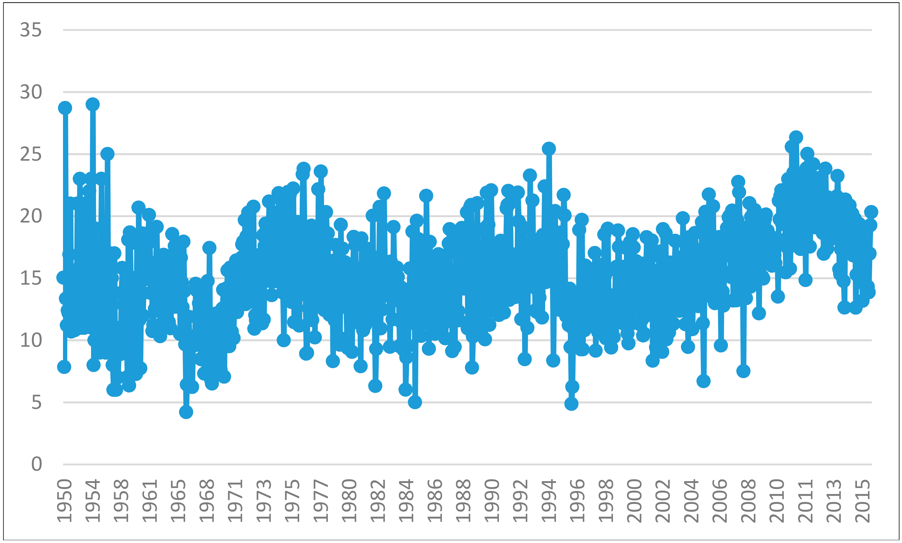
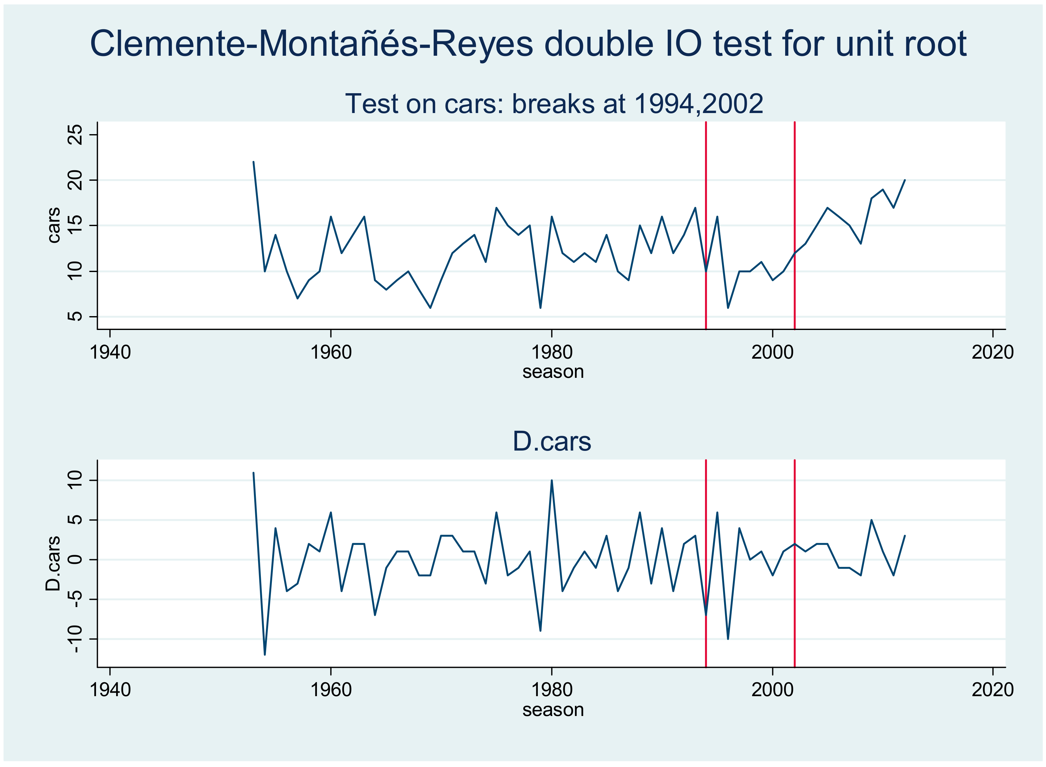
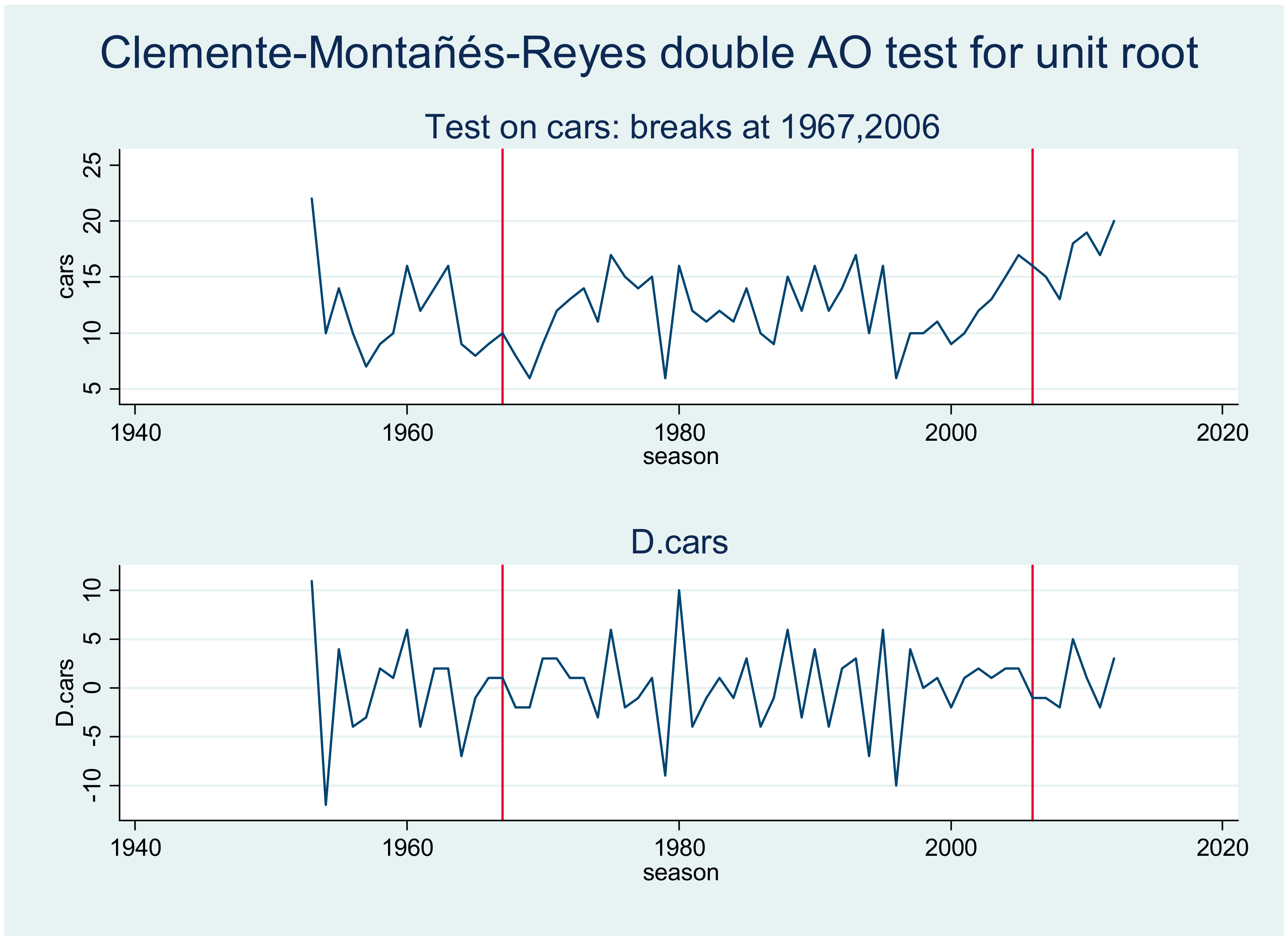
3.2. Changes in the Number of Cars Finishing Races

Following official data (Formula 1 [52]), we were able to observe the number of cars that actually finished each race. This is an important observation for supporting the estimation of the number of consumed liters of fuel and for further estimating the volume of CO₂ emitted per race. For Figure 5, we decided a car that finished the race counted as 1, a car that only raced one-half of the race counted as 0.5, and so on.

According to our method, the race with the maximum number of cars was Indianapolis/1954, with 29 cars finishing (actually, 11 cars finished the 200 laps and the remaining 22 cars summed approximately 3600 completed laps, which are equivalent to 18 cars finishing that race). Using the same approach, the minimum record was checked at Monaco/1966, with 4.21 cars finishing. There has been a certain oscillatory movement of the series, described in Figure 4, with rising numbers of cars finishing each race in the 1965–1975, 1984–1994, and 2000–2011 periods. The 1975–1984 and 1994-2000 periods can be described by downtrends in the variable related to the number of cars finishing the races. Full statistics are in Table A1.

As done in Section 3.1, we studied the presence of statistically significant breaks in the series of the average number of cars finishing each race in each season between 1950 and 2015 (Figure 6 and Figure 7 and

Table 3. Clemente et al.’s [47] test of the number of F1 cars finishing the races.

Series	Break Assumption	Optimal Breakpoints	t-Statistic (AR-n)
# cars (1950–2015)	Additive Outliers	1967 2006	0.582 (AR-1) 3.626 *** (AR-1)
	Innovational Outliers	−	−1.703 * (AR-0)4.070 *** (AR-0)

Note: significance level: * 10%; *** 1%.

).

The analysis following the results from the test of Clemente et al. [47] identified 1994 as related to the beginning of a downtrend (significant at 10% if testing innovational outliers), or the 2002–2006 period as related to the start of an uptrend.

These values converge with the explanations of Cimarosti [33], which highlight how the development of more reliable engines, chassis, and the financial status of the entrant teams in the 2000s contributed to an increased number of cars finishing the Formula One races.

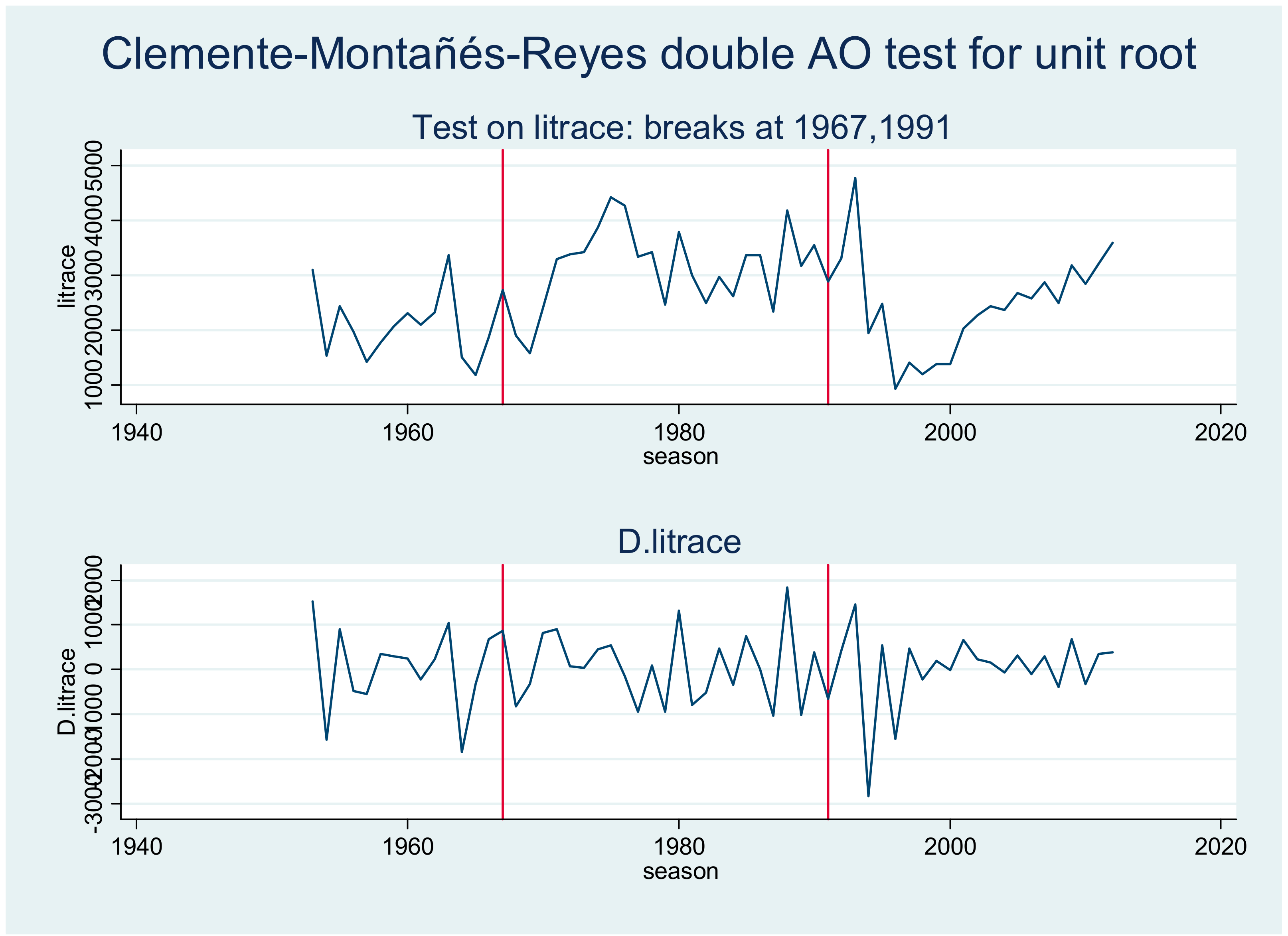
3.3. Changes in Fuel Consumption

Collecting data from Formula 1 [52], we were able to observe how many cars participated in each Formula One race and how many laps they actually ran. The literature (Madier [53]) shows there is a high probability each tank’s capacity is completely used for each race if the car finishes the race (especially in the periods in which refueling was banned); conversely, if the car only ran half of the race, it was assumed that it used half of the maximum amount of fuel carried in the tank.

For clarification, we have only considered the fuel usage by F1 cars during Sunday races (which tend to represent between one-third and one-half of the entire usage by F1 cars during the entire weekend). Total Sportek2 [54] should be referenced to achieve an estimate of the fuel usage for a season. This would get values between 200,000 and 250,000 L of fuel per team.

We then ran a Monte Carlo simulation composed of 10,000 iterations that considered the observed variables (maximum/minimum/mean/standard deviation of the capacity of the tank and maximum/minimum/mean/standard deviation of the percentage of the Sunday races run by the engine. (Values available upon request. Monte Carlo simulation allows to analyze by building models of possible results by substituting a range of values—a probability distribution—for a factor that has inherent uncertainty (in our model, number of cars finishing each race, the tanks’ capacity, and finally the CO₂ emission). It then computes results over and over, each time using a different combination of random values from the probability functions. Depending upon the number of uncertainties and the ranges specified for them, a Monte Carlo simulation could involve thousands or tens of thousands of recalculations before it is complete. However, a higher number of Monte Carlo simulations must be read as a more reliable outcome, which will generate a more probable range of expectable values.)) Analyzing the 10,000 iterations, we got a central value for the total number of liters of fuel consumed by the starting cars for each of the 916 Sunday races between Silverstone/1950 and Abu Dhabi/2015. Figure 8 exhibits the estimated range of values (confidence level of 95%) for this computation for each race of each Formula One season.

Figure 8 shows that the consumption of fuel during Sunday races increases during the 1970s and starts to decrease in 1990. Recall that, before the 1970s, there were few cars finishing the race (the mean value was 11 cars finishing the races before 1970 compared to a mean value of 14 after 1970). (The differences between these means is statistically significant (p-value lower than 0.01). Full details available upon request.) This explains the low values (around 2000 L consumed by all cars per race) found for the period before 1970. However, the reliability of chassis and engines has significantly evolved since then (Wright [36]), which could explain the rising trend and the stable values after 1970 (in some races in this period, there were estimated peaks above 5000 L). However, the simultaneous race to efficiency by F1 teams, combined with the restrictive regulations, proportionated lower consumptions of fuel per race, especially after the 1990s. (For 2008, the average rate of consumption for F1 cars ranged between 68.0 and 72.9 L per 100 km. Our values also converge to estimates on the value of fuel consumed per F1 race, like those of Venkatesan [55].)

As done with the series composed by the average values for F1 tan capacities, we also studied the existence of breaks for the series composed by the average value of consumed liters of fuel for each F1 season races.

Table 4. Clemente et al.’s [47] test of liters of fuel consumed by race.

Series	Break Assumption	Optimal Breakpoints	t-Statistic (AR-n)
Consumed fuel (liters) (1950–2015)	Additive Outliers	1967 1991	4.651 *** (AR-4) −2.921 *** (AR-4)
	Innovational Outliers	1968 1992	3.793 *** (AR-5) −3.432 *** (AR-5)

Note: significance level: *** 1%.

and Figure 8 and Figure 9 show the results from the tests of Clemente et al. [47] on the series of the estimated number of consumed liters of fuel for each F1 race (1950–2015). Figure 9 and Figure 10 were generated using Stata’s clemao2 and clemio2 routines.

The values suggested by Table 4 and Figure 8 and Figure 9 identify two periods associated to statistically significant breaks in the values for the number of liters consumed per F1 race. The first period is identified in the 1967 (assuming additive outliers) or 1968 seasons (assuming innovational outliers). The second period is identified in the 1991 (assuming additive outliers) or 1992 seasons (assuming innovational outliers).

Cimarosti [33] wrote that most research and development in Formula One up to 1966 particularly enhanced the manufacture of chassis and engines, but also raised concerns with safety, moving towards reduced vehicle weight with use of titanium and magnesium alloys. The same author (Cimarosti [33]) also showed this as the period (1966–1970) of Formula One cars of the 3-litre formula. These cars had values significantly higher in capacity, bore, binary horsepower, and weight if compared to the cars of the previous periods. These higher values resulted in higher consumption of fuel oil, which follows Arron [56] or Hynes [57].

However, for the second period of structural breaks (1991–1992), Cimarosti [33] suggested that the political instability resulting from the Gulf War fostered the adoption of limits on fuel: a maximum of 102 ROZ, 2% oxygen at the most, a maximum of 0.2% hydrogen, and no more than 5% benzoyl (numbers that were revised in 1992 in a more restricted way). Cars usually started the races with 210–220 L of fuel.

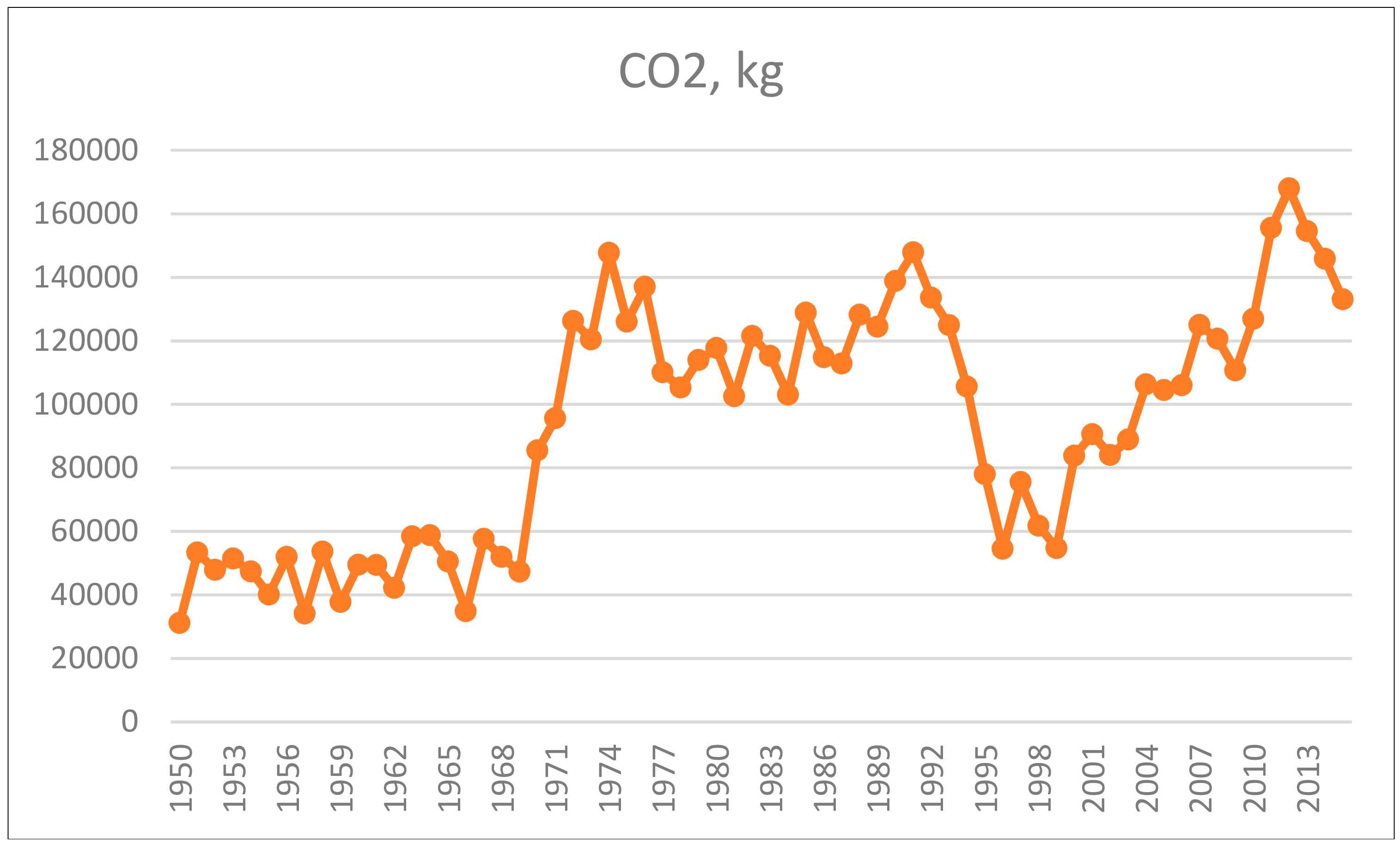
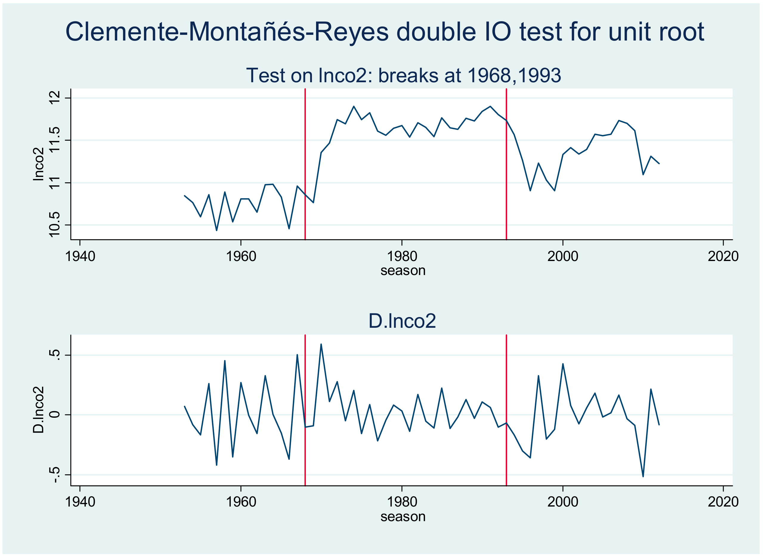
3.4. Changes in CO₂ Emissions

After determining an estimate for the liters of fuel consumed per Sunday race, we were able to estimate the quantity of CO₂ emitted by F1 cars per race. (Recall that, according to the Trucost Report [31], “Only a small proportion, 0.3% [of CO₂ due to Formula One], arises from the fuel consumed in the race itself and testing of the cars at the race.” The same source “indicates that the majority of greenhouse gas emissions arise from the production and supply of raw materials and parts for the teams.”) Recall that 1 L of petrol corresponds to an estimated value of 2.3151 km of CO₂ (EIA [43]). However, the presence of additives or substances like kerosene increases this correspondence by a rate of approximately 12.64%. Once again, we ran 10,000 Monte Carlo iterations, which resulted in Figure 11.

Summing the central value estimated for each race, we determined an estimated value for the CO₂ emitted by Sunday races for each season in F1 (Figure 12).

In Figure 12, we observe significantly higher values during the seasons between 1970 and 1992 (the period dominated by the turbochargers and Cosworth engines). After six seasons of downtrend after 1992, Figure 11 suggests the existence of an uptrend for the estimated value of kilograms of emitted CO₂ starting in the last seasons of the 1990s, which has reverted since 2012.

Compared to Figure 1 (CO₂ emissions by sector), Figure 12 suggests a different pattern. Actually, Figure 11 exhibits a period of higher control/even reduction of CO₂ emissions in a specific motorsport (Formula One); conversely, Figure 1 suggests a persistent uptrend in CO₂ emissions, especially for the entire transportation sector. This distinction is additional proof of the particular efforts of this expensive motorsport in carbon reduction.

As previously done, we also estimated the structural breaks for the estimated CO₂ emissions in Sunday races for each season in F1.

Table 5. Clemente et al.’s [47] test of kilograms of CO₂ emitted by season (Sunday’s races).

Series	Break Assumption	Optimal Breakpoints	t-Statistic (AR-n)
CO2, log (Kg) (1950–2015)	Additive Outliers	1967 1994	11.878 *** (AR-12) −4.242 *** (AR-12)
	Innovational Outliers	1968 1993	6.064 *** (AR-9) −4.568 *** (AR-9)

Note: significance level: *** 1%.

and Figure 12 and Figure 13 show the results from the tests of Clemente et al. [47] on the series of the estimated quantity of emitted CO₂ in Sunday races for each F1 season (1950–2015). Figure 12 and Figure 13 were generated using Stata’s clemao2 and clemio2 routines of Stata 12.0.

Once again, the 1967/1968 and 1993/1994 periods are identified as structural breaks, but now regarding the series of the estimated values for the emitted CO₂ per season and only considering the Sunday Formula One races. Besides the already discussed dimensions behind the identification of these breaks in the previously commented series, we must consider the increasing number of races in each season since 1970 and the notorious reliability of the cars and engines. On the one hand, this increased the length of the seasons (and obviously the number of races); on the other hand, this led to a higher number of cars completing more laps (as mentioned for Figure 14).

However, we have two additional comments for Table 5 and Figure 12 and Figure 13. The first regards the values achieved for the optimal number of lags used for getting the values of Table 5: 12 (additive outliers) or 9 (innovational outliers). These values are the highest among the values chosen for all tests on structural breaks presented in this paper. This evidence suggests the particular persistence of the estimated values for the CO₂ emitted per F1 race, being an alternative evidence of the delayed effects of CO₂ emissions, even if recorded at motorsports. The second comment shows the (still) low relevance of the deep changes introduced in F1 regulations regarding the control of the F1 carbon footprint, especially since 2010–2011. Actually, our tests did not return significant values for this period, allowing us to characterize it as a structural break. However, we do not deny the possibility of revising this comment after collecting more data, as new seasons are being organized and incorporated in our data sample.

4. Conclusions and Research Challenges

Motorsports and, in particular, Formula One, only run with a substantial amount of resources, including carbon footprint. Investors, shareholders, sponsors, and fans of today’s sports expect motorsports teams to be simultaneously competitive and proactive in the search for more sustainable races in terms of CO₂ emissions, fuel usage, engine longevity, treatment of residuals, and technological advancement. Although Formula One (and its ecologically engagée relative, the Formula E) is far from the concept of “fuel neutral races” (where teams can only use the fuel that they have generated), there have been notorious advances since 1950 (the first season organized by FIA) in terms of engine efficiency, control of pollutant gases, and fuel recipes.

This paper is the first to empirically estimate the levels of CO₂ emitted by F1 cars during Sunday races. This estimation was done for all seasons before 2016. As a first step, there was data collection from official sources. We collected data for the F1 cars’ tank capacity and for the number of cars finishing the races. Then, using Monte Carlo iterations, we estimated the number of consumed liters of fuel per race and the level of CO₂ corresponding to this value of consumed liters.

For each of these series, we additionally studied the stationarity profile and the related structural breaks. In a general observation, the period of the dominance of the turbochargers and Cosworth engines was identified as a period of higher CO₂ emissions. The 5-year period after 1992, characterized by lighter engines, also became associated as a period of decreased emissions. Although deep changes towards a more ecologically sustainable sport were introduced in Formula One’s regulations in the recent 2009–2011 period, our analysis did not detect a significant change in the global level of CO₂ emitted by F1 cars during Sunday races.

Some research challenges emerge from this paper. One relates to an enlargement of the focus of this paper, which only considers the CO₂ emissions of F1 cars during Sunday races. Therefore, we consider observing the emissions from F1 cars during entire race weekends as a relevant extension. Another challenge comes from applying the methodology used here to other motorsports in order to have a clarified perspective of the carbon footprint of these widely appreciated sports. Finally, a third challenge regards the opportunity of detailing the rhythm of changes in motorsports when compared to the changes in the transportation or road sectors in terms of control of the pollutant gases.

References

1. Fulton, L.; Mejia, A.; Arioli, M.; Dematera, K.; Lah, O. Climate Change Mitigation Pathways for Southeast Asia: CO2 Emissions Reduction Policies for the Energy and Transport Sectors. Sustainability 2017, 9, 1160. [Google Scholar] [CrossRef]
2. Centobelli, P.; Cerchione, R.; Esposito, E. Developing the WH2 framework for environmental sustainability in logistics service providers: A taxonomy of green initiatives. J. Clean. Prod. 2017, 165, 1063–1077. [Google Scholar] [CrossRef]
3. Tso, G.; Guan, J. A multilevel regression approach to understand effects of environment indicators and household features on residential energy consumption. Energy 2014, 66, 722–731. [Google Scholar] [CrossRef]
4. Marquart-Pyatt, S. Contextual Influences on Environmental Concern Cross-Nationally: A Multilevel Investigation. Soc. Sci. Res. 2012, 41, 1085–1099. [Google Scholar] [CrossRef] [PubMed]
5. Eurobarometer. First Results May 2008. Available online: http://ec.europa.eu/public_opinion/archives/eb/eb69/eb_69_first_en.pdf (accessed on 23 November 2017).
6. Carvalho, M.; Bonifacio, M.; Dechamps, P. Building a low carbon society. Energy 2011, 36, 1842–1847. [Google Scholar] [CrossRef]
7. Yearley, S. Bridging the science-policy divide in urban air-quality management: Evaluating ways to make models more robust through public engagement. Environ. Plan. C 2006, 24, 701. [Google Scholar] [CrossRef]
8. Brechin, S.; Kempton, W. Beyond Postmaterialist Values: National versus Individual Explanations of Global Environmentalism. Soc. Sci. Q. 1997, 78, 16–20. [Google Scholar]
9. Prescott-Clarke, P.; Mostyn, B. Public Attitudes towards Industrial, Work Related and Other Risks; Social and Community Planning Research: London, UK, 1982. [Google Scholar]
10. Ahmad, N.; Du, L.; Lu, J.; Wang, J.; Li, H.; Hashmi, M. Modelling the CO2 emissions and economic growth in Croatia: Is there any environmental Kuznets curve? Energy 2017, 123, 164–172. [Google Scholar] [CrossRef]
11. Steen, M. Greenhouse Gas Emissions from Fossil Fuel Fired Power Generation Systems; Joint Research Centre/European Comission: Brussels, Belgium, 2001. [Google Scholar]
12. Olabi, A. 100% sustainable energy. Energy 2014, 77, 1–5. [Google Scholar] [CrossRef]
13. Gillingham, K.; Newell, R.; Palmer, K. Energy Efficiency Economics and Policy. Annu. Rev. Resour. Econ. 2009, 1, 597–620. [Google Scholar] [CrossRef] [Green Version]
14. Gallego, F.; Montero, J.; Salas, C. The effect of transport policies on car use: A bundling model with applications. Energy Econ. 2013, 40, 85S–97S. [Google Scholar] [CrossRef]
15. EPA Sources of Greenhouse Gas Emissions. Available online: https://www.epa.gov/ghgemissions/sources-greenhouse-gas-emissions (accessed on 23 November 2017).
16. OECD/IEA. CO2 Emissions from Fuel Combustion; OECD/International Energy Agency: Paris, France, 2016. [Google Scholar]
17. Voltes-Dorta, A.; Perdiguero, J.; Jimenez, J. Are car manufacturers on the way to reduce CO2 emissions?: A DEA approach. Energy Econ. 2013, 38, 77–86. [Google Scholar] [CrossRef] [Green Version]
18. Storchmann, K. Long-Run Gasoline demand for passenger cars: The role of income distribution. Energy Econ. 2005, 27, 25–58. [Google Scholar] [CrossRef]
19. Falco, C.; Donzelli, F.; Olper, A. Climate Change, Agriculture and Migration: A Survey. Sustainability 2018, 10, 1405. [Google Scholar] [CrossRef]
20. Nichols, A.; Maynard, V.; Goodman, B.; Richardson, J. Health, Climate Change and Sustainability: A systematic Review and Thematic Analysis of the Literature. Environ. Health Insights 2009, 3, 63–88. [Google Scholar] [CrossRef] [PubMed]
21. Broto, V.; Bulkeley, H. A survey of urban climate change experiments in 100 cities. Glob. Environ. Chang. 2013, 23, 92–102. [Google Scholar] [CrossRef] [PubMed] [Green Version]
22. Alnaser, W.; Probert, S.; El-Masri, S.; Al-Khalifa, S.; Flanagan, R.; Alnaser, N. Bahrain’s Formula-1 racing circuit: Energy and environmental considerations. Appl. Energy 2006, 83, 352–370. [Google Scholar] [CrossRef]
23. Kravchenko, M.; Nosov, I. Motorsport and Sustainability: Case Study of MXStar Team’s Environmental Impact Optimization. Master’s Thesis, Uppsala Universitet, Uppsala, Sweden, 2011. [Google Scholar]
24. Clerides, S.; Zachariadis, T. The effect of standards and fuel prices on automobile fuel economy: An international analysis. Energy Econ. 2008, 30, 2657–2672. [Google Scholar] [CrossRef]
25. Allen, J. F1 Sponsors and Supporters Drive the Shift to Sustainability. Financial Times, 13 March 2014. [Google Scholar]
26. Global Sports Impact Report 2016; Sportcal, Market Intelligence: London, UK, 2016.
27. Coalter, F.; Taylor, J. Large Scale Sports Events: Event Impact Framework; Report to UK Sport; Department of Sports Studies, University of Stirling: Stirling, UK, 2008. [Google Scholar]
28. Ornstein, D. Earth Car or not, Button will emit over 50 tonnes of CO2 this season. The Guardian, 2 March 2007. [Google Scholar]
29. Ornstein, D. Formula 1 testing in Barcelona, day two as it happened. BBC Sport, 9 March 2011. [Google Scholar]
30. Purcell, A. McLaren F1 team goes carbon neutral. New Scientist, 8 December 2011. [Google Scholar]
31. TRUCOST. FOTA Environment Programme Baseline Report. Formula One Teams Association, Geneva. 2011. Available online: http://www.f1fanatic.co.uk/wp-content/uploads/2010/06/FOTA-Environment-Programme-Baseline-Report-2010.pdf (accessed on 23 November 2017).
32. Galvin, R. How does speed affect the rebound effect in car travel? Conceptual issues explored in case study of 900 Formula 1 Grand Prix speed trials. Energy 2017, 128, 28–38. [Google Scholar] [CrossRef]
33. Cimarosti, A. The Complete History of Grand Prix Motor Racing; Aurum Press: London, UK, 1997. [Google Scholar]
34. Mack, J.; Schuler, D.; Butt, R.; Dibble, R. Experimental investigation of butanol isomer combustion in Homogeneous Charge Compression Ignition (HCCI) engines. Appl. Energy 2016, 165, 612–626. [Google Scholar] [CrossRef]
35. Grez, M. Formula One Fuel’s Hidden 1%: The Best Kept Secret in Sport? Available online: http://edition.cnn.com/2015/07/24/motorsport/formula-one-fuel/ (accessed on 23 November 2017).
36. Wright, P. Formula 1 Technology; Society of Automotive Engineers: Troy, MI, USA, 2001. [Google Scholar]
37. Fagnan, R. F1 Technical: Fuel Tanks Explained. Available online: https://www.auto123.com/en/racing-news/f1-technical-fuel-tanks-explained?artid=109115&pg=2 (accessed on 23 November 2017).
38. Edmondson, L. Is an F1 Car More Energy Efficient than an Electric Vehicle? Available online: http://www.espn.co.uk/f1/story/_/id/15152695/is-f1-car-more-energy-efficient-electric-vehicle (accessed on 23 November 2017).
39. Taylor, L. Straw from Area Farmers Helps Fuel Ferrari’s F1 Dream Machines. Available online: http://www.iogen.ca/media-resources/iogen_news/2010_03_15_citizen.pdf (accessed on 23 November 2017).
40. De Groote, S. Fuel. F1 Technical. Available online: http://www.f1technical.net/articles/19 (accessed on 23 November 2017).
41. Flagan, R.C.; Seinfeld, J.H. Fundamentals of Air Pollution Engineering; Prentice-Hall Inc.: Upper Saddle River, NJ, USA, 1988; p. 542. [Google Scholar]
42. Larsen, U.; Johansen, T.; Schramm, J. Ethanol as a Fuel for Road Transportation; IEA-AMF Report; 2009. [Google Scholar]
43. Energy Information Administration. Carbon Dioxide Emissions Coefficients. 2016. Available online: https://www.eia.gov/environment/emissions/co2_vol_mass.cfm (accessed on 23 November 2017).
44. Atlas F1. The 80s. 2000. Available online: http://atlasf1.autosport.com/evolution/1980s.html (accessed on 23 November 2017).
45. Aue, J.; Horvath, L. Structural Breaks in Time Series. J. Time Ser. Anal. 2013, 34, 1–16. [Google Scholar] [CrossRef]
46. Lu, S.; Ito, T. Structural Breaks and Time-varying Parameter: A Survey with Application. Commun. IBIMA 2008, 2008, 100037. [Google Scholar]
47. Clemente, J.; Montañés, A.; Reyes, M. Testing for a unit root in variables with a double change in the mean. Econ. Lett. 1998, 59, 175–182. [Google Scholar] [CrossRef]
48. Perron, P.; Vogelsang, T. Nonstationarity and level shifts with an application to purchasing power parity. J. Bus. Econ. Stat. 1992, 10, 301–320. [Google Scholar]
49. Mourao, P.; Martinho, V. Discussing structural breaks in the Portuguese regulation on forestfires—An economic approach. Land Use Policy 2016, 54, 460–478. [Google Scholar] [CrossRef]
50. Bai, J.; Perron, P. Critical values for multiple structural change tests. Econ. J. 2003, 6, 72–78. [Google Scholar] [CrossRef]
51. Baum, C. Stata: The language of choice for time-series analysis? Stata J. 2015, 5, 46–63. [Google Scholar]
52. Formula 1. Various Databases. Available online: http://www.formula1.com (accessed on 23 November 2017).
53. Madier, D. The Formula 1 Hybrid Power Units 2014–2015. F1 Forecast. Available online: http://www.f1-forecast.com/pdf/The%20Formula%201%20Hybrid%20Power%20Units%202014-2015.pdf (accessed on 23 November 2017).
54. Total Sportek2. How Much a Formula One Car Cost (Component Wise Price). Total Sportek2. 17 December 2014. Available online: http://www.totalsportek.com/f1/how-much-formula-1-car-cost-in-2015/ (accessed on 23 November 2017).
55. Venkatesan How Much Fuel Is Consumed in One F1 Race. Available online: https://www.quora.com/How-much-fuel-is-consumed-in-one-F1-race (accessed on 23 November 2017).
56. Arron, S. Crucial Brews. The Telegraph. 6 July 2002. Available online: http://www.telegraph.co.uk/motoring/4757155/Crucial-brews.html (accessed on 23 November 2017).
57. Hynes, D. Formula One’s Eldest Statesman. AUTO Int. J. FIA 2014, 7, 66–68. [Google Scholar]
58. Webcarstory. Various pages. Available online: http://www.webcarstory.com/?width=1152 (accessed on 23 November 2017).
59. Wikipedia. Various pages. Available online: http://www.wikipedia.org (accessed on 23 November 2017).
60. Formula 1. Various pages. Available online: https://www.formula1.com/ (accessed on 23 November 2017).
Figure 1. CO2 emissions by sector. Source: OECD/IEA [16].
Sustainability 10 01841 g001
Figure 2. Median F1 car’s tank capacity (liters, at the vertical axis) along F1 seasons.
Sustainability 10 01841 g002
Figure 3. Additive outliers test for unit root (series: median F1 tank capacity). Legend: at the vertical axes, the units are number of liters (first panel) and difference from the previous season in number of liters (second panel); at the horizontal axes, the units refer to the year of each season.
Sustainability 10 01841 g003
Figure 4. Innovational outliers test for unit root (series: median F1 tank capacity). Legend: at the vertical axes, the units are number of liters (first panel) and difference from the previous season in number of liters (second panel); at the horizontal axes, the units refer to the year of each season.
Sustainability 10 01841 g004
Figure 5. Number of cars finishing each F1 race. Legend: at the vertical axis, the units are number of cars finishing each F1 race/season; at the horizontal axis, the units are the years of the seasons.
Sustainability 10 01841 g005
Figure 6. Innovational outliers test for unit root (series: avg. number of cars finishing each race in the season). Legend: at the vertical axes, the units are number of cars finishing each season’s race on average (first panel) and difference from the previous season in number of cars finishing each season’s race (second panel); at the horizontal axes, the units refer to the year of each season.
Sustainability 10 01841 g006
Figure 7. Additive outliers test for unit root (series: avg. number of cars finishing each race in the season). Legend: at the vertical axes, the units are number of cars finishing each season’s race on average (first panel) and difference from the previous season in number of cars finishing each season’s race (second panel); at the horizontal axes, the units refer to the year of each season.
Sustainability 10 01841 g007
Figure 8. Total liters of fuel consumed per F1 Sunday’s race. Legend: at the vertical axes, the units are range of values for the estimated value of fuel consumed per F1 race; at the horizontal axes, the units refer to the year of each season.
Sustainability 10 01841 g008
Figure 9. Innovational outliers test for unit root (series: consumed fuel per F1 cars during Sunday’s races). Legend: at the vertical axes, the units are consumed fuel per F1 Sunday’s races (first panel) and difference from the previous season in consumed fuel per F1 Sunday’s race (second panel); at the horizontal axes, the units refer to the year of each season.
Sustainability 10 01841 g009
Figure 10. Additive outliers test for unit root (series: consumed fuel per F1 cars during Sunday’s races). Legend: at the vertical axes, the units are consumed fuel per F1 Sunday’s races (first panel) and difference to previous season in consumed fuel per F1 Sunday’s race (second panel); at the horizontal axes, the units refer to the year of each season.
Sustainability 10 01841 g010
Figure 11. CO2 emitted, cars/Sundays’ race (kilograms, 10,000 Monte Carlo (MC) iterations). Legend: at the vertical axis, the units are estimated number of kilograms of CO2 emitted by F1 cars at Sunday’s races after 10,000 MC iterations; at the horizontal axis, the units refer to the year of each season.
Sustainability 10 01841 g011
Figure 12. CO2 emitted by F1 cars in Sundays’ race (kilograms). Legend: at the vertical axis, the units are estimated mean for the number of kilograms of CO2 emitted by F1 cars at Sunday’s races after 10,000 MC iterations; at the horizontal axis, the units refer to the year of each season.
Sustainability 10 01841 g012
Figure 13. Innovational outliers test for unit root (series: log of CO2 emitted during Sunday’s F1 races). Legend: at the vertical axes, the units are the log value of consumed fuel per F1 Sunday’s races (first panel) and difference from the previous season in the log value of consumed fuel per F1 Sunday’s race (second panel); at the horizontal axes, the units refer to the year of each season.
Sustainability 10 01841 g013
Figure 14. Additive outliers test for unit root (series: log of CO2 emitted during Sunday’s F1 races). Legend: at the vertical axes, the units are the log value of consumed fuel per F1 Sunday’s races (first panel) and difference from the previous season in the log value of consumed fuel per F1 Sunday’s race (second panel); at the horizontal axes, the units refer to the year of each season.
Sustainability 10 01841 g014