Structural Impact Relationships Between Urban Development Intensity Characteristics and Carbon Dioxide Emissions in Korea

Abstract

The goal of this study is to analyze the interrelated direct and indirect impacts of urban development intensity (UDI) characteristics on carbon dioxide (CO₂) emissions in Korea. The study also compares the main arguments and analysis results of previous studies on cities that are effective in reducing CO₂ emissions. To do this, factors attributable to the UDI characteristics of Korea were selected, and CO₂ emissions were calculated. Then, the impact of UDI characteristics on CO₂ emissions was analyzed using the partial least squares structural equation model. The main results show that the physical, spatial, and socio-demographic characteristics of UDI have a direct impact on CO₂ emissions, and physical, economic, and city-type characteristics indirectly affect CO₂ emissions. As a result, we reach the following conclusions: (i) dense urban forms reduce CO₂ emissions; (ii) economic characteristics of UDI have impact on total CO₂ emissions, having both negative and positive effects; and (iii) medium and small cities have higher per capita CO₂ emissions than do large cities.

1. Introduction

1.1. Theoretical Background

Global warming causes climate change and affects natural ecosystems, human health, residential environments, industrial activities, and socioeconomic spheres. Carbon dioxide (CO₂) has been identified by numerous scientists to be the primary cause of global warming; CO₂ emissions are especially rampant in cities, due to human activities and the burning of fossil fuels [1]. Korea ranked 7th in global CO₂ emissions in 2010, emitting 5.90 million tons; Korea also has the third largest rate of CO₂ emissions increase, with a 136% increase since 1990 [2].

In order to minimize CO₂ emissions, policymakers are turning their attention toward the development of energy conservation and emissions mitigation strategies [3]. Interest in the effects of urban development intensity (UDI) on CO₂ emissions reduction, in relation to urban planning and spatial optimization measures [4], is increasing, as urbanization is known to affect the intensity of carbon emissions activity within cities [5,6]. UDI is defined in terms of the various impacts that human development activities exert on urban areas [7].

The following studies illustrate that UDI research is being conducted in various ways, depending on the academic background and approach of the researchers, and factors with similar attributes can be categorized as physical, social, or economic characteristics, amongst others. For example, Ou et al. [4] studied the effects of land use spatial patterns and density, transportation, and communication infrastructure on CO₂ emissions. Land use patterns and density elements represent spatial characteristics, and transportation and communication infrastructure facilities exhibit physical characteristics. Similarly, Guerin et al. [8] found that factors such as age, gender, and education level, which indicate social and economic characteristics, such as income and house ownership, affect energy consumption. Brownstone and Golob [9] found that spatial characteristics, such as residential density, affect vehicle mileage and fuel consumption. Tate et al. [10] and Mendes [11] developed the UDI index based on physical characteristics, such as land coverage and infrastructure, and socio-demographic characteristics, such as census block group.

However, as pointed out by Wang et al [7], virtually no studies comprehensively address the UDI characteristics relevant to urban planning. For example, Newman and Kenworthy [6] argued that physical factors, such as transportation-related automobiles and transportation facilities, accelerate CO₂, but their research fails to include economic factors, such as price or income changes. Similarly, Talbi [12] studied the relationship between CO₂ and economic aspects, such as GDP, fuel consumption, fuel ratio, and energy efficiency, and found that the latter two are important for CO₂ emissions. However, this author did not consider the fact that energy consumption patterns or CO₂ emissions may vary due to other factors, such as age or city type. Schipper et al. [13] and Guerin, Yust and Coopet [8] considered socio-demographic and economic characteristics but limited their study of energy consumption to the residential sector. Similarly, Fragkias et al. [14] examined the relationship between city size and CO₂ emissions based on population, but they did not sufficiently address other characteristics influencing this relationship.

Though previous studies do not comprehensively address UDI characteristics, a number of studies have revealed that UDI characteristics can influence other characteristics ultimately affecting CO₂ emissions indirectly. Liu and Shen [15] stated that, although urban forms do not directly affect vehicle miles traveled or vehicle energy consumption, they can indirectly affect energy consumption through other channels. O’neill and Chen [16] determined that per capita residential energy consumption increases and transportation energy decreases with homeowner age. However, per capita energy consumption (expressed as the sum of residential and transportation energy) increases with age until reaching a maximum at age 55, after which it decreases. According to Fong et al. [17], the increasing amount of time spent at home as citizens age leads to increased residential energy consumption and decreased transportation energy.

The ability to quantify and structure UDI characteristics affecting CO₂ emissions in terms of urban planning is potentially valuable, as such research can present a logical foundation for the evaluation, distribution, and management of limited resources during the implementation of high-level, long-term policy plans (such as urban master or comprehensive planning). However, as discussed in previous studies, only a single characteristic, not knowing the structural relationship with other characteristics, and different levels of measurement among the factors that characterize it should be considered to establish integrated urban planning for CO₂ reduction. Studies on the impacts of urban form and CO₂ show good examples of these concerns. Urban form is defined as built-up areas, including the shape, size, density, and configuration of settlements. It therefore refers to the spatial arrangement of individual elements, and the interaction between the elements means a series of relationships, or flows, that integrate patterns and behaviors of the individual elements in the city. In terms of UDI, urban form is mainly measured using physical and spatial characteristics. There are discrepancies in previous research of this type as to the specific urban forms that are advantageous in terms of CO₂ emissions and energy consumption. For example, Anderson et al. [18], Banister et al. [19], and Dhakal [20] found that more compact urban forms with lower dispersion rates reduce CO₂ emissions. Conversely, Newman and Kenworthy [6], Jenks and Burgess [21], and Chiu [22] claimed that there is inadequate evidence that dense cities contribute to energy conservation. Glaeser and Kahn [23] stated that large cities with high populations have an efficiency advantage over small cities in terms of energy efficiency and CO₂ emissions. In contrast, Fragkias et al. [14], who compared CO₂ emissions from large and small cities, concluded that large cities do not have more efficient emissions.

The preceding studies highlight the variety of academic perspectives and methods employed during research on the relationship between the UDI and CO₂ emissions. However, there are almost no studies on what UDI characteristics are and how they affect CO₂ emissions from an urban planning perspective. Earlier studies are restricted to the transportation and residential sectors, as opposed to urban planning, and emphasize CO₂ emissions from direct consumption over those from indirect consumption. In addition, attempts to investigate how UDI characteristics can indirectly affect CO₂ emissions by affecting other characteristics have been insufficient. As a result, the literature is not consistent in identifying the most efficient urban form in terms of CO₂ emissions. Based on these implications, we ask the following research questions: (i) What are the UDI characteristics and factors that affect CO₂ emissions in Korea; (ii) what are the structural impact relationships between UDI characteristics and CO₂ emissions; and (iii) what is the most efficient urban form to mitigate CO₂ emissions?

Thus, it is necessary to investigate the integrated interactions between UDI characteristics and CO₂ emissions from an urban planning perspective, identify the most important relationships, and present a possible direction for policy strategy. Accordingly, the goal of this study is to analyze the interrelated direct and indirect impacts of UDI characteristics on CO₂ emissions in Korea. We also compare the main arguments and analytical results of previous studies on cities that are effective in reducing CO₂ emissions.

1.2. Research Hypotheses

By reviewing the literature, we found that existing studies related to UDI did not consider other characteristics together or missed their relationships. Before we consider these, UDI characteristics need to be classified and defined. By doing so, we can classify related factors according to their characteristics and measure them at the same level. In this regard, the urban spatial structure can explain UDI characteristics, because urban spatial structure is determined by the components of the city and their interactions [24].

Parr [25] defined urban spatial structure as multifaceted, consisting of the distribution of population, employment, built-up volumes, transportation networks, and land uses. To complement the understanding of urban spatial structure, this morphological dimension can be completed by functional features, such as flows of goods and services and interactions between people and infrastructure [26]. Bourne [27] defined urban spatial structure as the interaction between an urban form and its components. Hillier [24] further defined spatial structures as a structure in which interdependent elements have a series of relationships. In addition, in the following studies, the components of urban spatial structure were classified into several characteristics in comparison with those that focused on physical and spatial characteristics. Antonescu and Ghisa-Silea [28] argued that urban structure consists of all the relationships established between elements in an urban system, namely functional, psychosocial, physical, and spatial, materialized in various forms and related to the environment, by integrating the functional with the spatial structure. Snyder and Catanese [29] argued that urban spatial structure needs to be understood as a total transformation that accompanies physical, spatial, social, economic, and political changes in the city. Kaiser et al. [30] suggested it be defined by three factors: economic, social, and public policy factors. Similarly, Foley [31] suggested that urban spatial structure is composed of physical, functional, and social factors.

We discovered that the components of the urban spatial structure are interdependent and have complementary relationships with each other. From the perspective of UDI, these components are individual factors effected to the environment, and a set of factors with a similar nature are defined as one characteristic. Each characteristic is expressed in size according to the intensity used in the city; the pattern of the city is determined by which is stronger. By combining UDI-related studies and definitions of urban spatial structure, we classify UDI characteristics into four categories as shown in

Table 1. Urban development intensity (UDI) characteristics and definition.

Characteristics	Definition
Physical Characteristics	The degree to which the macroscopic form represents the strength of the use of physical elements of a city
Spatial Characteristics	The degree to which the spatial form represents the strength of the use of spatial elements of a city
Socio-demographic Characteristics	The degree to which the sociodemographic state represents the strength of the use of socio-demographic elements of a city
Economic Characteristics	The degree to which the economic state represents the strength of the use of economic elements of a city

.

Table 2. Urban Development Intensity factors.

UDI Characteristics	Potential Factors	Researchers
Physical Characteristics	Number of vehicles	Lin and Yang [32] Liu and Shen [15]
	Total length of roads	Reckien et al. [33] Newman and Kenworthy [6]
	Number of housing units	Steemers and Yun [34]
	Number of households using public transportation	Cervero and Murakami [35] Lin and Yang [32] Liu and Shen [15]
Spatial Characteristics	Land use	Liao et al. [36] Ou et al. [4] Wang et al. [37] Liu and Shen [15]
	Apartment residency ratio	Steemers and Yun [34]
	Urban population density	Newman and Kenworthy [6] Liu and Sweeney [38]
	Employment number	Glaeser and Kahn [23] Hankey and Marshall [39] Newman and Kenworthy [6]
Socio-demographic Characteristics	Education level	Guerin, Yust and Coopet [8]
	Senior population ratio	Liu and Shen [15] Guerin et al. [8] Fong et al. [17]
	Gender	Guerin et al. [8] Fong et al. [17]
	Individual income	Liu and Shen [15] Brownstone and Golob [9]
	Race	Liu and Shen [15]
Economic Characteristics	Gross Regional Domestic Product (GRDP)	Poumanyvong and Kaneko [40] Wang et al. [7]
	Financial independence rate	Hankey and Marshall [39]
	Employment rate (number of employers)	Reckien et al. [33] Liu and Shen [15] Brownstone and Golob [9]
	Government revenue	Wang et al. [37]
City Type	City size	Glaeser and Kahn [23] Fragkias et al. [14]

shows a classification of factors relating CO₂ to UDI characteristics by examining previous studies. These factors are important because previous studies have shown that they have a proven association with CO₂. However, since the factors used in Table 2 cannot be representative of each of the aforementioned characteristics, they are named as potential factors. On the other hand, as the correlation between city type and CO₂ is revealed [14,23], it is necessary to analyze the relationship including city type.

These characteristics are constantly interacting and changing [27]. Characteristics exist in a dynamic state that can be changed by a new environment rather than in a static state that can be changed in an interaction. For example, changes in physical characteristics that occur in large-scale urban planning have significant impacts on changes in urban structure [41]. In addition, changes in physical characteristics, such as the construction of infrastructure, play an important role in determining spatial patterns [41]. In general, urban development is preceded by physical characteristics, and functional and social characteristics gradually appear to follow. In this context, we can assume that there are pre- and post-relationships among the characteristics that constitute the city. In urban dynamic models, economic growth results from urban growth; however, in environmental pressure models, economic growth is a causative factor in increasing infrastructure demand and promoting energy production and consumption. Related theoretical models, including those developed by the Organization for Economic Co-operation and Development (OECD) and the United Nations Conference on Sustainable Development, have adopted Pressure-State-Response and Driving Force-State-Response model frameworks. These models show the state of the environment (S) due to human activity (P or D) and present policy (R) to resolve the given issue. Based on this theoretical structure, this study uses the research model shown in Figure 1 to analyze relationships between the UDI and CO₂ emissions.

Here, “physical characteristics” are any physical factors affecting CO₂ emissions in cities; physical characteristics can be used to explain changes in spatial or socio-demographic conditions. “Spatial characteristics” refer to spatial factors that affect CO₂ emissions in a city and can be used to explain the influence of the spatial density and urban form on CO₂ emissions. “Socio-demographic characteristics” include socio-demographic factors and patterns that affect CO₂ emissions in a city. “Economic characteristics” refer to economic factors that affect CO₂ emissions in a city, including those that indirectly promote energy production and consumption. Lastly, “city type” accounts for differences in CO₂ emissions based on differences between cities; these differences may be physical, spatial, socio-demographic, and economic and can be used as variables to categorize the differences between cities.

2. Methods

2.1. Data and Sample Size

This study examines 107 of the 161 local governments in Korea that are categorized as cities (i.e., involve a population greater than 50,000 (Local Autonomy Act, Article 7, Clause 1)). In this study, data were collected from KOSIS (Korea Statistics Information Service) resources. The KOSIS is a search service provided by the National Statistical Office, which stores statistical reports issued by municipalities and approved by the central government. All data corresponding to Table 2 were collected there.

On the other hand, to estimate CO₂ emissions, this study obtained oil data from the Korea National Oil Corporation’s 2013 materials on the state of domestic consumption and electricity data from the Korea Electric Power Corporation’s 2013 materials on the state of domestic consumption. These two companies are public institutions that manage the consumption data for all types of oil (17 kinds including gasoline, kerosene, diesel, etc.) and electricity consumed according to the local governments. These data are also by the central government.

Specifically, CO₂ emissions can be calculated via application of the Intergovernmental Panel on Climate Change (IPCC) guidelines or the use of the Eigen method for each country. This study uses the 2006 IPCC Tier 1 method for oil sector calculations. A method developed by the Ministry of Environment is used for the electricity sector, in order to utilize the country-specific emission factor for Korea. This study uses oil conversion factors and carbon emission factors to calculate emissions for oil and electricity consumption due to the differing units of consumption (i.e., L and MW·h; refer to

Table 3. CO₂ emissions calculations.

Sector	Calculation
Oil	EmissionsGHG,fuel = Fuel Consumptionfuel × EmissionFactorGHG,fuel Total EmissionGHG = ${\displaystyle \sum }_{\mathrm{Fuels}}\mathrm{Emissions}$GHG,fuel EmissionsGHG,fuel: emissions of a given GHG by type of fuel (kg GHG) Fuel Consumption fuel: amount of fuel combusted (TJ) EmissionFactorGHG,fuel: default emission factor of a given GHG by type of fuel (kg gas/TJ). For CO2, this includes the carbon oxidation factor, which is assumed to be 1.
Electricity	Electricity sector greenhouse gas emissions (tCO2eq/year) = Σ Electricity Used (kW·h/year) × Electricity Sector Indirect Emission Factor (gCO2/kW·h) The country-specific emission factor for Korea, which is 0.4585(tCO2/MWh) (2011 standard), is used for electricity sector emission factors.

Green House Gas (GHG).

).

The total energy consumption in a given local government unit includes oil sector emissions via direct consumption, expressed as CO₂, and electricity and city gas sector emissions via indirect consumption, also expressed as CO₂. However, this study excludes city gas use due to the relatively small associated energy consumption and the fact that some local governments lack relevant data.

An analysis of CO₂ emissions from each energy source indicates that the oil sector emitted 2.67 million tons and was responsible for 55.7% of total emissions during the study period. The electricity sector emitted 2.10 million tons, contributing 43.9% of total emissions. Comparing CO₂ emissions per capita for each energy source, oil and electricity emitted 53.1% and 46.9%, respectively, of the 11,799 kg CO₂ mean annual emissions (Figure 2). The coefficients of variation of oil CO₂ and electricity CO₂ were 3.77 and 0.79, respectively.

The potential factors identified in previous research (Table 2) may not influence CO₂ emissions in Korea, specifically; thus, their suitability for use in this context must be determined. Final factors were selected according to the following criteria. (i) The selected factors must be appropriate for Korea specifically; Liu and Shen [15] argue that racial factors affect CO₂ emissions, but, because Korea is relatively racially homogeneous, racial factors can be excluded. Also, education level and individual income cannot be collected, because they involve personal information, and there are a lot of missing data about government revenue, since some local governments have released data while others have not. (ii) The selected factors must be correlated with CO₂ emissions; these relationships are analyzed via the Pearson correlation coefficient, and only factors with significant correlations are selected (see

Table 4. Correlation between factors and CO₂ emissions.

Classification		Number of Vehicles	Total Length of Roads	Number of Housing Units	Residential Area	Commercial Area	Industrial Area	Green Area	Number of Households Using Public Transportation
Oil	Pearson	0.663 **	−0.387 **	0.719 **	−0.313 **	−0.298 **	0.082	−0.159	0.691 **
	p-value	0.000	0.000	0.000	0.001	0.002	0.400	0.101	0.000
Electricity	Pearson	0.484 **	−0.408 **	0.699 **	−0.072	0.054	0.521 **	−0.055	0.624 **
	p-value	0.000	0.000	0.000	0.463	0.579	0.000	0.570	0.000
Classification		Apartment Residency Ratio	Population Density	Employment Density	Senior Population Ratio	GRDP	Financial Self-Reliance Rate	Employment Number
Oil	Pearson	0.461 **	−0.518 **	0.188	−0.509 **	0.295 **	0.395 **	0.775 **
	p-value	0.000	0.000	0.052	0.000	0.002	0.000	0.000
Electricity	Pearson	0.506 **	−0.279 **	0.208 *	−0.544 **	0.423 **	0.419 **	0.771 **
	p-value	0.000	0.004	0.032	0.000	0.000	0.000	0.000

* p < 0.05, ** p < 0.01, *** p < 0.001 (both sides).

).

On the other hand, we selected city types as a dummy variable because its differences in CO₂ emissions depend on the characteristics. The dummy variable is divided into 0 or 1, and the form of city type can be determined by interpreting the influence and the sign. The criteria for categorizing city types vary from researcher to researcher. In this study, city types were classified using UDI characteristics. K-means clustering was performed to distinguish from 0 and 1.

Table 5. Final selected UDI factors.

Classification	Factors	Unit	Sample Size
Physical Characteristics	Number of vehicles	Vehicles per capita	107
	Total length of roads	m per capita	107
	Number of housing units	houses per capita	107
	Number of households using public transportation	households	107
Spatial Characteristics	Population density	person/km2	107
	Apartment residency ratio	%	107
Economic Characteristics	Financial self-reliance ratio	%	107
	Employment number	person	107
Socio-demographic Characteristics	Senior population ratio	%	107
City Type	Physical characteristics	dummy variables (0 or 1)	67/40
	Spatial characteristics		79/28
	Economic characteristics		70/37
	Socio-demographic characteristics		43/64
CO2 emissions	CO2 emissions from oil	kg CO2 per capita	107
	CO2 emissions from electricity	kg CO2 per capita	107

shows the final selected UDI factors.

2.2. Methods Used to Analyze Relationships between Urban Development Intensity Factors and CO₂ Emissions

We reviewed both the maximum likelihood structural equation model and partial least squares structural equation model (PLS-SEM) methods. We chose the PLS-SEM because the independent and dependent variables can be formulated into a linear equation; each variable can be classified by latent variables, measurement indicators, and measurement error. Here, the UDI characteristics are the latent variables, and the factors are the measurement indicators. In this study, we use SmartPLS 3 (SmartPLS GmbH, Bönningstedt, Germany) which can simultaneously analyze the path coefficient of the latent variable and measurements. SmartPLS 3 can also apply the method of formative indicators.

The measuring indicators can be classified into reflective indicators and formative indicators, according to the causal direction. Reflective indicators are reflected as a result of the concept of composition, and, when they are expressed as indicators, they are called reflection indicators and have a very high correlation between the indicators. On the contrary, formative indicators are called molding indicators if they constitute a constituent concept or cause a constituent concept. The reliability of the measurement items is not necessarily required, because the correlation between the formative indicators is low [42].

Jarvis et al. [43] suggests causality, interchangeable, and nomological net criteria for selecting formative and reflective indicators. Götz et al. [44] stated that they depend on the researcher’s judgment of the theoretical relationship between indicators and latent variables. All indicators of the measurement model in this study were formative indicators because the indicators were formed as latent variables and not as a result of latent variables. Unlike a reflective indicator that extracts covariation among measuring indicators, a latent variable made using a formative indicator is a useful method for constructing a measurement model when a latent variable is established by a limited measuring indicator, because all measuring indicators act as a construct of a latent variable. Since the latent variables estimated from two or more indicators have a complex meaning, it is necessary to clarify the meaning of the latent variable so that the effect of each latent variable on the dependent variable can be interpreted. In this study, we clarified the meaning of the latent variables in the discussion.

2.2.1. Coefficient Estimation Process of Structural Equation Model and Partial Least Squares Structural Equation Model

The coefficient estimation process can be divided into four stages [45]. The first stage, called outer approximation, uses the measurement indicators to approximate the latent variables. The second stage involves finding the path coefficient of the structural model; the coefficient of determination, which consists of the coefficient value that maximizes the explanation of variance, is computed for the endogenous latent variable, and becomes the dependent variable in the structural model. In the third stage, the score (i.e., inner approximation) of the latent variable is re-computed using the computed path coefficient. Finally, in the fourth stage, the outer approximation from the first stage is used to compute the inner approximation. The same process is repeated until the difference between the computed outer load (i.e., weight) and the value used in the first stage falls below a prescribed level.

2.2.2. Verification Method of Structural Equation Model and Partial Least Squares Structural Equation Model

Analysis of the test tool using PLS-SEM proceeded in two steps: (i) measurement model analysis and (ii) structural model analysis. In this first stage, the measurement model of the reflective indicators is evaluated in terms of reliability and validity. This involves four steps: individual item reliability, construct reliability, convergent validity, and discriminant validity [46]. However, the verification of formative indicators used in this study is different from the verification of general reflective indicators. Since the measurement indicators are a component of the latent variables, a change in the measurement indicators leads to a change in the latent variables [43,47]. For this reason, it has been argued that traditional reliability and validity assessments are inappropriate and illogical [48]. Their evaluation involves examination of (i) the convergent validity, (ii) indicator collinearity, and (iii) statistical significance and relevance of the indicator weights [49].

In the second stage, the structural model is evaluated. The procedure consists of evaluating the algebraic signs, magnitudes, and statistical significance of the structural path coefficients: the R² values (variance explained); the f² effect size; the Q² (predictive relevance) [48]; and the value of the standardized root mean square residual (SRMR) as an approximate model fit for PLS-SEM [46].

3. Results

3.1. Evaluation of Measurement Model

The average variance extracted (AVE) can be used to decide whether a latent variable represents the measurement indicators well. The latent variable must be greater than or equal to 0.5 to be statistically significant [50]. Within this study, the AVE values of the latent variables ranged from 0.56 to 0.78, indicating that the latent variables explain 56–78% of the corresponding measurement indicator information; thus, the latent variables are representative of the measurement indicators.

Table 6. Statistical results concerning the measurement model used in this research.

Classification	Measurement Indicators	Outer Weights	Outer Loading	T Statistics (|O/STERR|)	VIF	Result of Testing
Physical Characteristics	Number of vehicles	0.293	0.624	4.774430 ***	1.189	Adoption
	Total length of roads	0.274	0.800	3.780849 ***	1.812	Adoption
	Number of housing units	0.428	0.811	5.503513 ***	1.590	Adoption
	Number of households Using public transportation	−0.340	0.737	5.191831 ***	1.385	Adoption
Spatial Characteristics	Population density	0.387	0.806	4.920767 ***	1.502	Adoption
	Apartment residency ratio	0.725	0.949	9.013237 ***	1.502	Adoption
Economic Characteristics	Financial self-reliance ratio	0.793	0.943	17.047386 ***	1.202	Adoption
	Employment number	0.966	0.691	5.430126 ***	1.202	Adoption
Socio–demographic Characteristics	Senior population ratio	1.000	1.00	-	1.000	Adoption
City Type	Physical Characteristics	0.201094	0.875	3.372	3.191	Adoption
	Spatial Characteristics	−0.234309	0.751	3.346	1.940	Adoption
	Economic Characteristics	−0.304029	0.879	3.804	2.921	Adoption
	Socio–demographic Characteristics	0.446543	0.853	4.633	1.756	Adoption

*** p < 0.001 (t > 3.30).

shows the statistical significance of the measurement indicators that contribute to the latent variable.

Multicollinearity needs to be verified, because the value of R² can be extremely high and because of the occurrence of information overlap, if multicollinearity exists between measurement indicators and independent variables. This is because the relationship of measurement indicators to latent variables is decided by multiple regression analysis. In general, if the value of Variance Inflation Factor (VIF) is more than five, it is considered an indication that there is a problem of multicollinearity [51]. The highest value of VIF among every measurement indicator in this research was 3.191, so it was judged that it is possible to run the model with no multicollinearity.

Adherence can be confirmed by evaluating the outer weight, which is the relative importance of each indicator, and the outer loading, which implies its absolute importance [51]. The outer weight is more than 0.1 [52], and the outer loading is more than 0.5 [53]. As a result of the analysis, it can be shown that all the criteria mentioned above are satisfied, so the application of the formative measurement model is appropriate. Table 6 presents the results concerning the measurement model in this research.

3.2. Evaluation of the Structural Model

The goals of the PLS-SEM include the estimation of both the path coefficient and the weighted value that is used to predict the latent variables; these become the final dependent variables, and the prediction of the latent variables becomes the basis for evaluating the model suitability [44]. Thus, the R² and Q² values can be used to evaluate the PLS-SEM goodness-of-fit.

The Q² index is a statistical estimator of the structural equation model; positive Q² values indicate good performance in the structural equation model [54,55]. The values of Q² in CO₂ emissions from oil and electricity showed very high determination coefficients (0.415 and 0.234, respectively). In other words, Q² was greater than zero, so the prediction was deemed significant. According to these results, the model for analysis of the influencing structure of CO₂ emissions in this research has been validated when considered for PLS-SEM—the explanation and prediction of dependent variables.

Meanwhile, the value of R² in CO₂ emissions from oil showed a very high determination coefficient (0.428), and the value of R² in the CO₂ emissions from electricity showed a medium-level determination coefficient (0.241). Physical, spatial, economic, and socio-demographic characteristics were 0.78, 0.86, 0.83, and 0.74, respectively.

The difference in R² indicates the overall effect size f² for each interaction effect. The effect size f² can be calculated as f² = (R² included − R² excluded)/(1 − R² included). f² coefficients of 0.02, 0.15 and 0.35 indicate small, small and large effects, respectively [51]. The value of f2 in CO₂ emissions from oil is concluded that the effect of the Physical Characteristics (0.192) is medium, of the Spatial Characteristics large (0.233) and of the Socio–demographic Characteristics small (0.011). The value of f² in CO₂ emissions from electricity is concluded that the effect of the Physical Characteristics is medium (0.240), of the Spatial Characteristics small (0.031) and of the Socio–demographic Characteristics medium (0.133).

PLS-SEM path coefficients are also subjected to significance testing. Generally, path coefficient significance tests use bootstrap methods [55,56]. In this study, the significance is tested by extracting 5000 random specimens using a bootstrap technique. The path coefficient significance test results, which represent causal links between latent variables, are shown in

Table 7. Path coefficient analysis results.

Classification	Original Sample (O)	T Statistics (|O/STERR|)	95% BCa Confidence Interval	Result of Testing
Physical Characteristics → CO2 Emissions from Oil	0.444	2.837 **	(0.10, 0.72)	Adoption
Physical Characteristics → CO2 Emissions from Electricity	0.630	4.543 ***	(0.35, 0.86)	Adoption
Spatial Characteristics → Emissions from Oil	−0.720	3.892 ***	(−1.21, −0.41)	Adoption
Spatial Characteristics → CO2 Emissions from Electricity	−0.242	1.808 *	(−0.55, −0.00)	Adoption
Socio-demographic Characteristics → Emissions from Oil	−0.645	4.690 ***	(−1.03, −0.40)	Adoption
Socio-demographic Characteristics → CO2 Emissions from Electricity	−0.747	6.116 ***	(−1.04, −0.49)	Adoption
Economic Characteristics → Physical Characteristics	−0.256	2.134 **	(−0.49, −0.04)	Adoption
Economic Characteristics → Spatial Characteristics	0.196	1.765 *	(−0.00, 0.38)	Adoption
Economic Characteristics → Socio-demographic Characteristics	−0.251	2.499 **	(−0.43, −0.06)	Adoption
Physical Characteristics → Spatial Characteristics	−0.172	1.972 **	(−0.31, −0.01)	Adoption
Physical Characteristics → Socio-demographic Characteristics	−0.090	0.855	(−0.28, 0.13)	Rejection
City Type → Physical Characteristics	0.644	3.152 **	(−0.84, −0.35)	Adoption
City Type → Spatial Characteristics	−0.598	3.131 **	(0.40, 0.85)	Adoption
City Type → Socio-demographic Characteristics	0.730	3.122 **	(−0.97, −0.47)	Adoption
City Type → Economic Characteristics	−0.912	3.734 ***	(−0.90, 0.93)	Adoption

* p < 0.10 (t > 1.645), ** p < 0.05 (t > 1.96), *** p < 0.001 (t > 3.30).

.

Finally, we tested the model fit through the SRMR as the root mean square discrepancy between the correlations observed and the model-implied correlations [46]. SRMR provides the exact fit of the composite factor model, thus constituting a confirmatory composite analysis [49]. Our model achieves an SRMR for the composite factor model of 0.071. This value can be considered acceptable for PLS-SEM based on the usual cutoff of 0.08.

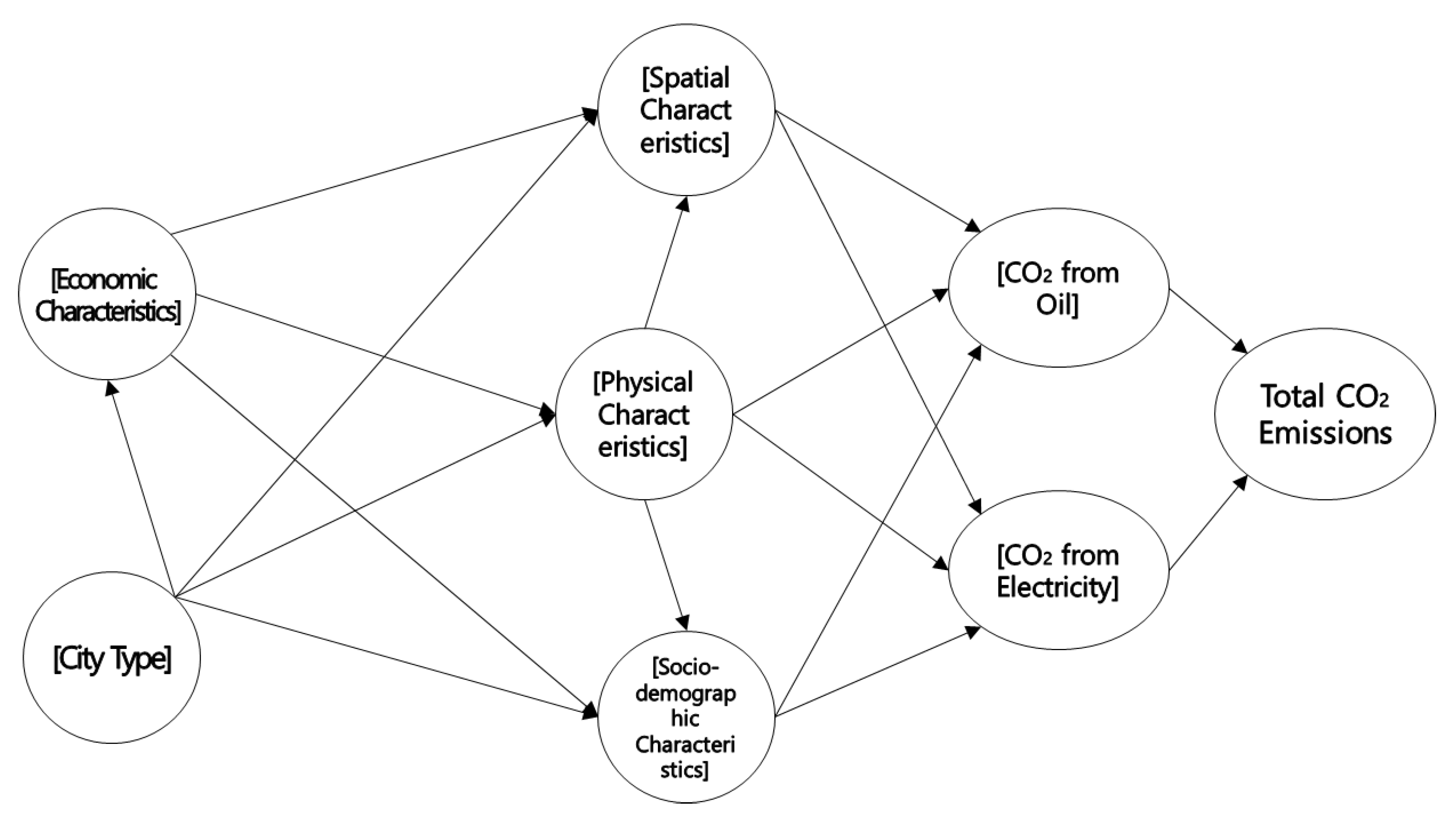
3.3. Total Impacts of Urban Development Intensity Characteristics that Affect CO₂ Emissions

Based on the analysis shown above, the total impacts (i.e., the sum of the direct and indirect impacts) of the UDI characteristics that affect CO₂ emissions from oil and electricity are shown in

Table 8. Comparison of the influence of UDI characteristics on the direct and indirect impacts.

Classification		Physical Characteristics	Spatial Characteristics	Socio-Demographic Characteristics	Economic Characteristics	City Type
Oil	Direct Impact	0.444 ***	−0.720 ***	−0.645 ***	-	-
	Indirect Impact	0.178 ***	-	-	−0.136	0.485 ***
	Total Impact	0.623 ***	−0.720 ***	−0.645 ***	−0.136	0.485 ***
Electricity	Direct Impact	0.630 ***	−0.242 ***	−0.747 ***	-	-
	Indirect Impact	0.109 ***	-	-	−0.048	0.118 ***
	Total Impact	0.739 ***	−0.242 ***	−0.747 ***	−0.048	0.118 ***

*** p < 0.01.

. Note that, because the total impact of a given UDI characteristic includes indirect impacts, the total impact varies considerably depending on the energy source. In other words, the impacts of oil and electricity may become smaller or larger.

These results support our hypothesis that physical, spatial, and socio–demographic characteristics directly affect CO₂ emissions from oil and electricity, while city type and economic characteristics indirectly affect CO₂ emissions through other characteristics (see Figure 3). Furthermore, the regression equations are shown in order to determine whether the given relationships are positive or negative and enable comparison with the results of previous studies.

Direct relationships can be represented as:

$$P{C}_i=0.29\left(number of vehicle{s}_i\right)+0.27\left(total length of road{s}_i\right)+0.42\left(number of housing unit{s}_i\right)-0.34\left(number of households using buse{s}_i\right),$$

(1)

$$S{C}_i=0.725\left(apartment residency rati{o}_i\right)+0.387\left(populationdensit{y}_i\right),$$

(2)

$$SD{C}_i=senior population rati{o}_i;$$

(3)

and indirect relationships can be represented as:

$$P{C}_i=-0.25(E{C}_i)+0.64(C{T}_i)+e_1,$$

(4)

$$S{C}_i=-0.17(P{C}_i)+0.19(E{C}_i)-0.59(C{T}_i)+e_1,$$

(5)

$$SD{C}_i=-0.25(E{C}_i)+0.73(C{T}_i)-0.08(P{C}_i)+e_1,$$

(6)

$$E{C}_i=0.793(financial self reliance rati{o}_i)+0.366\left(employmentnumbe{r}_i\right),$$

(7)

$$E{C}_i=-0.91(C{T}_i)+e_1,$$

(8)

$$C{T}_i=-0.234(P{C}_i)+0.201\left(S{C}_i\right)-0.304\left(E{C}_i\right)+0.447\left(SD{C}_i\right)+e_1;$$

(9)

and total relationships can be represented as:

$$O{E}_i=0.62(P{C}_i)-0.72(S{C}_i)-0.64(SD{C}_i)-0.13(E{C}_i)+0.48\left(C{T}_i\right)+e_1,$$

(10)

$$E{E}_i=0.73(P{C}_i)-0.24(S{C}_i)-0.74(SD{C}_i)-0.04(E{C}_i)+0.11\left(C{T}_i\right)+e_1,$$

(11)

where i = 107 cities, e₁ = error term, OE = CO₂ emissions from Oil, EE = CO₂ emissions from electricity, SCs = spatial characteristics, PCs = physical characteristics, SDCs = socio-demographic characteristics, ECs = economic characteristics, and CT = city type.

4. Discussion

Physical characteristics (PC) values become larger with higher numbers of vehicles, total road length, and numbers of houses, whereas PC values decrease with a higher number of public transportation users (see Equation (1)). Areas with large PC values can be characterized as vehicle-centric and having a high number of personally owned houses; these qualities increase CO₂ emissions (see Equations (10) and (11)). These results are similar to those found in previous studies regarding the relationships between automobiles and oil [15,32], road area and oil [6,33], and the number of housing units and electric energy consumption [34]. Moreover, the number of households using public transportation is related to transportation energy consumption. An increase in the number of households using public transportation helps reduce oil energy consumption, as it decreases overall vehicle use [15,32,35]. PC also indirectly affects CO₂ emissions via SCs (see Equation (5)) and socio–demographic characteristics (SDCs) (see Equation (6)).

Spatial characteristics (SC) values become larger with higher population densities and apartment residency ratios (see Equation (2)). Areas with large SC values can be characterized as developed with high spatial density, which decreases CO₂ emissions (see Equations (10) and (11)). These results support earlier claims that high-density development reduces CO₂ emissions [18,19,20].

SDCs increase with higher senior population ratios (see Equation (3). The SDC category includes only one measurement variable: the senior population ratio. Areas with large SDC values feature high senior population ratios and reduced CO₂ emissions, according to the formulas herein (see Equations (9) and (10)). However, these results contradict previous studies that state that energy consumption increases because elderly people spend more time in the home than other age groups [8,16]. This may show that the energy consumption patterns for elderly people in Korea differ from those in other countries. Specifically, the poverty rate of the elderly in Korea is 45.11%, which is the highest among OECD countries [57]. Considering that the next highest rate is 30.6%, the economic difficulties of the elderly in Korea are relatively large; it is possible that the elderly cannot afford adequate heating, and, thus, energy use decreases despite increasing amounts of time spent at home [58]. Meanwhile, CO₂ emission reduction strategies based on socio–demographic characteristics may be faster and more effective because SDCs have both large direct effects on CO₂ emissions via oil and electricity (−0.654 and −0.747, respectively) and smaller effects on other characteristics. However, there is no realistic policy to encourage the proportion of the elderly population per local government to reduce CO₂ emissions. Indirect plans and policies should be considered. To maintain low CO₂ emissions as the lives of the elderly improve, there are plans to increase support spaces such as senior citizen community centers and urban regeneration centered on energy efficiency improvement projects, and energy poverty reduction plans.

Economic characteristics (EC) values increase with higher rates of financial independence and numbers of employers (see Equation (6)). Large EC values decrease CO₂ emissions, but the coefficients are small and not statistically significant. ECs have a lower impact on oil and electricity CO₂ emissions compared to other characteristics, at −0.136 and −0.048, respectively (see Equations (10) and (11)). However, these results do not necessarily mean that ECs do not have significant effects on CO₂ emissions, as ECs’ indirect impacts may either increase or reduce emissions. Economic characteristics exhibit a positive (+) relationship with spatial characteristics that directly affects CO₂ emissions (see Equation (5)), but, conversely, exhibit negative (−) relationships with physical characteristics and socio–demographic characteristics (see Equations (4) and (6)). In other words, continuous economic growth directly increases CO₂ emissions but also has indirect reduction effects. These results contrast with the findings of Wang et al. [7].

The city type (CT) may be characterized as either medium or small (see Equation (9)). Like EC, CT also causes both increases and reductions in CO₂ emissions. According to Glaeser and Kahn [23], large cities are more efficient than medium and small cities in terms of per capita CO₂ emissions. Also, depending on the size of the city, CO₂ emissions are different for each energy source. In medium and small cities, oil CO₂ emissions are three times larger than the total CO₂ emissions from electricity generation (see Equations (10) and (11)). However, there is a positive effect on SCs as a city grows from small or medium to large, a negative effect on PCs (which reduce CO₂ emissions), and a negative effect on SDCs (which increase CO₂ emissions). Clearly, because the sign of the effect differs with the specific domain, emission reduction strategies must be appropriate to the development intensity characteristics in the given area; this result agrees with those from (Heinonen and Junnila [59]).

The results of this study verify the claims of previous research and emphasize the need for integrated urban policies for energy consumption reduction.

5. Conclusions

Studies relating to UDI are increasing with increased interest in the effects of UDI on CO₂ emissions. However, from an urban planning perspective, attempts to investigate the direct and indirect effects of the various UDI characteristics on CO₂ emissions and the interrelationships between those effects have been insufficient. This study investigates factors arising from UDI characteristics in Korea, calculates CO₂ emissions, and uses a structural equation model to analyze the interrelationships between emission impact factors. The analytical results and implications thereof are described below.

First, we identified UDI characteristics and factors that affect CO₂ emissions. Physical characteristics, spatial characteristics, and socio-demographic characteristics directly affect CO₂ emissions, while physical characteristics, economic characteristics, and city type indirectly affect CO₂ emissions; other characteristics have mediated effects. Among the factors analyzed, increasing the number of households that use public transportation, population density, apartment residency ratio, rate of financial independence, number of employers, and senior population ratio serves to reduce per capita CO₂ emissions, while increasing the number of cars, total road length, and number of housing units increases per capita CO₂ emissions.

Second, we compared our results with those from existing studies. Higher values of physical characteristics cause increases in CO₂ emissions, which is consistent with the results of most existing research. Higher values of spatial characteristics reduce CO₂ emissions. In other words, these results support existing studies in stating that dense cities reduce CO₂ emissions. On the other hand, economic characteristics have an impact on the total CO₂ emissions, since they affect other characteristics in both positive and negative ways. In other words, the results agree with the notion that continuous economic growth inevitably increases CO₂ emissions directly but can also lead to indirect reductions in certain areas. Socio–demographic characteristics results are not consistent with the results of existing research, as an increase in SDC values reduces CO₂ emissions. This suggests that the energy consumption patterns of certain groups affected by economic and other characteristics may differ by region and country. As to city type, medium and small cities have higher per capita CO₂ emissions than do large cities.

Lastly, the following urban planning strategies for CO₂ emissions were developed based on the results and discussion presented herein. The government should continually execute strategies to control factors that increase CO₂ emissions. In other words, future plans should discourage the construction of infrastructure such as personal houses, vehicles, and roads and instead encourage the use of public transportation. Strategies that promote city density are three times more effective for the reduction of CO₂ emissions from oil than for those from electricity. Accordingly, it is necessary to establish a plan that connects physical infrastructure, expands Transit Oriented Development–centered urban space structure development, apartments, and public facilities and makes public transportation more convenient. Because socio–demographic planning elements, such as certain groups of people, have little connection with industrial infrastructure, changes in these factors may effectively decrease CO₂ emissions at comparatively low cost; for example, home improvement projects for the elderly and high-efficiency electricity dissemination are effective CO₂ emissions reduction strategies. CO₂ emissions from the different energy sources vary with city size. In medium and small cities, the total effect on CO₂ emissions from oil is three times larger than the total effect on CO₂ emissions from electrical power. Accordingly, policies that strengthen urban infrastructure, promoting density and green transportation options, should be established in order to reduce oil consumption in medium and small cities. In large cities, green city development policies should be established.

This study reveals the direct and indirect relationships between UDI characteristics and CO₂ emissions and emphasizes the necessity of research on urban policy packages during urban planning for CO₂ reduction.

References

1. Watson, R.T.; Albritton, D.L. Climate Change 2001: Synthesis Report: Third Assessment Report of the Intergovernmental Panel on Climate Change; Cambridge University Press: Cambridge, UK, 2001. [Google Scholar]
2. Oliver, J.; Janssens-Maenhout, G.; Peters, J.; Wilson, J. Longterm Trend in Global CO2 Emissions; PBL Netherlands Environmental Assessment Agency: The Hague, The Netherlands, 2011. [Google Scholar]
3. Zhang, X.-H.; Zhang, R.; Wu, L.-Q.; Deng, S.-H.; Lin, L.-L.; Yu, X.-Y. The interactions among China’s economic growth and its energy consumption and emissions during 1978–2007. Ecol. Indic. 2013, 24, 83–95. [Google Scholar] [CrossRef]
4. Ou, J.; Liu, X.; Li, X.; Chen, Y. Quantifying the relationship between urban forms and carbon emissions using panel data analysis. Landsc. Ecol. 2013, 28, 1889–1907. [Google Scholar] [CrossRef]
5. Gordon, P.; Richardson, H.W. Gasoline consumption and cities: A reply. J. Am. Plan. Assoc. 1989, 55, 342–346. [Google Scholar] [CrossRef]
6. Newman, P.W.; Kenworthy, J.R. Gasoline consumption and cities: A comparison of US cities with a global survey. J. Am. Plan. Assoc. 1989, 55, 24–37. [Google Scholar] [CrossRef]
7. Wang, S.; Fang, C.; Wang, Y.; Huang, Y.; Ma, H. Quantifying the relationship between urban development intensity and carbon dioxide emissions using a panel data analysis. Ecol. Indic. 2015, 49, 121–131. [Google Scholar] [CrossRef]
8. Guerin, D.A.; Yust, B.L.; Coopet, J.G. Occupant predictors of household energy behavior and consumption change as found in energy studies since 1975. Fam. Consum. Sci. Res. J. 2000, 29, 48–80. [Google Scholar] [CrossRef]
9. Brownstone, D.; Golob, T.F. The impact of residential density on vehicle usage and energy consumption. J. Urban Econ. 2009, 65, 91–98. [Google Scholar] [CrossRef] [Green Version]
10. Tate, C.M.; Cuffney, T.F.; McMahon, G.; Giddings, E.M.; Coles, J.F.; Zappia, H. Use of an Urban Intensity Index to Assess Urban Effects on Streams in Three Contrasting Environmental Settings. Am. Fish. Soc. Symp. 2005, 47, 291–315. [Google Scholar]
11. Mendes, H.C. Measuring Urban Development Intensity: Is It Possible to Get an X-ray of Our Cities? Case Study: Tulsa, OK; The University of Oklahoma: Norman, OK, USA, 2008. [Google Scholar]
12. Talbi, B. CO2 emissions reduction in road transport sector in Tunisia. Renew. Sustain. Energy Rev. 2017, 69, 232–238. [Google Scholar] [CrossRef]
13. Schipper, L.; Bartlett, S.; Hawk, D.; Vine, E. Linking life-styles and energy use: A matter of time? Ann. Rev. Energy 1989, 14, 273–320. [Google Scholar] [CrossRef]
14. Fragkias, M.; Lobo, J.; Strumsky, D.; Seto, K.C. Does size matter? Scaling of CO2 emissions and US urban areas. PLoS ONE 2013, 8, e64727. [Google Scholar] [CrossRef] [PubMed]
15. Liu, C.; Shen, Q. An empirical analysis of the influence of urban form on household travel and energy consumption. Comput. Environ. Urban Syst. 2011, 35, 347–357. [Google Scholar] [CrossRef]
16. O’neill, B.C.; Chen, B.S. Demographic determinants of household energy use in the United States. Popul. Dev. Rev. 2002, 28, 53–88. [Google Scholar]
17. Fong, W.-K.; Matsumoto, H.; Lun, Y.-F.; Kimura, R. Influences of indirect lifestyle aspects and climate on household energy consumption. J. Asian Archit. Build. Eng. 2007, 6, 395–402. [Google Scholar] [CrossRef]
18. Anderson, W.P.; Kanaroglou, P.S.; Miller, E.J. Urban form, energy and the environment: A review of issues, evidence and policy. Urban Stud. 1996, 33, 7–35. [Google Scholar] [CrossRef]
19. Banister, D.; Watson, S.; Wood, C. Sustainable cities: Transport, energy, and urban form. Environ. Plan. B Plan. Des. 1997, 24, 125–143. [Google Scholar] [CrossRef]
20. Dhakal, S. Urban energy use and carbon emissions from cities in China and policy implications. Energy Policy 2009, 37, 4208–4219. [Google Scholar] [CrossRef]
21. Jenks, M.; Burgess, R. Compact Cities: Sustainable Urban Forms for Developing Countries; Taylor & Francis: Abingdon, UK, 2000. [Google Scholar]
22. Chiu, R.L. Social equity in housing in the Hong Kong special administrative region: A social sustainability perspective. Sustain. Dev. 2002, 10, 155–162. [Google Scholar] [CrossRef]
23. Glaeser, E.L.; Kahn, M.E. The greenness of cities: Carbon dioxide emissions and urban development. J. Urban Econ. 2010, 67, 404–418. [Google Scholar] [CrossRef] [Green Version]
24. Hillier, B. Space Is the Machine: A Configurational Theory of Architecture; Space Syntax: London, UK, 2007. [Google Scholar]
25. Parr, J.B. The regional economy, spatial structure and regional urban systems. Reg. Stud. 2014, 48, 1926–1938. [Google Scholar] [CrossRef]
26. Farber, S.; Li, X. Urban sprawl and social interaction potential: An empirical analysis of large metropolitan regions in the United States. J. Transp. Geogr. 2013, 31, 267–277. [Google Scholar] [CrossRef]
27. Bourne, L.S. Urban spatial structure: An introductory essay on concepts and criteria. In Internal Structure of the City; Oxford University Press: New York, NY, USA, 1982; Volume 45. [Google Scholar]
28. Antonescu, D.; Ghisa-Silea, M. Cities and their place in the European Union urban policy. Romanian J. Econ. Forecast. 2007, 4, 57–68. [Google Scholar]
29. Snyder, J.C.; Catanese, A.J. Introduction to Urban Planning; McGraw-Hill: New York, NY, USA, 1979. [Google Scholar]
30. Kaiser, E.J.; Godschalk, D.R.; Chapin, F.S. Urban Land Use Planning; University of Illinois Press: Urbana, IL, USA, 1995; Volume 4. [Google Scholar]
31. Foley, D.L. An approach to metropolitan spatial structure. In Explorations into Urban Structure; University of Pennsylvania Press: Philadelphia, PA, USA, 1964; pp. 21–78. [Google Scholar]
32. Lin, J.-J.; Yang, A.-T. Structural analysis of how urban form impacts travel demand: Evidence from Taipei. Urban Stud. 2009, 46, 1951–1967. [Google Scholar] [CrossRef]
33. Reckien, D.; Ewald, M.; Edenhofer, O.; Liideke, M.K. What parameters influence the spatial variations in CO2 emissions from road traffic in Berlin? Implications for urban planning to reduce anthropogenic CO2 emissions. Urban Stud. 2007, 44, 339–355. [Google Scholar] [CrossRef]
34. Steemers, K.; Yun, G.Y. Household energy consumption: A study of the role of occupants. Build. Res. Inf. 2009, 37, 625–637. [Google Scholar] [CrossRef]
35. Cervero, R.; Murakami, J. Effects of built environments on vehicle miles traveled: Evidence from 370 US urbanized areas. Environ. Plan. A 2010, 42, 400–418. [Google Scholar] [CrossRef]
36. Liao, C.-H.; Chang, C.-L.; Su, C.-Y.; Chiueh, P.-T. Correlation between land-use change and greenhouse gas emissions in urban areas. Int. J. Environ. Sci. Technol. 2013, 10, 1275–1286. [Google Scholar] [CrossRef] [Green Version]
37. Wang, Y.; Hayashi, Y.; Chen, J.; Li, Q. Changing urban form and transport CO2 emissions: An empirical analysis of Beijing, China. Sustainability 2014, 6, 4558–4579. [Google Scholar] [CrossRef]
38. Liu, X.; Sweeney, J. Modelling the impact of urban form on household energy demand and related CO2 emissions in the greater Dublin region. Energy Policy 2012, 46, 359–369. [Google Scholar] [CrossRef]
39. Hankey, S.; Marshall, J.D. Impacts of urban form on future US passenger-vehicle greenhouse gas emissions. Energy Policy 2010, 38, 4880–4887. [Google Scholar] [CrossRef]
40. Poumanyvong, P.; Kaneko, S. Does urbanization lead to less energy use and lower CO2 emissions? A cross-country analysis. Ecol. Econ. 2010, 70, 434–444. [Google Scholar] [CrossRef]
41. Kyoung Yong, K.; Young Ook, K. A study on the lead-lag effect of spatial configuration and economic activity—Focused on the change of street network structure and employment density. J. Korea Plan. Assoc. 2015, 50, 43–58. [Google Scholar]
42. Rossiter, J.R. The C-OAR-SE procedure for scale development in marketing. Int. J. Res. Mark. 2002, 19, 305–335. [Google Scholar] [CrossRef] [Green Version]
43. Jarvis, C.B.; MacKenzie, S.B.; Podsakoff, P.M. A critical review of construct indicators and measurement model misspecification in marketing and consumer research. J. Consum. Res. 2003, 30, 199–218. [Google Scholar] [CrossRef]
44. Götz, O.; Liehr-Gobbers, K.; Krafft, M. Evaluation of structural equation models using the partial least squares (PLS) approach. In Handbook of Partial Least Squares; Springer: London, UK, 2010; pp. 691–711. [Google Scholar]
45. Peng, D.X.; Lai, F. Using partial least squares in operations management research: A practical guideline and summary of past research. J. Oper. Manag. 2012, 30, 467–480. [Google Scholar] [CrossRef]
46. Henseler, J.; Hubona, G.; Ray, P.A. Using PLS path modeling in new technology research: Updated guidelines. Ind. Manag. Data Syst. 2016, 116, 2–20. [Google Scholar] [CrossRef]
47. Chin, W.W. Bootstrap cross-validation indices for PLS path model assessment. In Handbook of Partial Least Squares; Springer: London, UK, 2010; pp. 83–97. [Google Scholar]
48. Roldán, J.L.; Sánchez-Franco, M.J. Variance-based structural equation modeling: Guidelines for using partial least squares. In Research Methodologies, Innovations and Philosophies in Software Systems Engineering and Information Systems; Information Science Reference: Hershey, PA, USA, 2012; Volume 193. [Google Scholar]
49. Barroso, A.; González-López, Ó.R.; Sanguino, R.; Buenadicha-Mateos, M. Analysis and evaluation of the largest 500 family firms’ websites through PLS-SEM technique. Sustainability 2018, 10, 557. [Google Scholar] [CrossRef]
50. Fornell, C.; Larcker, D.F. Evaluating structural equation models with unobservable variables and measurement error. J. Mark. Res. 1981, 18, 39–50. [Google Scholar] [CrossRef]
51. Hair, J.F., Jr.; Hult, G.T.M.; Ringle, C.; Sarstedt, M. A Primer on Partial Least Squares Structural Equation Modeling (PLS-SEM); Sage Publications: Thousand Oaks, CA, USA, 2016. [Google Scholar]
52. Andreev, P.; Heart, T.; Maoz, H.; Pliskin, N. Validating formative partial least squares (PLS) models: Methodological review and empirical illustration. In Proceedings of the 13th International Conference on Information Systems, Phoenix, AZ, USA, 15–18 December 2009; AIS Electronic Library: San Francisco, CA, USA, 2009; p. 193. [Google Scholar]
53. Hassan, S.H.; Ramayah, T.; Mohamed, O.; Maghsoudi, A. E-lifestyle, customer satisfaction, and loyalty among the generation Y mobile users. Asian Soc. Sci. 2015, 11, 157. [Google Scholar] [CrossRef]
54. Chin, W.W. Commentary: Issues and Opinion on Structural Equation Modeling; JSTOR: New York, NY, USA, 1998. [Google Scholar]
55. Tenenhaus, M.; Pages, J.; Ambroisine, L.; Guinot, C. PLS methodology to study relationships between hedonic judgements and product characteristics. Food Qual. Preference 2005, 16, 315–325. [Google Scholar] [CrossRef]
56. Temme, D.; Kreis, H.; Hildebrandt, L. PLS Path Modeling: A Software Review; Humboldt University of Berlin: Berlin, Germany, 2006. [Google Scholar]
57. OECD. Pensions at a Glance 2011: Retirement-Income Systems in OECD and G20 Countries; Organisation for Economic Co-operation and Development (OECD) Publishing: Paris, France, 2011. [Google Scholar]
58. Hyeongyeong, K. The actual state of energy poverty and its political implications. Health Welf. Issue Focus 2015, 281, 1–8. [Google Scholar]
59. Heinonen, J.; Junnila, S. A carbon consumption comparison of rural and urban lifestyles. Sustainability 2011, 3, 1234–1249. [Google Scholar] [CrossRef]
Figure 1. Suggested model.
Sustainability 10 01838 g001
Figure 2. CO2 emissions from oil and electricity.
Sustainability 10 01838 g002
Figure 3. Impact structure model results showing the effects of UDI characteristics on CO2 emissions.
Sustainability 10 01838 g003