Article

A Multi-Temporal Analyses of Land Surface Temperature Using Landsat-8 Data and Open Source Software: The Case Study of Modena, Italy

Department of Engineering “Enzo Ferrari”, University of Modena and Reggio Emilia, Via Vivarelli 10, 41125 Modena, Italy
*
Author to whom correspondence should be addressed.
Sustainability 2018, 10(5), 1678; https://doi.org/10.3390/su10051678
Submission received: 26 April 2018 / Revised: 17 May 2018 / Accepted: 18 May 2018 / Published: 22 May 2018

Abstract

:
The Urban Heat Island (UHI) phenomenon, namely urban areas where the atmospheric temperature is significantly higher than in the surrounding rural areas, is currently a very well-known topic both in the scientific community and in public debates. Growing urbanization is one of the anthropic causes of UHI. The UHI phenomenon has a negative impact on the life quality of the local population (thermal discomfort, summer thermal shock, etc.), thus investigations and analyses on this topic are really useful and important for correct and sustainable urban planning; this study is included in this context. A multi-temporal analysis was performed in the municipality of Modena (Italy) to identify and estimate the Surface Urban Heat Island (SUHI, strictly correlated to the UHI phenomenon) from 2014 to 2017. For this purpose, Landsat-8 satellite images were processed with Quantum Geographic Information System (QGIS) to obtain the Land Surface Temperature (LST) and the Normalized Difference Vegetation Index (NDVI). For every pixel, LST and NDVI values of three regions of interest (ROI, i.e., Countryside, Suburbs, and City Center) were extracted and their correlations were investigated. A maximum variation of 6.4 °C in the LST values between City Center and Countryside was highlighted, confirming the presence of the SUHI phenomenon even in a medium-sized municipality like Modena. The implemented procedure demonstrates that satellite data are suitable for SUHI identification and estimation, therefore it could be a useful tool for public administration for urban planning policies.

1. Background

About half of the world population lives in urban areas [1]. The global urbanization rate is expected to increase by 70% compared to the current world population [2], both because of the continued emergence of new urban areas [3] and because of the constant population migration from rural to urban and suburban areas [4,5]. It is not therefore surprising that the negative impacts of urbanization are an ever-growing global concern [6,7,8,9,10]. Urbanization has a negative impact on the environment, mainly due to pollution, changes in the physical and chemical properties of the atmosphere, and in the type of cover of the soil surface [11]. These phenomena lead to so-called Urban Heat Islands (UHI), namely urban areas where the atmospheric temperature is significantly higher than that in the surrounding rural areas [12]. The presence of UHIs is an increasing phenomenon studied by the international scientific community because of its dangerous and significant effects. In fact, the temperature increase has effects on the environment (higher temperatures cause higher energy consumption, photochemical smog, and worsening of the air quality), on the climate and on human health [13,14,15,16].
Concerning urban planning policies, nowadays, public administrations have to take into account not only socioeconomic perspectives but also environmental sustainability [17]. Obviously, the UHI phenomenon is also a topic that has to be considered in administration decisions because it negatively influences population life quality. It leads to thermal discomfort and thermal shock, especially during the hot seasons [18,19]. The presence of UHI is typical of highly urbanized areas, but there is currently a progressive increase of this phenomenon not only for metropolises but also for medium-sized municipalities.
The main objective of this study is to investigate the presence, extent, and intensity of Surface Urban Heat Islands (SUHIs) in the municipality of Modena through the use of remote sensing images. Environmental remote sensing is a very useful tool to analyze this phenomenon by calculating the Land Surface Temperature (LST); this is why this study deals with SUHI instead of UHI [20,21,22,23,24,25]. The trend of the LST and the SUHI intensity are highly correlated—an increase of 0.1 °C of the urban LST compared to the rural LST corresponds to an increase of 0.04 °C of SUHI intensity [26]. This result, however, is retrieved only in the Mediterranean area, due to the specific characteristics of the cities of this region, which may not be found in other parts of the world.
Also, SUHI and UHI phenomena are strictly correlated and in particular the SUHI represents an indirect estimate of the UHI [27,28]. In scientific literature, a variety of studies have combined LST, usually used for the SUHI phenomenon, and air temperature data, usually used for the UHI phenomenon [29,30,31,32,33].
Some preliminary assessments on the study area are mandatory to understand and analyze results. First of all, Modena has different characteristics from the American cities that are usually used to define the UHI phenomenon [34]. Modena is a medium-sized municipality, without a high urban density and with a surrounding countryside with a lot of little villages. Instead, American metropolises usually have a very high urban density and the surrounding areas are empty. For these reasons, the difference of temperatures between cities and the countryside are not as high as in other studies in scientific literature dealing with bigger cities.
Furthermore, Modena has many well-distributed green areas that contribute to reduce the UHI phenomenon and to mitigate the temperatures in the areas that have a high urban density. Indeed, green areas are one of the most common strategies used to mitigate UHIs [17,35,36,37,38].
The city of Modena therefore represents a different area from those usually studied for the analysis of the SUHI phenomenon in the existing scientific literature. In the current state of the art, in fact, it is possible to find numerous studies on UHI related to large cities [39] both in America and in Asia [40,41]. In the Mediterranean area there are many studies focused on large cities such as Barcelona [42], Athens [43,44], Salonicco [45], and Tel Aviv [46]. In Italy, numerous studies considered the UHI of Rome or Milan [47,48,49,50], while recently other studies have been implemented on cities like Bologna [51], Padua [52], and Venice [53]. Concerning the southern part of Italy, currently there is only one study that reports an analysis of the LST of the major southern cities (Bari, Naples, Palermo, and Catania) [54]. In this study, the LST value of the rural area is not present, thus it is not possible to quantify the SUHI.
For the city of Modena, some considerations of the UHI phenomenon have been carried out in the studies of Bonafè and Zauli Sajani [51,55]. Contrary to the methodology presented in this paper, these studies use ground station measurements for UHI intensity estimation. Furthermore, in Reference [51], not the entire area of Modena is considered but only specific districts.
No existing study in the scientific literature uses remote sensing data on a medium-sized city like Modena, placed in a highly polluted area (Po Valley), to identify and estimate SUHIs. In addition, there are only few studies that use Quantum Geographic Information System (QGIS) procedures (open source software) applied to remote sensing data for these purposes [56].
Another observation concerns the climate that has characterized the study area in the last two years. In this period, various climatic anomalies occurred as a consequence of the global climate change. In particular, winter was very humid with high temperatures and no snow. Also, summer was quite wet, especially in July and between the end of August and the beginning of September. These weather and climate conditions surely have an influence on the results obtained by remote sensing, because evapotranspiration influences the temperatures of urban and rural areas [57,58,59,60,61].
In this framework it is important to highlight that the municipality of Modena, in 2010, put in place a plan of action for sustainable energy (SEAP). This plan is included in the “good practices” for the European Green Infrastructure Strategies because it provides an increase in green infrastructures in agricultural areas, ecological zones, and public green. In particular, an increase in urban forest of 127.5 ha has been planned for implementation between 2011 and 2020 [62,63].
Thus, using the methodology developed in this paper, the city administrators will have a powerful tool to identify SUHIs and their intensity in different years. In this way, urban policies can be directed to those areas where the SUHI phenomenon is still present and creates discomfort in the population. Furthermore, the public administration could evaluate appropriate mitigation measures such as green roofs, cool materials, and green areas [64,65] that lead to a more sustainable life quality. In addition, using this methodology, it is possible to evaluate whether the policies entailed within the framework of the European Green Infrastructure Strategies are producing the desired results.

2. Materials and Methods

The analysis of the SUHI phenomenon in these areas was carried out using an experimental plugin for QGIS [66], called the Semi-Automatic Classification Plugin (SCP) [67], that allows use of the free open source software QGIS as a remote sensing software. With this plugin, temperature maps can be obtained from “raw” remote sensing images acquired by the Landsat-8 satellite sensor.
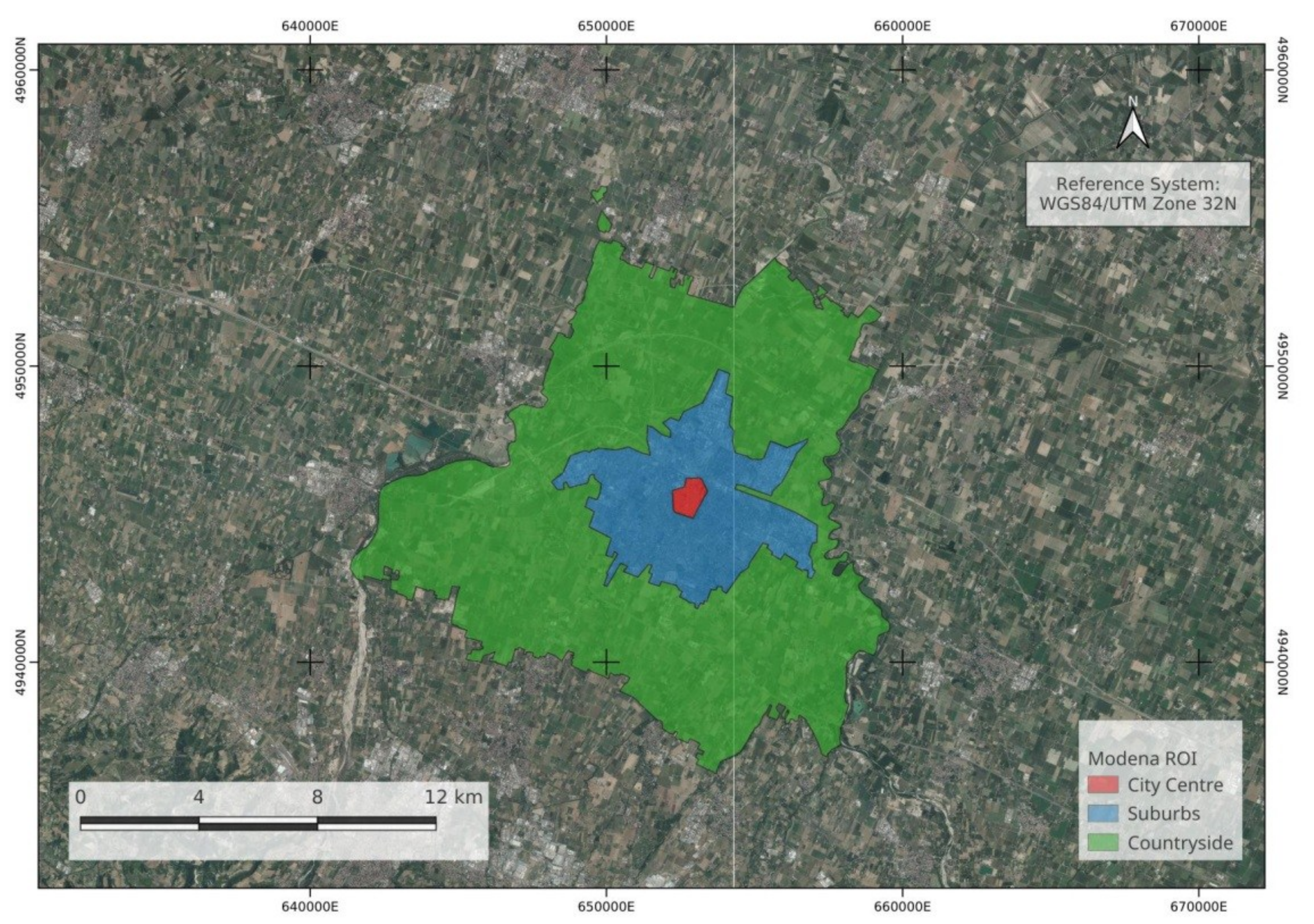
The study area includes the municipality of Modena located in the Emilia Romagna region, Italy. The environmental context is the Po Valley, which is characterized by a high population density and intensive agriculture. The LST was computed using the equation suggested by Weng [23]. Then, additional processing was conducted in order to create three Regions of Interest (ROI) within each image: the City Center region, the Suburbs region, and the Countryside region. For each ROI, LST maps and Normalized Difference Vegetation Index (NDVI) maps were retrieved. Creating these ROIs also allowed the estimation of the temperature difference between Countryside and City Center, and thus allowed us to correlate it with the SUHI phenomenon in the studied period (2014–2017) [68,69,70]. Finally, NDVI maps were used to analyze the correlation between land cover and LST maps.
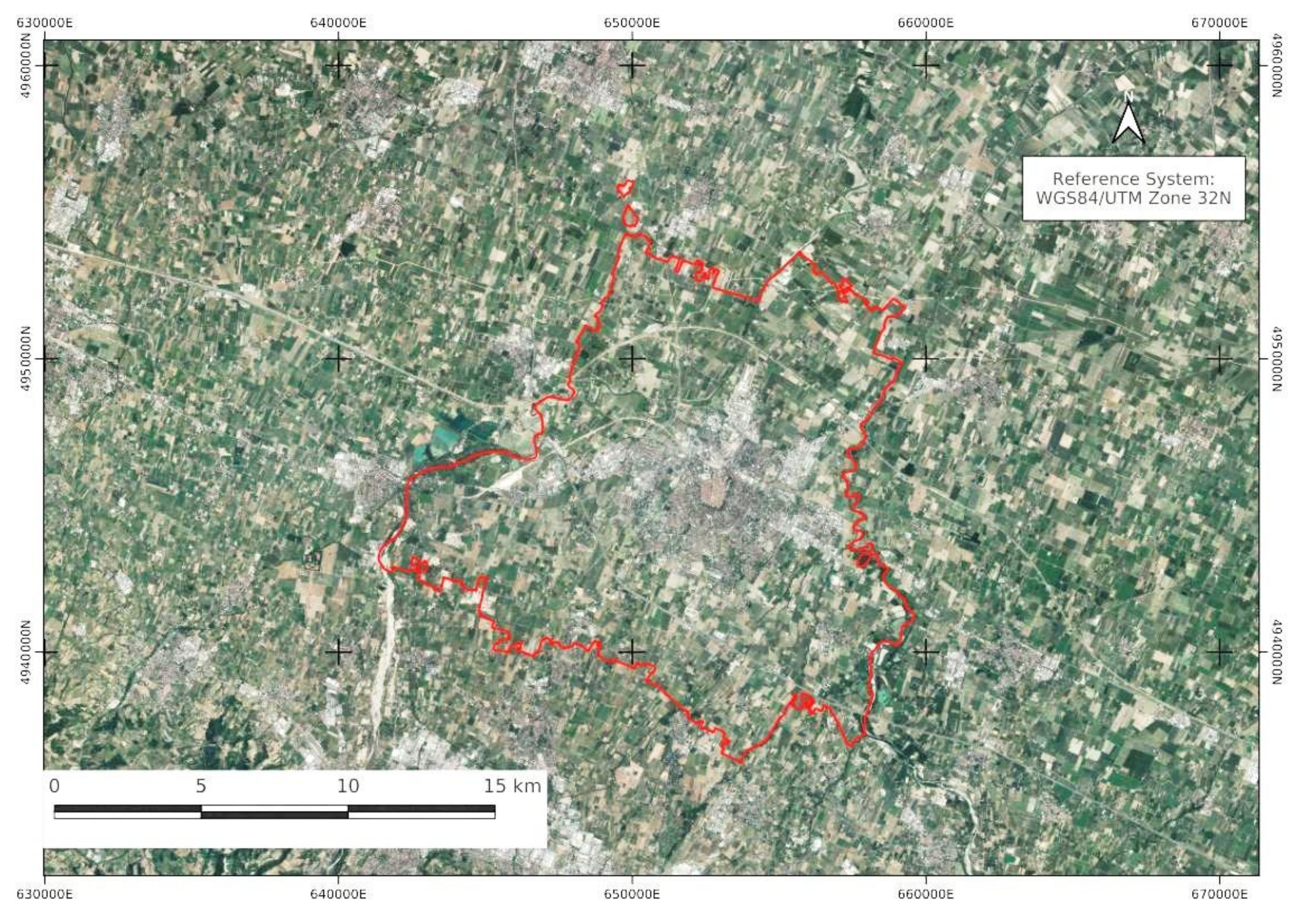
2.1. Study Area

The study area is the municipality of Modena, Italy (Figure 1). Modena has 184,826 inhabitants and an area of 183.19 km2 [
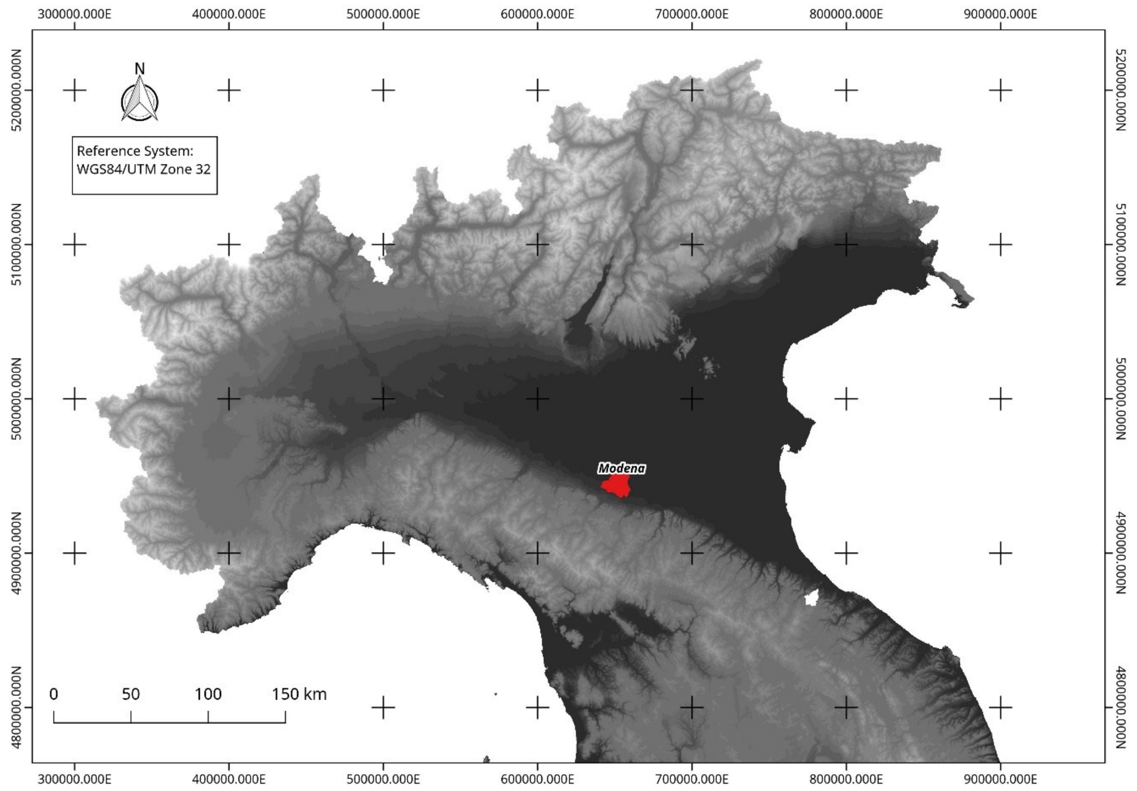
71]. Modena is located in the north of Italy, along the “via Aemilia”, an ancient Roman road running from Rimini to Piacenza on the river Po (Figure 2). The Po Valley is characterized by a high population density and by processes of industrialization and intensive agriculture (it is among the most productive agricultural areas within Europe) [72]. The climate of this region is partially continental: summers are hot with intense heat waves while winters are cold and wet, usually with atmospheric stability conditions and fog. Normally precipitation is concentrated during autumn and spring. Summer and winter are the driest seasons [57,58,72,73]. In order to have a clear climate situation of the study area, Table 1 reports some climate information. The data are divided into two series: an historical series from 1971–2000 and another time series from 2001 to 2017. For each series, Table 1 shows values of seasonal mean temperature, seasonal mean of the maximum daily temperatures, seasonal mean of the minimum daily temperatures, and seasonal mean of precipitation. The data referred to the City Center region were acquired by the Weather Station “Osservatorio Geofisico di Modena”, located in the urban area of Modena (Long: 10°55′47.2″ E, Lat: 44°38′52.9″ N) [74], while the data referred to the Countryside region were acquired by the ARPAE Weather Station of Albareto (Long: 10°57′24″ E, Lat: 44°42′7″ N). In Table 1, all temperature values of the historical series increase in the time series in every season. The increase of the values vary between 1.4 °C and 2 °C. Also, the values of precipitation increase in every season except summer. In Modena, starting from the 1980s, climate change has exhibited the same trend as the global climate change. The changes cause extreme events such as jumps in temperature or increases in the distribution and amount of precipitation [57].
The area of Modena was chosen as a first area of interest for the proposed methodology for its characteristics in terms of:
  • Dimensions. Modena is a medium-sized municipality and the scientific literature does not investigate SUHIs of these kind of cities with remote sensing data;
  • Climate situation;
  • Geographical position. Modena is located in one of the most industrialized areas of Europe, as well as one with the highest levels of air pollutants [75];
  • Active urban policies. Analyzing three years of data allowed us to investigate whether urban policies on green infrastructures are effective or not.
These characteristics render Modena an ideal test site for the developed methodology.

2.2. Landsat-8 Data

The Landsat-8 satellite was successfully launched on 11 February 2013 and deployed into orbit with two instruments on board: (1) the Operational Land Imager (OLI), whose spatial resolution is 30 m, with nine bands in the visible (VIS), the near infrared (NIR), and the short-wave infrared (SWIR) spectral regions; and (2) the Thermal Infrared Sensor (TIRS) with two spectral bands in the long-wave infrared (LWIR) region. The spatial resolution of TIRS data is 100 m with a revisit time of 16 days [75,76,77,78,79] (Table 2).
The data used for this study are the “raw” remote sensing images acquired from the Landsat-8 satellite sensors, provided free of charge by the United States Geological Survey (USGS) (Table 3).
Images were divided into three seasons depending on mean LST values retrieved by satellite data: hot season (LST > 30 °C); mid season (10 °C < LST < 30 °C); cold season (LST < 10 °C).
As reported in Table 3, there are 15 daily images covering about the hot, mid, and cold seasons of four years. The scene center time is about 10:00 UTC. Only images with a clear-sky condition were selected.
There are only two images from 2015 because of the cloud cover, but winter 2015 can be represented by the image taken on 12 December 2014. Autumn 2015 can be represented by the image taken on 10 September 2015, which presents typical autumnal climatic conditions. Therefore, the year 2015 can be considered completely covered, except for spring.
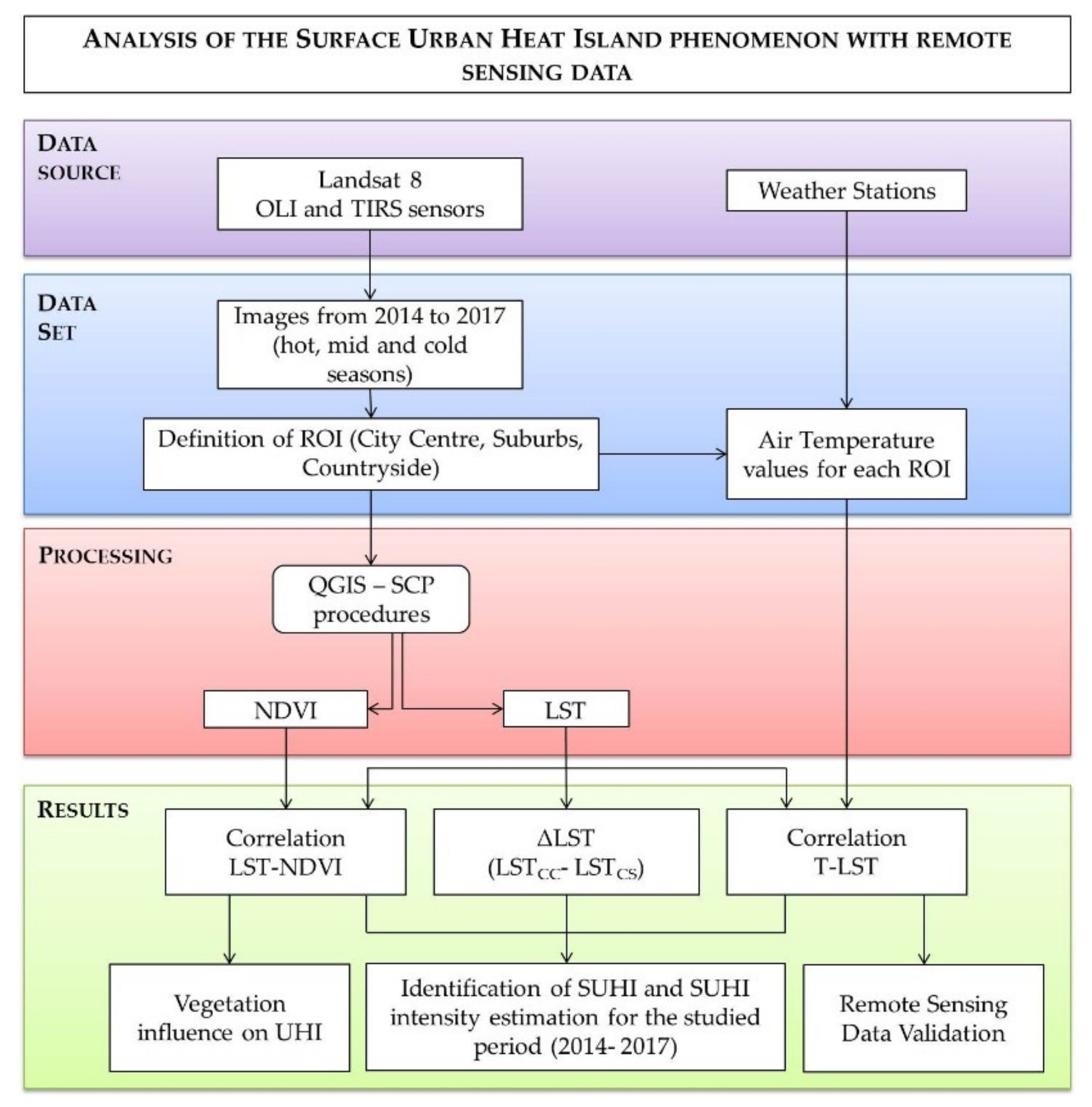
For the entire procedure, the Semi-Automatic Classification Plugin (SCP) on the open source software QGIS was used. The SCP plugin allows one to use remote sensing functions in QGIS [22,24,67]. The methodology, from input data to obtained results, is shown in the conceptual diagram in Figure 3. Each step is described in detail in the following subsections.

2.3. Data Processing

a. Conversion to Top of Atmosphere (TOA) Radiance
OLI and TIRS band data can be converted to top of atmosphere (TOA) spectral radiance using radiance rescaling factors provided in the metadata file [80]:
Lλ = ML × Qcal + AL
where:
  • Lλ = top of atmosphere spectral radiance (TOA) (W/(m2 srad μm)).
  • ML = band-specific multiplicative rescaling factor from the image metadata (W/(m2 srad μm)).
  • AL = band-specific additive rescaling factor from the image metadata (W/(m2 srad μm)).
  • Qcal = digital number (DN).
b. Conversion to TOA Reflectance
OLI band data were converted to TOA planetary reflectance using reflectance rescaling coefficients provided in the image metadata files [80]. The following equation is used to convert DN values to TOA reflectance for OLI data:
ρλ = Mρ × Qcal + Aρ
where:
  • ρλ = TOA reflectance.
  • Mρ = band-specific multiplicative rescaling factor from the metadata.
  • Aρ = band-specific additive rescaling factor from the metadata.
  • Qca = digital number.
c. Conversion to At-Satellite Brightness Temperature
TIRS band data were converted from spectral radiance to brightness temperature using the thermal constants provided in the image the metadata file [80]:
T = K2/ln ((K1/Lλ) + 1)
where:
  • T = at-satellite brightness temperature (K).
  • Lλ = TOA spectral radiance (W/(m2 srad μm)).
  • K1 = band-specific thermal conversion constant from the metadata (W/(m2 srad μm)).
  • K2 = band-specific thermal conversion constant from the metadata (K).
d. Clip of the image using the shapefile of Modena municipality, provided for free by the cartographic archive of the Emilia Romagna region (official website “Geoportale dell’Emilia Romagna”)
e. Calculation of Normalized Different Vegetation Index (NDVI)
This index is computed using spectral reflectance in the near infrared band and in the red band. It provides a rapid estimation of the presence of vegetation. NDVI values ranges from −1 to 1. Higher NDVI values indicate dense vegetation while lower values (typically from 0 to 0.2) identify light or dark soils [24]. NDVI is computed using the following equation:
NDVI = (ρNIR − ρRed)/(ρNIR + ρRed)
where:
  • ρNIR = near infrared band reflectance.
  • ρRED = red band reflectance.
f. Fractional Vegetation Cover (FVC)
NDVI was used to calculate FVC, an index that estimates the proportion of an area covered by a set of predefined type of vegetation or soil cover [24].
The following equation is used to calculate FVC:
FVC = (NDVI − NDVIs)/(NDVIv − NDVIs)
where:
  • NDVIs = NDVI value for bare soils.
  • NDVIv = NDVI value for fully vegetated soils.
The NDVIs value was set equal to 0.1, while the NDVIv value was set equal to 0.65 [22].
g. Calculation of Land Surface Emissivity (LSE), which is a measurement of the capacity of a material to radiate energy [24]
ε = (εs × (1 − FVC)) + (εv × FVC)
where:
  • εs = typical soil emissivity (0.93).
  • εv = typical vegetation emissivity (0.98).
h. Estimation of LST
LST can be calculated from the at-satellite brightness temperature TB [23]. LST was first computed in K, then converted to °C.
LST = TB/(1 + (λ × s × TB/c2) × ln(ε))
where:
  • λ = wavelength of the emitted radiance (11.5 μm for band 10 in Landsat-8 OLI).
  • c2 = h × c/s = 1.4388 × 10⁻² m K.
  • s = Boltzmann constant = 1.38 × 10⁻²³ J/K.
  • h = Planck’s constant = 6.626 × 10⁻³⁴ Js.
  • c = velocity of light = 2.998 × 10⁸ m/s.
  • ε = emissivity.

3. Results and Discussion

3.1. LST Maps

The methodology was applied to the dataset in order to obtain LST maps of Modena for different climate seasons. In this section only a few significant images are shown of the 15 processed. The statistical results on the next pages were, however, retrieved using all of the images listed in Table 3.
Figure 4 shows the LST map of the study area on 7 April 2014. The minimum value is 17.5 °C, the maximum value is 29 °C. Thanks to the spatial resolution of the TIRS sensor, inside the city in the industrial areas (LST values between 28 °C and 29 °C) it is possible to identify dense areas (most with LST values between 25.5 °C and 27.8 °C) and vegetation areas (LST values between 17.5 °C to 22 °C). Also, small residential areas and bare soils (LST values from 23 °C to 29 °C) could identified. Furthermore, main roads are clearly visible (LST values of about 23 °C). In the main urban area, LSTs are on average higher than in the countryside (the maximum temperature difference between the urban area and rural area is about 11 °C), confirming the presence of the SUHI phenomenon. In the following section, the difference between the urban LST and the rural LST will be further analyzed.
In winter, the LST maps show a more homogeneous distribution of temperatures and sometimes the urban LST values (from 0 °C to 2 °C) are slightly lower than the rural LST values (highly variable values that average between 0 °C and 5 °C). The map in Figure 5, for example, shows the study area on 9 January 2017. The situation is significantly different from that of Figure 4. LST values are very similar both in urban and in rural zones, thus in this period the SUHI phenomenon is not visible from this kind of data. In accordance with the scientific literature [61,81], during the winter period an inversion of temperature trends could occur (urban areas have lower temperatures than rural areas), especially in medium-sized municipalities like Modena. In order to explain this map, an investigation of the presence of water in the study area is required. When humidity levels are very high, the water evaporation and the plant transpiration saturate the atmosphere, thus countryside and city temperatures tend to flatten, out becoming much more similar to each other [61,81]. For this reason, in humid periods the SUHI is barely identifiable using remote sensing techniques, which however does not mean that the SUHI does not exist. For example, a temperature increase of just one or two degrees with humidity levels exceeding 90% does not allow the definition of the UHI phenomenon on an urban scale, but the population feels health discomforts nonetheless [82].

3.2. Region of Interest

To analyze temperature variations between urban areas and rural areas, three ROIs were created. A shapefile built thanks to municipality information was overlaid on each image in order to divide the municipality of Modena in three areas: City Center, Suburbs, and Countryside (Figure 6). These ROIs correspond to three specific Local Climate Zones (LCZs) defined by Stewart and Oke as “regions of uniform surfaces cover, structure, material, and human activity that span hundreds of meters to several kilometers in horizontal scale” [83]. City Center corresponds to LCZ1 (Compact Midrise) characterized by a building surface fraction between 40% and 70%. Suburbs corresponds to LCZ5 (Open Midrise) characterized by a building surface fraction between 20% and 40%. Countryside corresponds to LCZD (Low Plants) characterized by a building surface fraction less than 10% [83]. The building surface fraction represents the ratio of building plan area to total plan area (%). For Modena’s ROIs, the building surface fraction is equal to 46% for City Center, 20% for Suburbs, and 2% for Countryside. LCZs are defined in a univocal way based on specific parameters. The link between ROIs and LCZs allows the repeatability of the present methodology as well as comparison with other study areas.
Table 4 shows the average LST value of each ROI for every image and the difference (ΔLST) between the City Center LST values (LSTCC) and the Countryside LST values (LSTCS). These values allow to have a first evaluation of the intensity of the SUHI phenomenon. Suburbs LST values are not considered for this estimation because they are often very similar to City Center LST values.
Looking at Table 4, it can be observed that the images of cold seasons are usually associated with low LST variations (≤2 °C). Accordingly, with Figure 4 the SUHI phenomenon is not visible in these seasons with Landsat-8 data and thus it is not possible to correlate SUHIs with the UHI phenomenon.
Otherwise, images of hot seasons (spring and summer) are mostly associated with high LST variations (>2 °C). In this case it is possible to clearly identify the SUHI phenomenon and estimate its intensity. In Table 4 it is possible to observe the maximum and the minimum LST variation in the three seasons of interest. For the hot season, this value reached 6.4 °C, confirming the presence of the SUHI phenomenon and thus of the UHI phenomenon.
An exception of this analysis is represented by the image acquired on 9 January 2017. LST values for different regions are very close and the ΔLST between City Center and Countryside is lower than 2 °C. This anomaly is due to particular weather conditions of the days prior to the image acquisition; 2 and 3 July 2017 were in fact cloudy days with temperatures below the usual seasonal means.
Figure 7 shows a graphical representation of mean LST values for each acquired image and for each ROI—during hot seasons, the SUHI phenomenon is clearly visible.
For example, between April 2014 and October 2014, the difference between City Center LST values and Countryside LST values is clear, ranging from 3 °C and 5 °C. Similarly, from April 2015 to September 2015, the LST variation ranges from 1 °C to 5 °C (July 2015). From April 2016 to October 2016 and also from April 2017 to September 2017, this difference in LST values is not so remarkable, with ΔLST values ranging from 1 °C to 3 °C.
During cold seasons, the temperature lines in Figure 7 are almost completely overlapped, showing no SUHI presence. Thus, from October 2014 to March 2015, from October 2015 to April 2016, and from October 2016 to April 2017, LST values are very close for all three regions of interest.
In general, the LST peaks are higher in 2014–2015 and lower in 2016–2017. Winter 2017 had very low LST values compared to the other winters.
The results highlighted in Table 5 and visually shown in Figure 7 could be compared to scientific studies on UHI even if the present study deals with SUHI. In Asian large cities, the UHI intensity ranges from 0.4 to 11 °C. These values are largely influenced by the monsoon circulation [40]. In Europe, in particular in the Mediterranean area, it is possible to find UHI intensity values from 3 °C to 7 °C for cities like Athens and Salonicco [44,45]. Focusing on small cities, two interesting studies show the presence of UHI even in cities with less than 100,000 inhabitants [84,85]. These studies revealed a mean summer UHI intensity from 2.6 to 8 °C.
Table 6 show the UHI intensity retrieved for Italian cities in the scientific literature during the hot seasons. Even if these values are related to UHI and not to SUHI and these cities exhibit some differences from Modena (size, position, and inhabitants), it is possible to notice that the results obtained from this study are comparable with the values in Table 6. In particular, Zauli Sajani et al. [51] analyzed a large area that includes Bologna as well as Modena: the UHI intensity values measured by the meteorological station during the summer period are coherent with the results obtained from the methodology presented in this paper.
In Figure 7, the air temperature values are also reported. In particular, air temperature data for City Center and Countryside were retrieved from two weather stations provided by ARPAE Emilia Romagna, TCC and TCS, respectively.
These air temperature values are highly correlated to satellite LST values as it is possible to observe both in Figure 7 and Figure 8. The Pearson coefficients (r) shown in Figure 8 and in Table 7 have values closer to 1, which means there is an excellent correlation between LST values and air temperature values.
The results shown in Figure 8 are very important because they prove the effectiveness and reliability of satellite measurements for the study of SUHIs and consequently of UHIs. The high correlation with air temperatures measured by weather stations demonstrates that the methodology is repeatable and can be transferred to other areas similar to the city of Modena (medium-sized municipalities). In urban areas with different dimensions (large cities or small municipalities), the methodology can still be applied, only requiring the foresight to choose carefully the ROIs. In particular, the number and size of these regions must be appropriate to the study area. In this framework, the reference to LCZs [83] allows, for cities of different dimensions, the identification of the correct ROI number and size to study the SUHI phenomenon. Weather stations must also be chosen accurately as they are representative of the investigated ROI. Possible influences from traffic or emissions from industrial activities must be avoided if possible.

3.3. NDVI Maps

NDVI maps were retrieved in order to partially identify surface land cover and correlate it with LST values [87]. Figure 9 represents the NDVI map of the “Modena 7 April 2014” Landsat image. High values of NDVI (0.6 to 0.9) suggest a high density of vegetation, and low values of NDVI (from 0 to 0.3) suggest the presence of bare soil or artificial surfaces.
Obviously, urban areas present low NDVI values and rural areas have high NDVI values. From the NDVI map presented in Figure 9, it is possible to recognize built-up areas (or bare soil areas) and vegetation areas. NDVI maps are consistent with scientific literature data [28,88]. As reported by Yuan et al. [15], lower LSTs usually are found in areas with high NDVI. This negative correlation between NDVI and LST is valuable for urban climate studies. However, NDVI measurements are subject to seasonal variations, which may influence the results of SUHI studies.

3.4. LST-NDVI Correlation

For every pixel of the images from 7 April 2014, 15 July 2015, and 9 January 2017, the LST and NDVI values were extracted to make a correlation analysis.
Focusing on the image from 7 April 2014 and the image from 15 July 2015, Figure 10 shows that high values of NDVI correspond to low values of LST and vice versa. Thus, the presence of vegetation corresponds to lower LST values.
Regarding the 9 January 2017 image, it is difficult to make observations by just looking at the maps; it is necessary to analyze Table 8. This table reports the Pearson correlation coefficient between LST and NDVI computed for each ROI in the three images analyzed in Figure 10 (“Modena 7 April 2014”, “Modena 15 July 2015”, and “Modena 9 January 2017”).
For the images of April 2014 and July 2015, r values are close to 1, suggesting a strong correlation between NDVI and LST. Instead, for the image of January 2017, the r value is close to 0, thus a poor correlation between NDVI and LST is highlighted.
Compared to “Modena 7 April 2014” and to “Modena 15 July 2015”, the January 2017 image has two main differences: the low LST-NDVI correlation and lower LST values in the city Center. This is probably due to the difference in thermal inertia of the materials mainly present in each ROI. When, the night before the image acquisition day, the air temperature is really low and there is a clear sky condition, the surface of the city becomes very cold. Thus, on the image acquisition day, more time is needed by the urban surfaces (mainly concrete roofs and asphalt) to increase their temperature compared to the countryside [59,60,61]. The countryside has more vegetation and bare soils compared to the city, therefore the temperature increase is faster here than in urban areas.

4. Conclusions

In this work the presence, extension, and intensity of the SUHI in the municipality of Modena were studied using Landsat-8 data.
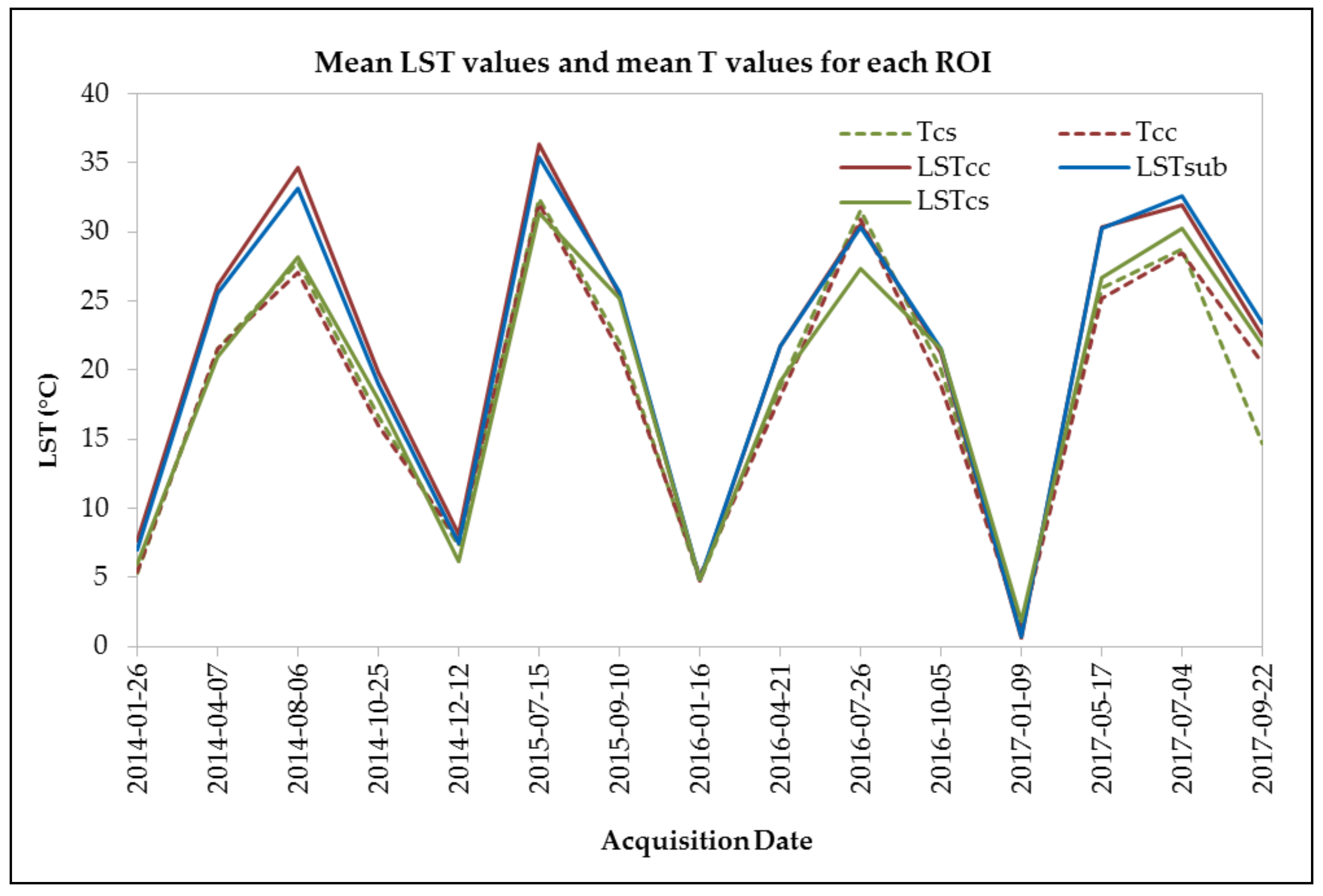
The results showed that with satellite data, the SUHI is clearly visible during hot and mid seasons, while an opposite phenomenon is observed during cold seasons.
In particular, during hot seasons, Modena records a significant SUHI phenomenon, with a difference between City Center LST values and Countryside LST values of up to 6.4 °C.
Observing the entire studied period (from 2014 to 2017), the following assessments can be made:
  • Mean LST values are on average higher from 2014 to 2015 than from 2016 to 2017;
  • The SUHI phenomenon is more evident during hot seasons, especially in the years 2014 and 2015.
These assessments are certainly consistent with the policies implemented by the municipality of Modena in recent years concerning European Green Infrastructures Strategies. Thus, the application of the methodology presented in this paper highlights the mitigation effect on the SUHI (and therefore on the UHI) of the Modena SEAP agreement.
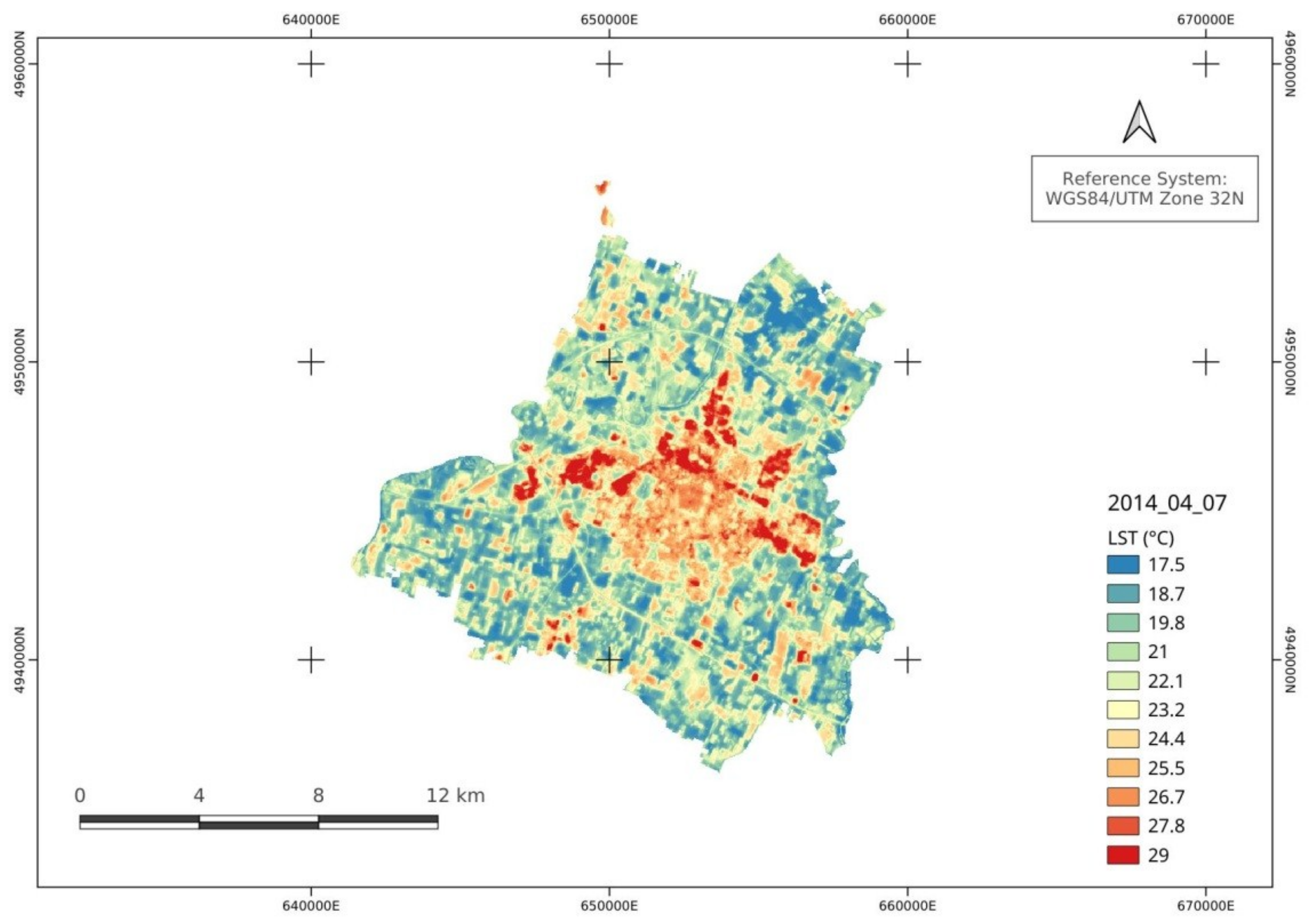
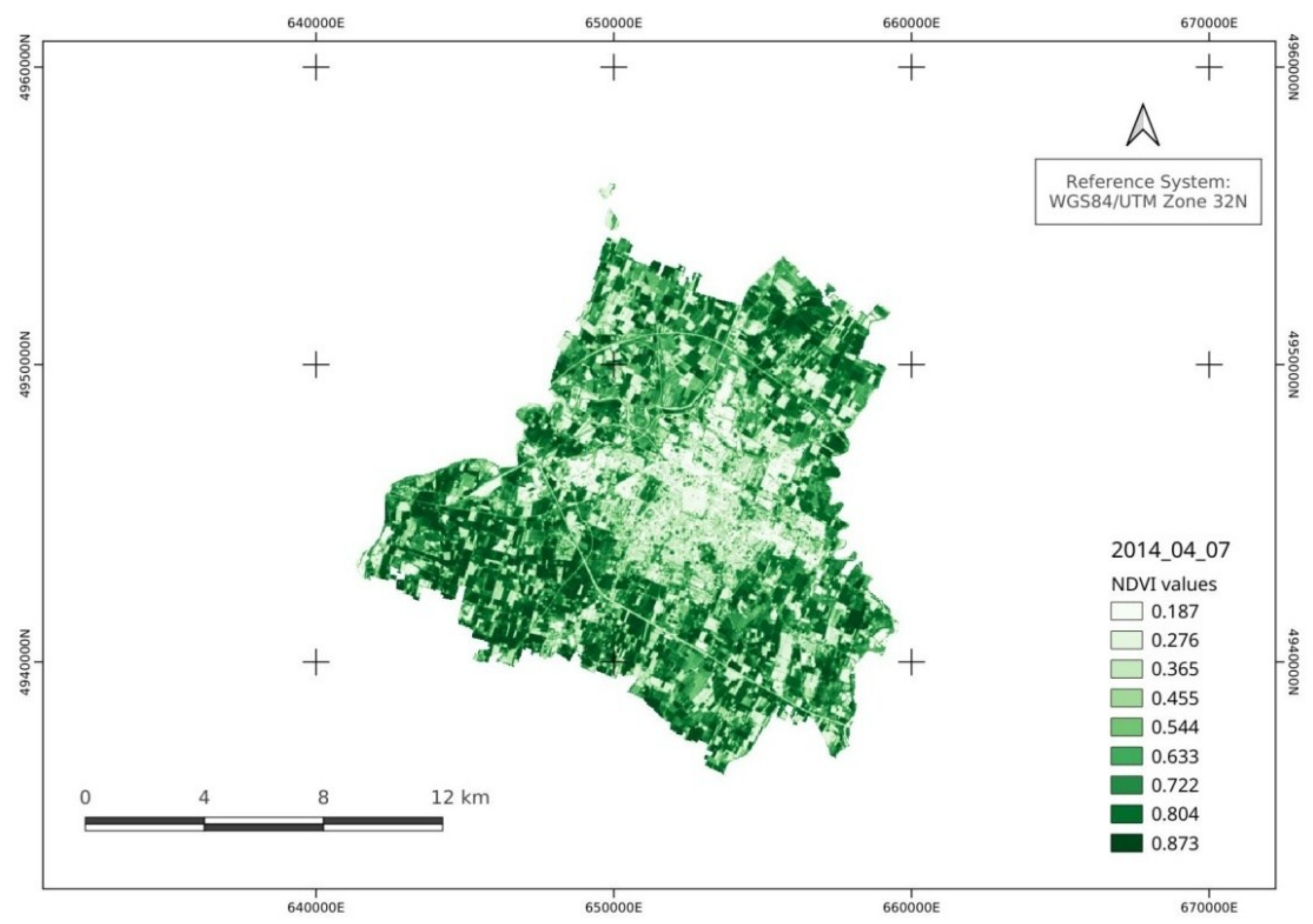
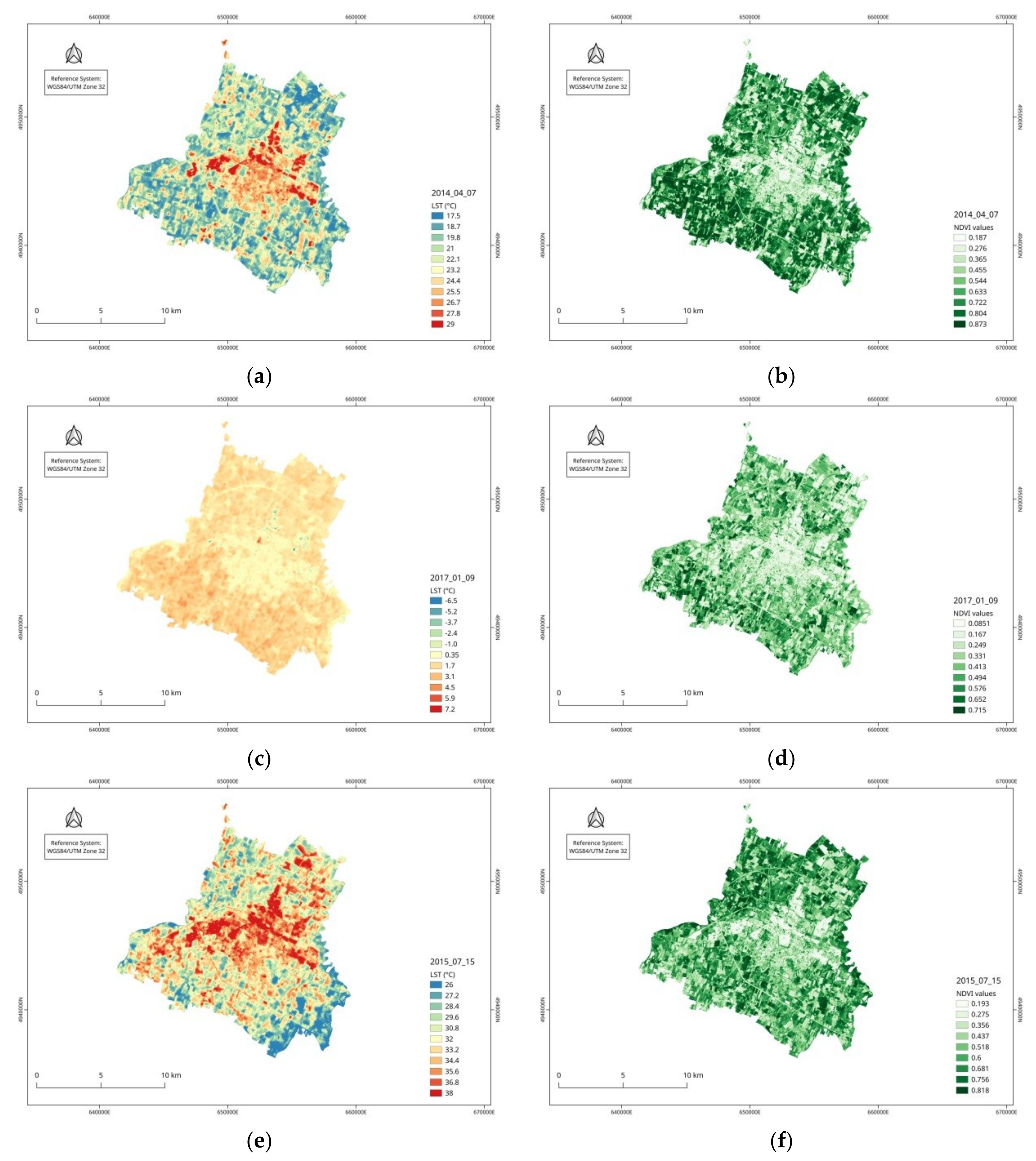
NDVI maps were useful to identify the vegetation cover and to correlate it with LST maps. This study confirmed that, for hot and mid seasons, high values of LST correspond to low values of NDVI (bare soil or artificial covers). For example, for the image of 15 July 2015, the Pearson coefficient (r) shows a correlation between LST values and NDVI values equal to 0.91 for City Center, 0.79 for Suburbs, and 0.77 for Countryside. For the mid season, the correlation between NDVI and LST is still strong. For example, for the image from 7 April 2014, the Pearson coefficient values are between 0.85 and 0.92. Otherwise, during cold seasons, this study revealed a null or opposite trend of the phenomenon and a low correlation between NDVI values and LST values.
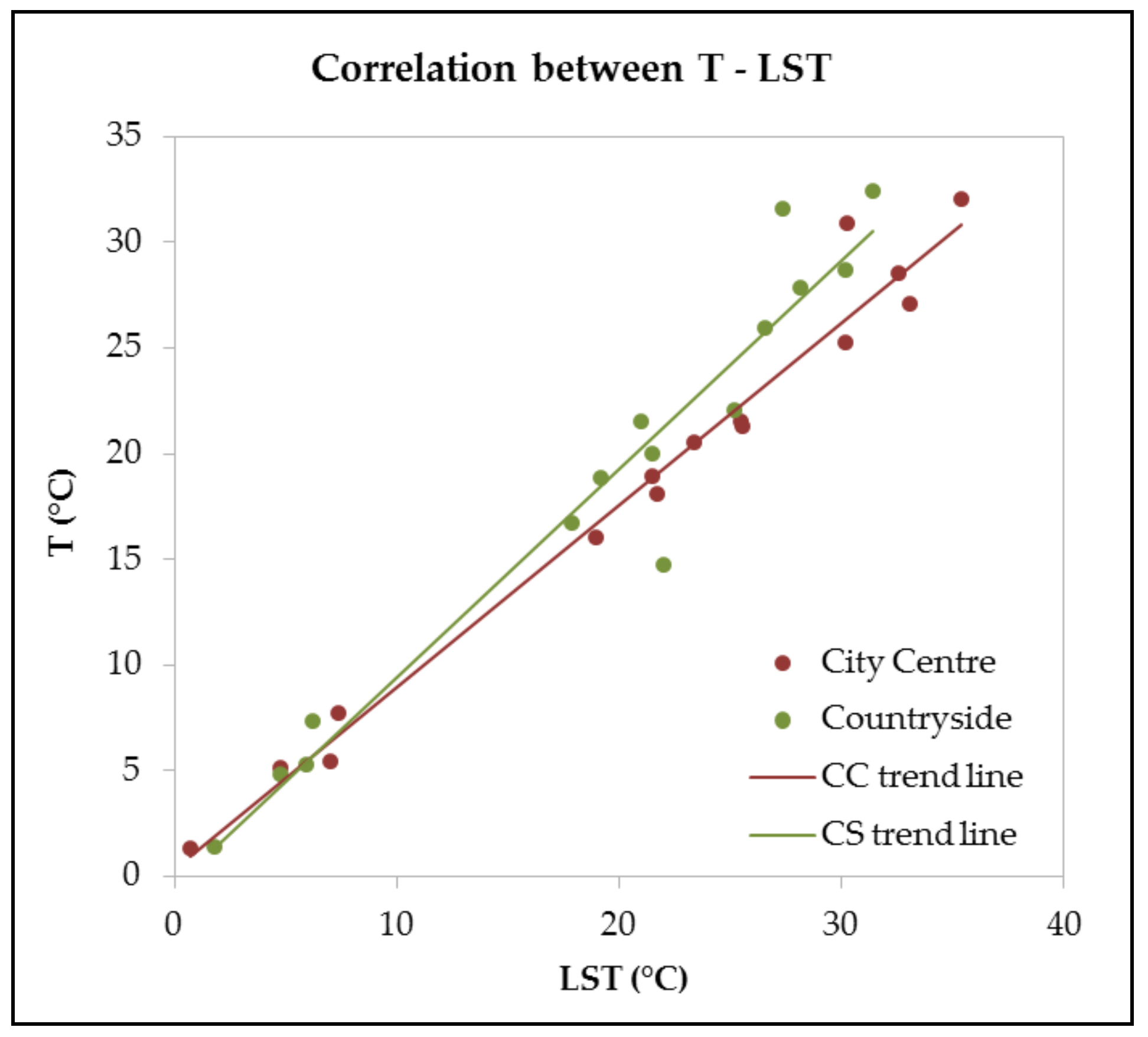
Remote sensing LST values were also compared with air temperature values measured by two weather stations (one for the City Center region and one for the Countryside region). These values showed a high correlation with the Pearson coefficient equal to 0.98 for City Center and to 0.97 for Countryside. Remote sensing data are therefore representative of real surface temperatures and thus they can be used for the identification of the SUHI and the estimation of its intensity.
In conclusion, this study showed that the SUHI is a phenomenon that can also be observed in medium-sized municipalities like Modena and that can be investigated with a free and accessible methodology. The proposed methodology could be easily used not only for the identification of SUHI but also for its intensity estimation thanks to the good correlation between LST values and air temperature values. This study could thus represent a powerful tool for public administration for sustainable planning policies based on UHI mitigation strategies. Using the proposed methodology for several images acquired in different years allows one to monitor the UHI mitigation actions and verify their effect on the territory.
Furthermore, the proposed methodology could be used not only for cities similar to Modena but also for different kind of cities, from large metropolises to small municipalities. For the transferability of the methodology, the choice of ROIs is important: each ROI has to be compared with LCZs definitions in order to set universal benchmarks to compare obtained results.
This study is not concluded. More images will be analyzed, in particular during hot seasons, and, for each image, the Albedo parameter will be calculated to correlate the SUHI to surface reflectance. Moreover, complete meteorological data will be collected in order to better understand the SUHI phenomenon, taking the local climate into consideration. Additionally, data such as the daily precipitation of the three days before the image acquisition time, the average daily wind speed, and the main wind direction will provide a complete climatic and environmental characterization of the acquisition time for each image.

Author Contributions

Conceptualization, F.D.; Data curation, T.B.; Funding acquisition, F.D. and S.T.; Investigation, T.B. and F.D.; Methodology, T.B. and F.D.; Project administration, T.B., F.D., and S.T.; Software, T.B.; Supervision, F.D. and S.T.; Validation, F.D. and S.T.; Visualization, T.B.; Writing—original draft, T.B.; Writing—reviewing and editing, T.B., F.D., and S.T.

Acknowledgments

This work was partially supported by the BRIC INAIL ID 57/2016 Project, CUP B52F17000610005. For the weather data and the climatological analysis of the area, the authors would like to thank the “Osservatorio Geofisico” of Modena (Geophysical Observatory of Modena).

Conflicts of Interest

The authors declare no conflict of interest.

Abbreviations

ARPAEAgenzia Regionale Prevenzione Ambiente ed Energia
DNDigital Number
FVCFractional Vegetation Cover
LCZLocal Climate Zone
LSELand Surface Emissivity
LSTLand Surface Temperature
LWIRLong-Wave Infrared
MODISModerate Resolution Imaging Spectroradiometer
NDVINormalized Difference Vegetation Index
NIRNear Infrared
OLIOperational Land Imager
QGISQuantum Geographic Information System
ROIRegion of Interest
SCPSemi-Automatic Classification Plugin
SEAPPlan of Action for Sustainable Energy
SUHISurface Urban Heat Island
SWIRShort-Wave Infrared
TIRSThermal Infrared Sensor
TOATop of Atmosphere
UHIUrban Heat Island
USGSUnited States Geological Survey
UTCCoordinated Universal Time
VISVisible

References

  1. Brenner, N.; Schmid, C. The ‘Urban Age’ in Question. Int. J. Urban Reg. Res. 2014, 38, 731–755. [Google Scholar] [CrossRef]
  2. McLellan, B.C.; Chapman, A.J.; Aoki, K. Geography, Urbanization and Lock-in-Considerations for Sustainable Transitions to Decentralized Energy Systems. J. Clean. Prod. 2014. [Google Scholar] [CrossRef]
  3. Stewart, I.D. Local Climates of the City. Archit. Des. 2013, 83, 100–105. [Google Scholar] [CrossRef]
  4. Seto, C.K.; Parnell, S.; Elmqvist, T. A Global Outlook on Urbanization. In Urbanization, Biodiversity and Ecosystem Services: Challenges and Opportunities; Springer: Dordrecht, The Netherlands, 2014. [Google Scholar]
  5. Brade, I.; Kovacs, Z. City and Countryside under World-Wide Urbanization. Reg. Res. Russ. 2014, 4, 76–79. [Google Scholar] [CrossRef]
  6. Zhou, Q. A review of sustainable urban drainage systems considering the climate change and urbanization impacts. Water 2014, 6, 976–992. [Google Scholar] [CrossRef]
  7. Prather, H.; Rosenstiel, T.N. Urbanization Impacts on Tree Canopies: The Unexplored Link between Canopy Epiphytes and Pacific Northwest Forest Biogeochemical Cycles. In Proceedings of the AGU Fall Meeting Abstracts, San Francisco, CA, USA, 15–19 December 2014. [Google Scholar]
  8. Li, H.B.; Yu, S.; Li, G.L.; Deng, H.; Xu, B.; Ding, J.; Wong, M.H. Spatial distribution and historical records of mercury sedimentation in urban lakes under urbanization impacts. Sci. Total Environ. 2013, 445, 117–125. [Google Scholar] [CrossRef] [PubMed]
  9. Santamouris, M.; Cartalis, C.; Synnefa, A.; Kolokotsa, D. On the impact of urban heat island and global warming on the power demand and electricity consumption of buildings—A review. Energy Build. 2015, 98, 119–124. [Google Scholar] [CrossRef]
  10. Santamouris, M. On the energy impact of urban heat island and global warming on buildings. Energy Build. 2014, 82, 100–113. [Google Scholar] [CrossRef]
  11. Akbari, Y.W.U.B.H. Comparing the effects of Urban Heat Island Mitigation. J. Mol. Biol. 2015, 342, 131–143. [Google Scholar] [CrossRef]
  12. Babu, S.R.; Aakriti, G. Remote Sensing of Urban Microclimate with Special Reference to Urban Heat Island using Landsat Thermal Data. Geogr. Pol. 2014, 87, 555–568. [Google Scholar] [CrossRef]
  13. Marchesi, S.; Zauli, S.S.; Lauriola, P. Impact of Mitigation Measures on the Urban Heat Island Phenomenon in the City of Modena, Italy. Geogr. Pol. 2014, 87, 531–540. [Google Scholar] [CrossRef]
  14. Kawamoto, Y. Effect of Land-Use Change on the Urban Heat Island in the Fukuoka–Kitakyushu Metropolitan Area, Japan. Sustainability 2017, 9, 1521. [Google Scholar] [CrossRef]
  15. Yuan, F.; Bauer, M.E. Comparison of impervious surface area and normalized difference vegetation index as indicators of surface urban heat island effects in Landsat imagery. Remote Sens. Environ. 2007, 106, 375–386. [Google Scholar] [CrossRef]
  16. Chen, X.L.; Zhao, H.M.; Li, P.X.; Yin, Z.Y. Remote sensing image-based analysis of the relationship between urban heat island and land use/cover changes. Remote Sens. Environ. 2006, 104, 133–146. [Google Scholar] [CrossRef]
  17. Bonafoni, S.; Baldinelli, G.; Verducci, P.; Presciutti, A. Remote Sensing Techniques for Urban Heating Analysis: A Case Study of Sustainable Construction at District Level. Sustainability 2017, 9, 1308. [Google Scholar] [CrossRef]
  18. Rohinton, E. Thermal comfort implications of urbanization in a warm-humid city: The Colombo Metropolitan Region (CMR), Sri Lanka. Build. Environ. 2005, 40, 1591–1601. [Google Scholar]
  19. Van Hove, L.W.A.; Jacobs, C.M.J.; Heusinkveld, B.G.; Elbers, J.A.; Van Driel, B.L.; Holtslag, A.A.M. Temporal and spatial variability of urban heat island and thermal comfort within the Rotterdam agglomeration. Build. Environ. 2015, 83, 91–103. [Google Scholar] [CrossRef]
  20. Sheng, L.; Tang, X.; You, H.; Gu, Q.; Hu, H. Comparison of the urban heat island intensity quantified by using air temperature and Landsat land surface temperature in Hangzhou, China. Ecol. Indic. 2017, 72, 738–746. [Google Scholar] [CrossRef]
  21. Jimenez-Munoz, J.C.; Sobrino, J.A.; Skokovic, D.; Mattar, C.; Cristobal, J. Land Surface Temperature Retrieval Methods from Landsat-8 Thermal Infrared Sensor Data. IEEE Geosci. Remote Sens. Lett. 2014, 11, 1840–1843. [Google Scholar] [CrossRef]
  22. Rozenstein, O.; Qin, Z.; Derimian, Y.; Karnieli, A. Derivation of Land Surface Temperature for Landsat-8 TIRS Using a Split Window Algorithm. Sensors 2014, 14, 5768–5780. [Google Scholar] [CrossRef] [PubMed]
  23. Weng, Q.; Lu, D.; Schubring, J. Estimation of land surface temperature–vegetation abundance relationship for urban heat island studies. Remote Sens. Environ. 2004, 89, 467–483. [Google Scholar] [CrossRef]
  24. Rajeshwari, A.; Mani, N.D. Estimation of land surface temperature of Dindigul district using Landsat 8 data. Int. J. Res. Eng. Technol. 2014, 3, 122–126. [Google Scholar]
  25. Li, H.; Du, Y.; Liu, Q.; Xu, D.; Cao, B.; Jiang, J.; Wang, H. Land Surface Temperature Retrieval from Tiangong-1 Data and its Applications in Urban Heat Island Effect. J. Remote Sens. 2014, 18, 133–143. [Google Scholar] [CrossRef]
  26. Benas, N.; Chrysoulakis, N.; Cartalis, C. Trends of urban surface temperature and heat island characteristics in the Mediterranean. Theor. Appl. Climatol. 2016, 1–10. [Google Scholar] [CrossRef]
  27. Schwarz, N.; Uwe, S.; Ulrich, F.; Großmann, K. Relationship of Land Surface and Air Temperatures and Its Implications for Quantifying Urban Heat Island Indicators—An Application for the City of Leipzig (Germany). Ecol. Indic. 2012, 18, 693–704. [Google Scholar] [CrossRef]
  28. Wang, H.; Yuanzhi, Z.; Jin, T.; Yu, L. Surface Urban Heat Island Analysis of Shanghai (China) Based on the Change of Land Use and Land Cover. Sustainability 2017, 9, 1538. [Google Scholar] [CrossRef]
  29. Despini, F.; Ferrari, C.; Bigi, A.; Libbra, A.; Teggi, S.; Muscio, A.; Ghermandi, G. Correlation between Remote Sensing Data and Ground Based Measurements for Solar Reflectance Retrieving. Energy Build. 2016, 114, 227–233. [Google Scholar] [CrossRef]
  30. García-Cueto, O.R.; Jauregui-Ostos, E.; Toudert, D.; Tejeda-Martinez, A. Detection of the urban heat island in Mexicali, BC, México and its relationship with land use. Atmósfera 2007, 20, 111–131. [Google Scholar]
  31. Hartz, D.A.; Prashad, L.; Hedquist, B.C.; Golden, J.; Brazel, A.J. Linking satellite images and hand-held infrared thermography to observed neighborhood climate conditions. Remote Sens. Environ. 2006, 104, 190–200. [Google Scholar] [CrossRef]
  32. Lindberg, F. Modelling the urban climate using a local governmental geo-database. Meteorol. Appl. 2007, 14, 263–273. [Google Scholar] [CrossRef]
  33. Voogt, J.A.; Oke, T.R. Thermal remote sensing of urban climates. Remote Sens. Environ. 2003, 86, 370–384. [Google Scholar] [CrossRef]
  34. Bornstein, R.D. Observations of the urban heat island effect in New York City. J. Appl. Meteorol. 1968, 7, 575–582. [Google Scholar] [CrossRef]
  35. Feng, H.; Zhao, X.; Chen, F.; Wu, L. Using land use change trajectories to quantify the effects of urbanization on urban heat island. Adv. Space Res. 2014, 53, 463–473. [Google Scholar] [CrossRef]
  36. Takebayashi, H.; Moriyama, M. Surface heat budget on green roof and high reflection roof for mitigation of urban heat island. Build. Environ. 2007, 42, 2971–2979. [Google Scholar] [CrossRef]
  37. Zinzi, M.; Agnoli, S. Cool and green roofs. An energy and comfort comparison between passive cooling and mitigation urban heat island techniques for residential buildings in the Mediterranean region. Energy Build. 2012, 55, 66–76. [Google Scholar] [CrossRef]
  38. Ferrari, C.; Libbra, A.; Muscio, A.; Siligardi, C. Influence of the irradiance spectrum on solar reflectance measurements. Adv. Build. Energy Res. 2013, 7, 244–253. [Google Scholar] [CrossRef]
  39. Kazak, K.J. The Use of a Decision Support System for Sustainable Urbanization and Thermal Comfort in Adaptation to Climate Change Actions—The Case of the Wrocław Larger Urban Zone (Poland). Sustainability 2018, 10, 1083. [Google Scholar] [CrossRef]
  40. Santamouris, M. Analyzing the heat island magnitude and characteristics in one hundred Asian and Australian cities and regions. Sci. Total Environ. 2015, 512–513, 582–598. [Google Scholar] [CrossRef] [PubMed]
  41. Lee, S.; Hyunbin, M.; Yeri, C.; Yoon, D.K. Analyzing Thermal Characteristics of Urban Streets Using a Thermal Imaging Camera: A Case Study on Commercial Streets in Seoul, Korea. Sustainability 2018, 10, 519. [Google Scholar] [CrossRef]
  42. Salvati, A.; Coch Roura, H.; Cecere, C. Assessing the urban heat island and its energy impact on residential buildings in Mediterranean climate: Barcelona case study. Energy Build. 2017, 146, 38–54. [Google Scholar] [CrossRef]
  43. Giannopoulou, K.; Livada, I.; Santamouris, M.; Saliari, M.; Assimakopoulos, M.; Caouris, Y.G. On the characteristics of the summer urban heat island in Athens, Greece. Sustain. Cities Soc. 2011, 1, 16–28. [Google Scholar] [CrossRef]
  44. Santamouris, M. Challenges and priorities for a sustainable built environment in Southern Europe-the impact of energy efficiency measures and renewable energies on employment. In Energy Performance of Buildings: Energy Efficiency and Built Environment in Temperate Climates; Springer: Cham, Switzerland, 2015; pp. 63–77. [Google Scholar]
  45. Giannaros, T.M.; Melas, D. Study of the urban heat island in a coastal Mediterranean City: The case study of Thessaloniki, Greece. Atmos. Res. 2012, 118, 103–120. [Google Scholar] [CrossRef]
  46. Saaroni, H.; Ben-Dor, E.; Bitan, A.; Potchter, O. Spatial distribution and microscale characteristics of the urban heat island in Tel-Aviv, Israel. Landsc. Urban Plan. 2000, 48, 1–18. [Google Scholar] [CrossRef]
  47. Colacino, M.; Lavagnini, A. Evidence of the urban heat island in Rome by climatological analyses. Arch. Meteorol. Geophys. Bioclimatol. Ser. B 1982, 31, 87–97. [Google Scholar] [CrossRef]
  48. Bacci, P.; Maugeri, M. The urban heat island of Milan. Nuovo Cim. C 1992, 15, 417–424. [Google Scholar] [CrossRef]
  49. Anniballe, R.; Bonafoni, S.; Pichierri, M. Spatial and temporal trends of the surface and air heat island over Milan using MODIS data. Remote Sens. Environ. 2014, 150, 163–171. [Google Scholar] [CrossRef]
  50. Guattari, C.; Evangelisti, L.; Balaras, C.A. On the assessment of urban heat island phenomenon and its effects on building energy performance: A case study of Rome (Italy). Energy Build. 2018, 158, 605–615. [Google Scholar] [CrossRef]
  51. Sajani, S.Z.; Marchesi, S.; Lauriola, P.; Tomozeiu, R.; Botarelli, L.; Bonafè, G.; Guaragno, G.; Fiumi, F.; Zanelli, M.; Gherardi, L.; et al. UHI in the metropolitan cluster of bologna-modena: Mitigation and adaptation strategies. In Counteracting Urban Heat Island Effects in a Global Climate Change Scenario; Springer: Cham, Switzerland, 2016; pp. 131–200. [Google Scholar]
  52. Busato, F.; Lazzarin, R.M.; Noro, M. Three years of study of the Urban Heat Island in Padua: Experimental results. Sustain. Cities Soc. 2014, 10, 251–258. [Google Scholar] [CrossRef]
  53. Peron, F.; De Maria, M.M.; Spinazzè, F.; Mazzali, U. An analysis of the urban heat island of Venice mainland. Sustain. Cities Soc. 2015, 19, 300–309. [Google Scholar] [CrossRef]
  54. Morabito, M.; Crisci, A.; Gioli, B.; Gualtieri, G.; Toscano, P.; Di Stefano, V.; Orlandini, S.; Gensini, G.F. Urban-hazard risk analysis: Mapping of heat-related risks in the elderly in major Italian cities. PLoS ONE 2015, 10, e0127277. [Google Scholar] [CrossRef] [PubMed]
  55. Bonafè, G. Microclima Urbano: Impatto Dell’urbanizzazione Sulle Condizioni Climatiche Locali e Fattori di Mitigazione; Area Meteorologica Ambientale, Servizio IdroMeteorologico, ARPA: Emilia Romagna, Italy, 2006. [Google Scholar]
  56. Mahdavi, A.; Kiesel, K.; Vuckovic, M. Methodologies for UHI Analysis. In Counteracting Urban Heat Island Effects in a Global Climate Change Scenario; Springer: Cham, Switzerland, 2016; pp. 71–91. [Google Scholar]
  57. Caserini, S.; Giani, P.; Cacciamani, C.; Ozgen, S.; Lonati, G. Influence of climate change on the frequency of daytime temperature inversions and stagnation events in the Po Valley: Historical trend and future projections. Atmos. Res. 2017, 184, 15–23. [Google Scholar] [CrossRef]
  58. Putaud, J.P.; Cavalli, F.; Dos Santos, M.; Dell’Acqua, A. Long-Term Trends in Aerosol Optical Characteristics in the Po Valley, Italy. Atmos. Chem. Phys. 2014, 14, 9129–9136. [Google Scholar] [CrossRef] [Green Version]
  59. Qiu, G.Y.; Li, H.Y.; Zhang, Q.T.; Chen, W.; Liang, W.J.; Li, X.Z. Effects of Evapotranspiration on Mitigation of Urban Temperature by Vegetation and Urban Agriculture. J. Integr. Agric. 2013, 12, 1307–1315. [Google Scholar] [CrossRef]
  60. Zhang, X.; Hu, L.; Bian, X.; Zhao, B.; Chai, F.; Sun, X. The most economical irrigation amount and evapotranspiration of the turfgrasses in Beijing City, China. Agric. Water Manag. 2007, 89, 98–104. [Google Scholar] [CrossRef]
  61. Grimmond, C.S.B.; Oke, T.R. Evapotranspiration rates in urban areas. In Impact of Urban. Growth on Surface Water and Groundwater Quality; IAHS Publication: Wallingford, UK, 1999; Volume 259, pp. 235–244. [Google Scholar]
  62. European Commission. Supporting the Implementation of Green Infrastructure—Final Report. 2016. Available online: http://ec.europa.eu/environment/nature/ecosystems/docs/green_infrastructures/GI%20Final%20Report.pdf (accessed on 8 May 2018).
  63. The Covenant of Mayors. Piano di Azione per L’energia Sostenibile. 2011. Available online: http://www.pattosindacimodena.it/index.php?option=com_docman&task=doc_view&gid=31&Itemid=77 (accessed on 8 May 2018).
  64. Huang, M.; Peng, C.; Xin, H. Study of the Cooling Effects of Urban Green Space in Harbin in Terms of Reducing the Heat Island Effect. Sustainability 2018, 10, 1101. [Google Scholar] [CrossRef]
  65. Wang, Y.; Qingming, Z.; Wanlu, O. Impact of Urban Climate Landscape Patterns on Land Surface Temperature in Wuhan, China. Sustainability 2017, 9, 1700. [Google Scholar] [CrossRef]
  66. QGIS Development Team, QGIS Geographic Information System. Open Source Geospatial Foundation. 2009. Available online: http://qgis.osgeo.org (accessed on 26 April 2016).
  67. Congedo, L. Semi-Automatic Classification Plugin documentation. Release 2016, 225–235. [Google Scholar] [CrossRef]
  68. Ivajnšič, D.; Kaligarič, M.; Žiberna, I. Geographically Weighted Regression of the Urban Heat Island of a Small City. Appl. Geogr. 2014, 53, 341–353. [Google Scholar] [CrossRef]
  69. Kim, J.P.; Guldmann, J.M. Land-use Planning and the Urban Heat Island. Environ. Plan. B Plan. Des. 2014, 41, 1077–1099. [Google Scholar] [CrossRef]
  70. Masumoto, K. Urban Heat Islands. Environ. Indic. 2015, 67–75. [Google Scholar] [CrossRef]
  71. Statistiche Demografiche ISTAT. Available online: www.demoistat.it (accessed on 31 March 2017).
  72. Costanzini, S.; Teggi, S.; Bigi, A.; Ghermandi, G.; Filippini, T.; Malagoli, C.; Vinceti, M. Atmospheric Dispersion Modelling and Spatial Analysis to Evaluate Population Exposure to Pesticides from Farming Processes. Atmosphere 2018, 9, 38. [Google Scholar] [CrossRef]
  73. Lombroso, L.; Quattrocchi, S. L’Osservatorio di Modena: Inquadramento geografico. La temperatura dell’aria. Le precipitazioni. In L’osservatorio di Modena: 180 Anni di Misure Meteoclimatiche, 1st ed.; Società Meteorologica Subalpina: Moncalieri, Italy, 2008; ISBN 978-88-9-030232-9. [Google Scholar]
  74. Osservatorio Geofisico. Available online: http://meteo.unimore.it/meteo/ (accessed on 8 May 2018).
  75. Bigi, A.; Ghermandi, G. Long-term trend and variability of atmospheric PM 10 concentration in the Po Valley. Atmos. Chem. Phys. 2014, 14, 4895–4907. [Google Scholar] [CrossRef] [Green Version]
  76. Roy, D.P.; Wulder, M.A.; Loveland, T.R.; Woodcock, C.E.; Allen, R.G.; Anderson, M.C.; Scambos, T.A. Landsat-8: Science and product vision for terrestrial global change research. Remote Sens. Environ. 2014, 145, 154–172. [Google Scholar] [CrossRef]
  77. Knight, E.J.; Kvaran, G. Landsat-8 operational land imager design, characterization and performance. Remote Sens. 2014, 6, 10286–10305. [Google Scholar] [CrossRef]
  78. Chander, G.; Markham, B. Revised Landsat-5 TM radiometric calibration procedures and postcalibration dynamic ranges. IEEE Trans. Geosci. Remote Sens. 2003, 41, 2674–2677. [Google Scholar] [CrossRef]
  79. Markham, B.; Barsi, J.; Kvaran, G.; Ong, L.; Kaita, E.; Biggar, S.; Helder, D. Landsat-8 operational land imager radiometric calibration and stability. Remote Sens. 2014, 6, 12275–12308. [Google Scholar] [CrossRef]
  80. Smith, R.B.; Bonneau, L.; Lee, X.; Woo, L.; Fein, F. Yale University, Yale Guide to Landsat 8 Image Processing; The Yale Center for Earth Observation: Yale, CT, USA, 2013; pp. 1–6. [Google Scholar]
  81. Coll, C.; Galve, J.M.; Sánchez, J.M.; Caselles, V. Validation of Landsat-7/ETM+ Thermal-Band Calibration and Atmospheric Correction with Ground-Based Measurements. IEEE Trans. Geosci. Remote Sens. 2010, 48, 547–555. [Google Scholar] [CrossRef]
  82. Stewart, I.D.; Oke, T.R. A New Classification System for Urban Climate Sites. 2009. Available online: https://search.proquest.com/openview/ed3c2a1f4ad2a582f178eb25f3141e90/1?pq-origsite=gscholar&cbl=31345 (accessed on 22 May 2018).
  83. Stewart, I.D.; Oke, T.R. Local climate zones for urban temperature studies. Bull. Am. Meteorol. Soc. 2012, 93, 1879–1900. [Google Scholar] [CrossRef]
  84. Kolokotsa, D.; Psomas, A.; Karapidakis, E. Urban heat island in southern Europe: The case study of Hania, Crete. Sol. Energy 2009, 83, 1871–1883. [Google Scholar] [CrossRef]
  85. Vardoulakis, E.; Karamanis, D.; Fotiadi, A.; Mihalakakou, G. The urban heat island effect in a small Mediterranean city of high summer temperatures and cooling energy demands. Sol. Energy 2013, 94, 128–144. [Google Scholar] [CrossRef]
  86. Fabrizi, R.; Bonafoni, S.; Biondi, R. Satellite and ground-based sensors for the Urban Heat Island analysis in the city of Rome. Remote Sens. 2010, 2, 1400–1415. [Google Scholar] [CrossRef]
  87. Jiang, Z.; Huete, A.R.; Chen, J.; Chen, Y.; Li, J.; Yan, G.; Zhang, X. Analysis of NDVI and scaled difference vegetation index retrievals of vegetation fraction. Remote Sens. Environ. 2006, 101, 366–378. [Google Scholar] [CrossRef]
  88. Ke, Y.; Im, J.; Lee, J.; Gong, H.; Ryu, Y. Characteristics of Landsat 8 OLI-derived NDVI by comparison with multiple satellite sensors and in-situ observations. Remote Sens. Environ. 2015, 164, 298–313. [Google Scholar] [CrossRef]
Figure 1. Ortho image of the city from an aerial photograph of Modena provided by the cartographic archive of the Emilia Romagna region (AGEA 2011). the municipality borders are shown in red (Source: Geodatabase Emilia Romagna region—http://geoportale.regione.emilia-romagna.it, image elaborated by the authors).
Sustainability 10 01678 g001
Figure 2. Digital Terrain Model (DTM) of Italy with the location of the city of Modena. (Source: The Ministry of the Environment and Protection of Land and Sea of Italy—www.pcn.minambiente.it/mattm/, image elaborated by the authors).
Sustainability 10 01678 g002
Figure 3. Conceptual diagram of the proposed methodology.
Sustainability 10 01678 g003
Figure 4. Land Surface Temperature (LST) map of Modena, 7 April 2014. (Source: Quantum Geographic Information System (QGIS) elaboration of LST map provided by the authors).
Sustainability 10 01678 g004
Figure 5. LST map of Modena, 9 January 2017. (Source: QGIS elaboration of LST map provided by the authors).
Sustainability 10 01678 g005
Figure 6. Region of Interest (ROI) map of Modena. ROIs shapefile source: municipality of Modena. (Source: Geodatabase Emilia Romagna region—http://geoportale.regione.emilia-romagna.it, image elaborated by the authors).
Sustainability 10 01678 g006
Figure 7. Mean LST values for each ROI from 2014 to 2017 compared with air temperature values for City Center (TCC) and Countryside (TCS). (Source: Data elaboration provided by the authors).
Sustainability 10 01678 g007
Figure 8. Scatterplot showing the correlation between air temperature (T) and LST considering the whole dataset. (Source: Data elaboration provided by the authors).
Sustainability 10 01678 g008
Figure 9. Normalized Different Vegetation Index (NDVI) map of Modena, 7 April 2014. (Source: QGIS elaboration of NDVI map provided by the authors).
Sustainability 10 01678 g009
Figure 10. (a) LST map of Modena, 7 April 2014. (b) NDVI map of Modena, 7 April 2014. (c) LST map of Modena, 9 January 2017. (d) NDVI map of Modena, 9 January 2017. (e) LST map of Modena, 15 July 2015. (f) NDVI map of Modena, 15 July 2015. (Source: QGIS elaboration of LST and NDVI maps provided by the authors).
Sustainability 10 01678 g010
Table 1. Seasonal mean temperature, seasonal mean of the maximum daily temperatures, seasonal mean of the minimum daily temperatures, and seasonal mean of precipitation of Modena between 1971 and 2000 (historical series) and between 2001 and 2017 (Source: Osservatorio Geofisico di Modena).
Historical series from 1971 to 2000
SeasonTM (°C)TMAXM (°C)TMINM (°C)PrecM (mm)
Spring17.521.713.353.5
Summer23.127.318.849.5
Autumn8.811.26.362.2
Winter5.88.72.940.6
Time series from 2001 to 2017
SeasonTM (°C)TMAXM (°C)TMINM (°C)PrecM (mm)
Spring19.523.715.360.5
Summer24.528.720.345.9
Autumn10.412.98.067.5
Winter7.210.14.253.8
TM: seasonal mean temperature; TMAXM: seasonal mean of the maximum daily temperatures; TMINM: seasonal mean of the minimum daily temperatures; PrecM: seasonal mean of precipitation.
Table 2. Operational Land Imager (OLI) and Thermal Infrared Sensor (TIRS) (Landsat-8) spectral bands.
Spectral BandWavelength (µm)Spatial Resolution (m)
Band 1—Coastal/Aerosol0.435–0.45130
Band 2—Blue0.452–0.51230
Band 3—Green0.533–0.59030
Band 4—Red0.636–0.67330
Band 5—NIR0.851–0.87930
Band 6—SWIR1.566–1.65130
Band 7—SWIR2.107–2.29430
Band 8—Panchromatic0.503–0.67615
Band 9—Cirrus1.363–1.38430
Band 10—LWIR10.60–11.19100 (resampled to 30)
Band 11—LWIR11.50–12.51100 (resampled to 30)
Table 3. Image dataset used in this study.
Acquisition DateDay of the WeekSeasonAcquisition Time—Coordinated Universal Time (UTC)
26 January 2014SundayCold10.00
7 April 2014MondayMid10.00
6 August 2014WednesdayHot10.00
25 October 2014SaturdayMid10.00
12 December 2014FridayCold10.00
15 January 2015WednesdayHot10.00
10 September 2015ThursdayMid10.00
16 January 2016SaturdayCold10.00
21 April 2016ThursdayMid10.00
26 July 2016TuesdayHot10.00
5 October 2016WednesdayMid10.00
9 January 2017MondayCold10.00
17 May 2017WednesdayHot10.00
4 July 2017TuesdayHot10.00
22 September 2017FridayMid10.00
Table 4. Average LST value of each ROI for the processed images.
DateSeasonLST Mean (°C)
City CenterSuburbsCountrysideΔLST (LSTCC − LSTCS)
26 January 2014Cold7.67.05.91.7
7 April 2014Mid26.125.521.05.1
6 August 2014Hot34.633.128.26.4
25 October 2014Mid19.919.017.92.0
12 December 2014Cold8.17.46.21.9
15 January 2015Hot36.335.431.45.2
10 September 2015Mid25.425.625.20.2
16 January 2016Cold4.84.84.80.0
21 April 2016Mid21.721.719.22.5
26 July 2016Hot30.530.327.43.1
5 October 2016Mid21.221.521.5−0.3
9 January 2017Cold0.70.71.8−1.1
17 May 2017Mid30.330.226.63.7
4 July 2017Hot32.032.630.21.8
22 September 2017Mid22.423.422.00.4
Table 5. Minimum ΔLST and maximum ΔLST divided by seasons.
SeasonΔLSTmin–ΔLSTmax (°C)
Hot(6.4)–(1.8)
Mid(−0.3)–(5.1)
Cold(−1.1)–(1.9)
Table 6. Summer Urban Heat Island (UHI) intensity for major Italian cities.
CityMethodology for UHI Intensity EstimationSummer UHI Intensity (°C)References
MilanRemote sensing data
(Moderate Resolution Imaging Spectroradiometer—MODIS sensor)
Maximum of 8–10 °CAnniballe et al., 2014 [49]
RomeTemperature data collected by meteorological stations/remote sensing data2.5–7.5 °CGuattari et al., 2018 [50]
Fabrizi et al., 2010 [86]
Bologna-ModenaTemperature data collected by meteorological stations4–8 °CZauli Sajani et al., 2016 [51]
PaduaTemperature data collected by meteorological stations2–6 °CBusato et al., 2014 [52]
VeniceTemperature data collected by meteorological stations4–7 °CPeron et al., 2015 [53]
Table 7. Pearson coefficient of LST vs. T for each ROI.
ROIPearson Coefficient r
City Center0.98
Countryside0.97
Table 8. Pearson correlation coefficient r between LST and NDVI for each ROI of Modena within different images (“Modena 7 April 2014”, “Modena 15 July 2015” and “Modena 9 January 2017”).
DateROIPearson Coefficient r
7 April 2014City Center0.92
Suburbs0.85
Countryside0.88
15 July 2015City Center0.91
Suburbs0.79
Countryside0.77
9 January 2017City Center0.14
Suburbs0.20
Countryside0.06

