Article

Developing a Model to Assess the Potential Impact of TUM Hydropower Turbines on Small River Ecology

1
Key Laboratory of Environmental Remediation, Institute of Geographic Sciences and Natural Resources Research, China Academy of Sciences, Beijing 100101, China
2
Department of Civil, Geo and Environmental Engineering, Technical University of Munich (TUM), Arcisstrasse 21, 80333 Munich, Germany
3
State Key Laboratory of Hydrology-Water Resources and Hydraulic Engineering, Hohai University, Nanjing 210098, China
4
College of Water Resources and Architectural Engineering, Northwest A&F University, Yangling 712100, China
5
Key Laboratory of Agricultural Soil and Water Engineering in Arid Regions of Ministry of Education, Northwest A&F University, Yangling 712100, China
6
Powerchina Guiyang Engineering Corporation Limited, Guizhou 550081, China
*
Author to whom correspondence should be addressed.
Sustainability 2018, 10(5), 1662; https://doi.org/10.3390/su10051662
Submission received: 31 March 2018 / Revised: 4 May 2018 / Accepted: 7 May 2018 / Published: 21 May 2018
(This article belongs to the Section Environmental Sustainability and Applications)

Abstract

:
Small hydropower is a renewable energy technology that is used for electricity generation worldwide, but still has potential for further development. However, during the installation of small hydropower, the ecological impacts of the power plants need to be thoroughly investigated. In addressing the challenges of energy production and minimizing the environmental impacts of small hydropower installation and operation, this study has applied an ecohydraulic model to investigate river hydrodynamics, hydromorphology, habitat, and the population impacts of small hydropower, and presented the Mum River as a case study. Two scenarios were implemented in this research to simulate the hydrodynamic, sedimentation, habitat, and population status in order to assess the potential effects caused by the TUM plant. At the Mum River, two scenarios were proposed: the TUM plant was not considered in scenario S1, but was considered in scenario S2. The model results for scenario S2 indicated that the habitat was suitable for fish species living in the Mum River, with fish population numbers between 4.6 × 10³ and 6.6 × 10³. The S2 results indicated that the impacts of the TUM plant were negligible when compared with S1. Although the impact of the TUM plant on the Mum River is relatively large when the discharge is high (19 m3/s), calculations based on stable flow shows that the TUM plant could function well on the river ecosystem when the discharge is low or at normal rates. Therefore, this study shows that the TUM plant would be a good option to meet the needs of energy generation whilst having a minimal impact on river habitats and changes in fish species population in similar small rivers and streams.

Graphical Abstract

1. Introduction

Currently, hydropower sources play a significant role in meeting the global energy demand. Compared with wind and solar energy, hydropower is the top-ranking renewable source used to produce electricity [1,2,3,4]. Hydropower electricity represents 13.2% of the total electricity generated in the European Union [5] and 17% of the total electricity generated in China [6]. In many other countries, the proportion of hydropower energy output exceeds 20% [7,8]. However, large-scale hydropower has often been considered ecologically unfriendly [9]. Similar to large-scale hydropower plants, small-scale power plants are also well-developed, reliable, flexible in operation, easy to maintain, and financially competitive [10,11,12,13]. With growing energy demand, small hydropower has experienced a rapid development in Europe and the United States, and has the potential for further expansion, especially in emerging economies [13,14]. For example, small hydropower contributed over 40 GW of world capacity in 2000; in 2011, its potential was more than 1000 GW, and it is expected to increase a further 1400 GW in 2020 [15,16]. China alone developed more than 59 GW in 2011, and accounted for 55.3% of the hydropower sources [16]. There are numerous studies and evaluations of large-scale hydropower plants’ impact river and fish ecosystems [17]. However, how small hydropower plants impact the fish ecosystem also needs to be investigated in detail. This paper focuses on the development of an ecohydraulic model to assess the ecological impact of one specific type of small-scale shaft power plant on river ecosystems.
Small hydropower plants are usually installed in small rivers and streams, and their installation impact on the river and fish ecosystem has started to draw attention from researchers [18]. The ecosystems in small streams are relatively fragile, and are difficult to recover once destroyed [19,20]. Kibler and Tullos [21] also indicate that the biophysical impacts of small hydropower may be serious. Thus, it is essential to evaluate the ecological effects of small hydropower plants, which would help set up comprehensive standards for ecological impact assessment. Among the various evaluation methods, habitat models are particularly useful for assessing the ecological impacts of both large-scale and small-scale hydropower projects [22,23,24,25]. The first habitat model was developed in the 1970s by the United States Fish and Wildlife Service (USFWS) [26,27,28]. Since then, habitat models have shifted from narrow studies that concentrate on one single method to a more holistic approach. Other habitat models have also been developed, and include the PHABSIM, CASiMiR, MesoHABSIM, River2D, EVHA, WW-Eco-Tools, and HABSCORE models [29,30,31,32,33,34].
Besides the habitat model, population models have also been recommended as an effective and accurate approach for assessing fish population variations, the effects of river managements, and dam constructions. One example is the ecohydraulic model system, which can be used to describe fish abundance fluctuations and fish density distributions [35,36]. Other population models have been developed, and include the individual-based model (IBM) [37,38,39]; the InSTREAM model [40] and the Salmon model [41,42]. Based on previous habitat and population model concepts, a new ecohydraulic model system was proposed that was suitable for assessing the ecological impacts of the TUM plants on the Mum River. TUM plants are a typical new concept small power plant, and the Mum River was selected as the case study for this paper. In this paper, the ecohydraulic model system was applied to assess the effects of TUM plant construction on river hydrodynamics, sedimentations, ecologies, and fish abundances. The ecohydraulic model system included a hydrodynamic model, a sediment transport model, a habitat model, and a population model [43,44,45,46,47]. It was important to assess the changes in habitat quality and any fish population variations caused by the construction of the TUM plant, as the quantitative analysis of these effects would allow the development of an approach that could define the ecological impacts of a TUM plant and minimize the negative influences of its construction.
The aim of this paper is to: (1) propose an ecohydraulic model system to simulate the fish habitat quality and fish population status on the Mum River; (2) use an ecohydraulic model system to evaluate the effects of the TUM plant construction on fish habitat quality and abundance on the Mum River; and (3) analyze the sensitivity of the TUM plant effects on hydrodynamics, habitat quality, and fish abundance on the Mum River.

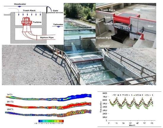
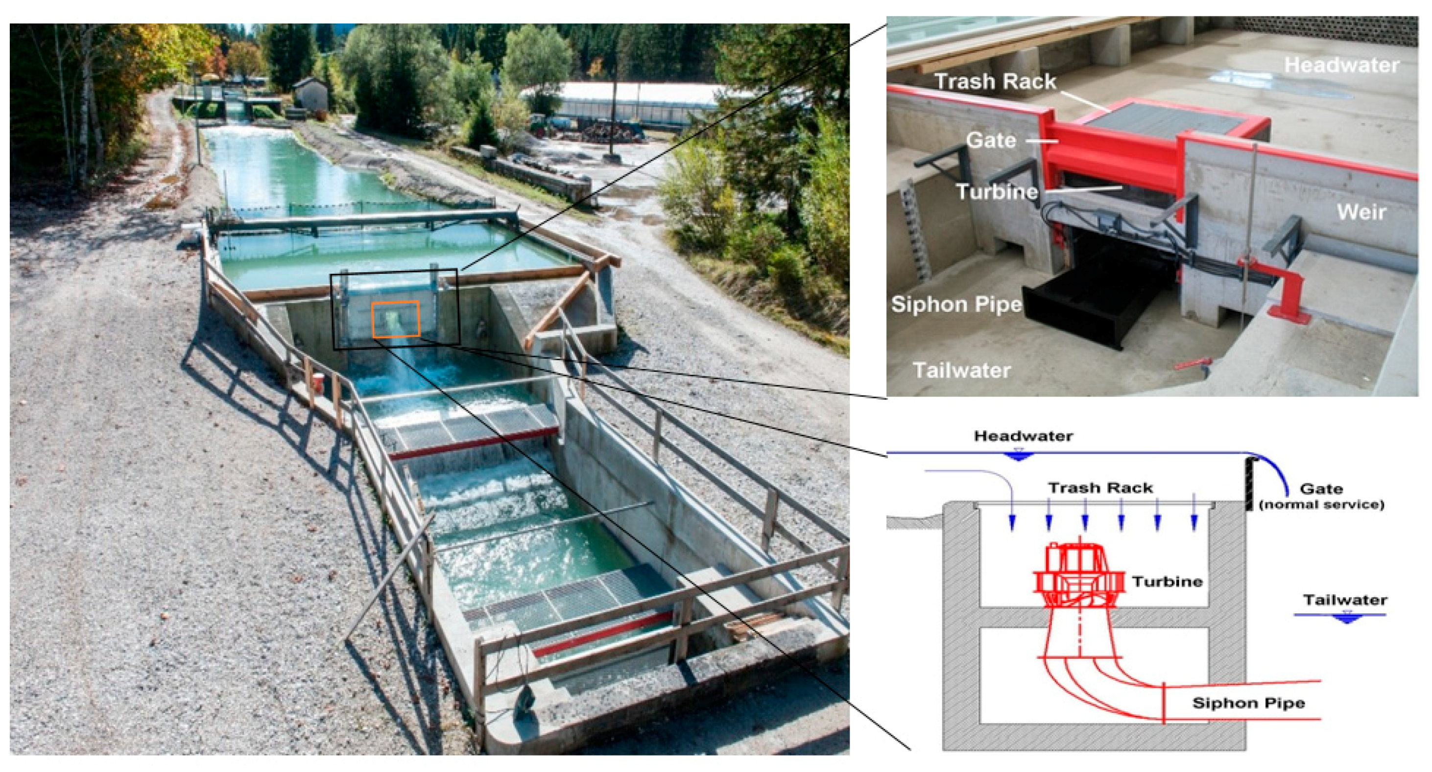
2. Technical Aspects of the Shaft Power Plant and Study Area

The TUM plant was designed by the Technical University of Munich, and consists of a concrete box, a sliding gate, and a dive turbine with a propeller (Figure 1) [48,49]. This plant fulfills the framework of the environmental constraints, the German Water Management Act of 2010, and the European Union (EU) Water Framework Directive [50]. The maximum output of a TUM plant is 5 MW. Figure 1 shows the concrete box ( 2   m   ×   2   m   ×   2.5   m ), sitting just upstream of an existing weir. It also shows the sliding gate which, during regular operations, is partly overflowed with water to prevent air from entraining vortices and enable fish to migrate downstream. The TUM plant is equipped with a dive turbine with a propeller, runner, and generator sitting below the water surface. The measurements of the TUM plant efficiency ranges from 86% to 88% [51]. Figure 1 shows how the flow is directed from the horizontal into the vertical shaft portion, through the turbine and the suction pipe, and into the downstream river section.
This TUM plant encompasses several specific concepts: a vertical trash rack, cost optimization, sediment erosion, deposition management, and ecological considerations [52,53]. In contrast to the traditional shaft power plant [15], the TUM plant does not include the vertical trash rack cleaning machine. Furthermore, the vertical trash rack cleaning machine—aside from cost—was not suitable for TUM plants based on two reasons: they are easily affected by sedimentation (especially in rivers) where extensive bed-load transport occurs, and the vertical trash rack produces additional noise. With regard to the cost optimization aspects, the concrete volumes of the TUM plant can be reduced 20% compared with conventional designs, and it is expected that they can cost 30–50% less than conventional power plants [54]. This study focused on investigating the ecological effects of the TUM plant in detail.
The Mum River was selected as a case study where the effects of the TUM plant construction on hydrodynamic, sediment transport, habitat quality, and fish abundance were accessed. The Mum River is a tributary of the You-shui River, with a flow rate ranging between 2–19 m3/s and the river width ranging between 7–18 m. The Mum River has high slopes, and the computational domain is shown in Figure 2. Based on the short time survey, the river bed composition data and substratum information were classified into three different categories: sand (0.3–2.0 mm); gravel (2.0–64.0 mm); and cobble (64.0–250.0 mm). The flow temperature ranges from 10 °C to 16 °C.
There are mainly five fish species living in the Mum River: Black carp (Mylopharyngodon piceus); Silver carp (Hypophthalmichthys molitrix); Grass carps (Ctenopharyngodon idella); Herzenstein (Triplophysa orientalis), and Sauvage Dabry (Onychostoma sima).

3. Methodology

To investigate the potential ecological aspects of the TUM plant, two scenarios were proposed: S1 and S2. Scenario S1 did not consider the TUM plant in the Mum River, while scenario S2 considered the TUM plant in the Mum River. The ecological aspects of both scenarios were evaluated. In S1, the hydrodynamic situation and the river bed deformations were simulated. After the hydrodynamic and hydromorphology parameters were calculated, the habitat suitability index distribution was simulated, and the fish species abundance was obtained. When the ecohydraulic status in S1 was evaluated, the computational mesh in S2 was regenerated. Following that, the hydrodynamics, sediment transport, habitat suitability situation, and fish abundance in S2 were simulated. Additionally, the sensitive analyses of fish hurting rates (0%, 5%, 10%, and 20%) by the TUM plant were also analyzed. Finally, the overall effects of the TUM plant construction on the Mum River were analyzed. The hydrodynamic, sediment transport, habitat, and population models are described, and the flow chart is shown in Figure 3.

3.1. Hydrodynamic Model

The hydrodynamic model was determined through shallow water equations, which included the continuity equation, moment equations, the k-ε turbulence model, and bottom friction [55].
Continue equation
h t + ( U h ) x + ( V h ) y = 0
Momentum equations
U t + U U x + V U y = g η x + 1 h ( h τ x x x + h τ x y y ) τ b x ρ h + f C o r V
V t + U V x + V V y = g η y + 1 h ( h τ y x x + h τ y y y ) τ b y ρ h f C o r U
where u and v are the velocity at the x and y direction, respectively (m/s); t is the time (s); g is the gravitational acceleration (m/s2); ρ is the density of water (kg/m3); h is the water depth (m); η is the water surface elevation (m); fcor is the Coriolis parameter (0 was chosen); τxx, τxy, τyx, and τyy are the depth-integrated Reynolds stresses, which were calculated from the k-ε turbulence model; and τbx and τby are the shear stresses on the bed and flow interface, which were calculated by the Striker bottom friction law.

3.2. Sedimentation Model

The river bed deformation was calculated from the overall mass balance equation [56].
( 1 p ) Z b t + Q b s x + Q b n y = 0
where p′ is a parameter that depends on the porosity of the bed material (p′ = 0.05 in this study); and Qbs and Qbn are the bed-load flux, which is calculated by bed load equations [57,58,59].
Q b = 0.005 U h { U U c r [ ( S 1 ) g d 50 ] 1 / 2 } 2.4 ( d 50 h ) 1.2
where d50 is the median particle size (mm), and Ucr is the threshold current velocity, which is calculated by the following equation:
U c r = 8.5 ( d 50 ) 0.6 log 10 ( 4 h d 50 )

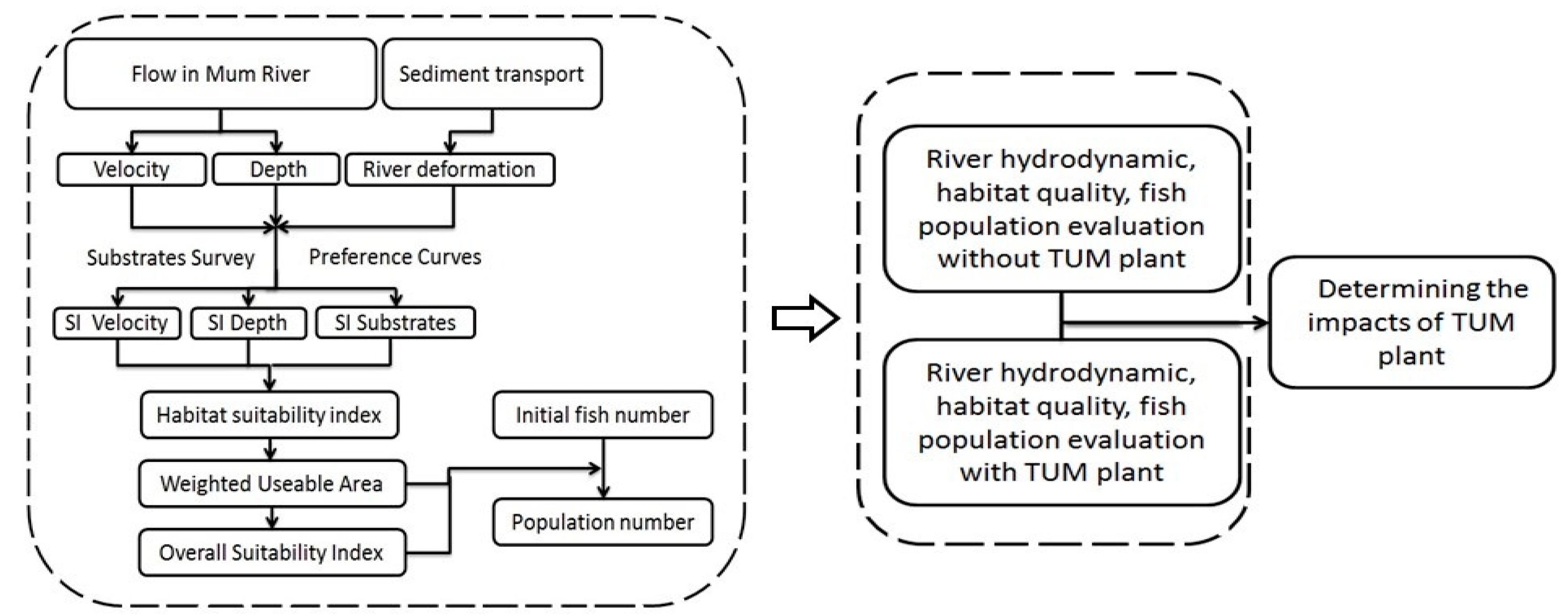
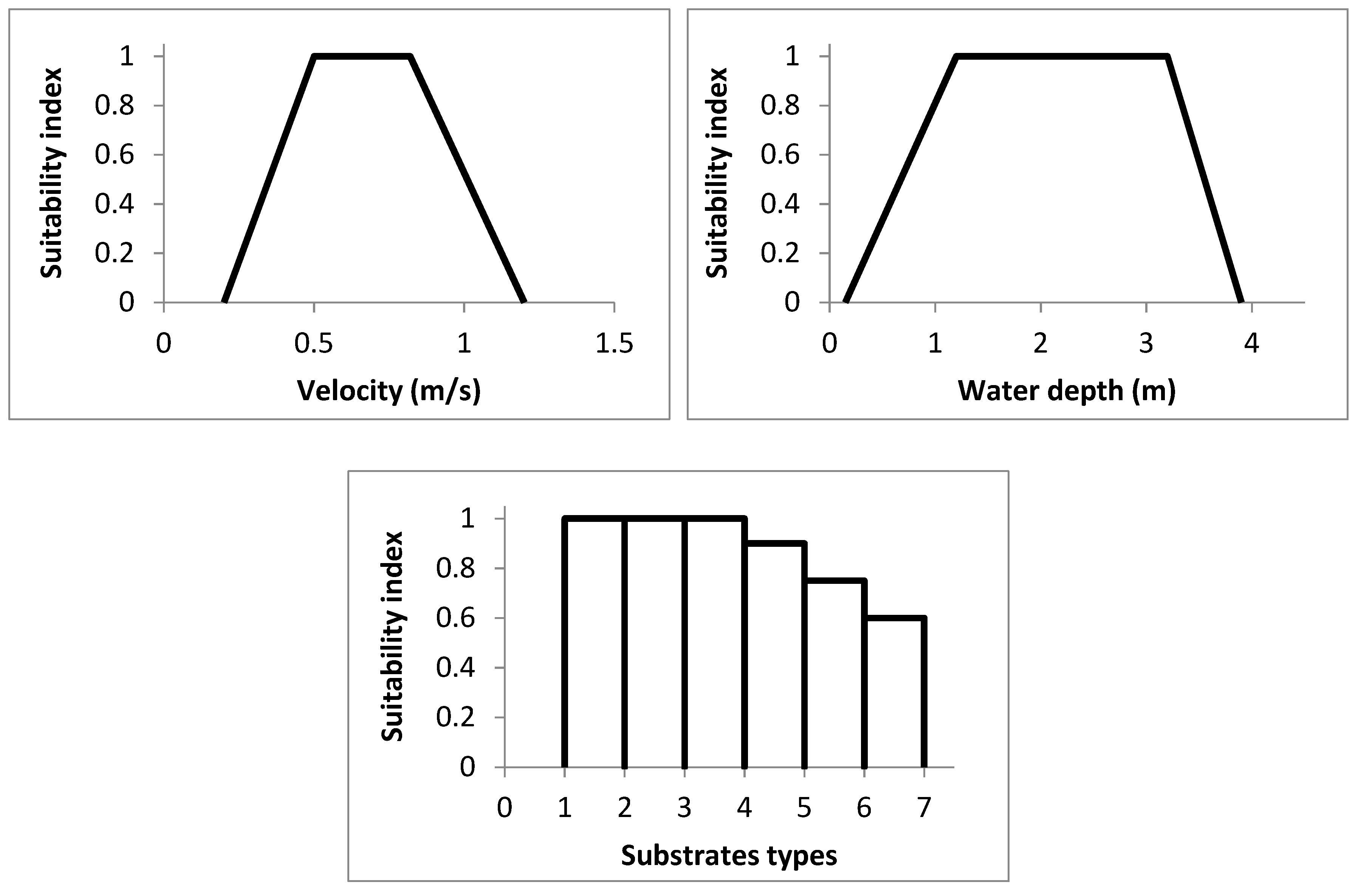
3.3. Habitat and Population Models

Habitat and population models were mainly composed by the habitat suitability index (HSI), the weighted usable area (WUA), the overall habitat suitability index (OSI), and the fish species number ( P t + 1 ). The HSI value was calculated for each mesh cell at each time step using the following equation:
H S I i , t = ( S I v × S I d × S I s ) 1 / 3
where S I v , S I d and S I s . are the suitability indices obtained from the fish preference curves (Figure 4). Only three important indices were selected for fish preference in this study: velocity, water depth, and river bed substrates. The preference curves of Black carp (Mylopharyngodon piceus) are showed in Figure 4, and were determined mainly from a literature review, field observations, and the professional judgment of ecologists [33,34].
The WUA was based on the distributions of habitat features in the computation domain. Based on the HSI values attributed to each mesh cell, the WUA was obtained by the following equation:
W U A t = i = 1 M A i H S I i , t
where Ai is the volume of mesh i (m2), and M is the number of meshes in the studied river. The overall suitability index (OSI) is determined by the following equation:
O S I = i = 1 M A i H S I i i = 1 M A i
The fish population calculation was converted from the logistic population model [60,61], and was developed by directly relating the results of the OSI and WUA in the habitat model using the following equation [44,45]:
P t + 1 = β × W U A t + 1 × P t × e α × ( O S I t + 1 χ ) β × W U A t + 1 + P t × ( e α × ( O S I t + 1 χ ) 1 )
where Pt and Pt+1 are the population numbers in the time steps t and t + 1; and α, β and χ are the model empirical parameters that were related to study the domain and fish species (in this study, α = 0.9, β = 2.1 and χ = 0.18).

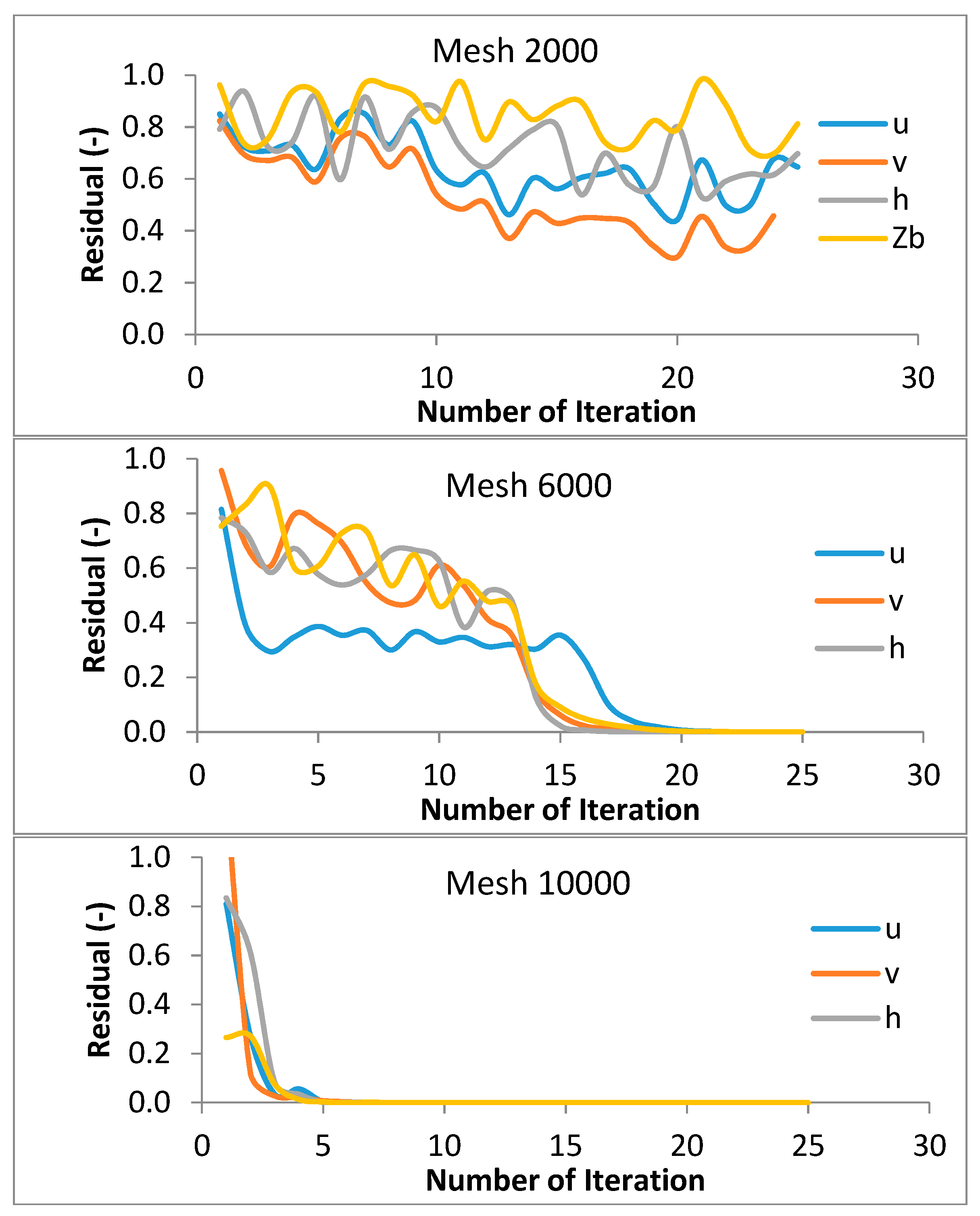
4. Numerical Methodology and Validation

To obtain the numerical results, the implicit finite volume method (FVM) was used to discretize the governing equations for flow and sediment transport with a curvilinear non-orthogonal grid. The turbulence model, bed deformation equation, and the sediment transport models were internally coupled with hydrodynamics. The convergence is guaranteed when the maximum residence of error is less than 10−9. To test the convergence of u, v, and h, a monitoring point was set with a maximum of 50 iterations. In this study, a grid independence test was conducted with meshes of grid resolutions of 2000, 6000 and 10,000. Through testing, the convergence criteria could be obtained when the mesh was 10,000 so a mesh of 13,994 (over 10,000) was selected as the final grid mesh resolution (Figure 5).
The initial and boundary conditions were set in both S1 and S2. The inlet was set by the flow rate versus time. In the outlet, the stage-discharge curve was set, and zero gradient outflow boundaries were adopted for the variables of velocity and turbulent kinetics. The solid wall boundary condition was applied on the side boundary condition.

5. Results

The Mum River terrain is shown in Figure 2 with 13,994 mesh and 26,524 nodes, which represents an area of 4750 m2. The Mum River was used to evaluate the effects of the TUM plant construction on flow velocity, water depth, fish habitat quality distributions, and fish population fluctuation. The sensitive analyses of fish hurting rates (0%, 5%, 10%, and 20%) by the TUM plant were also analyzed.

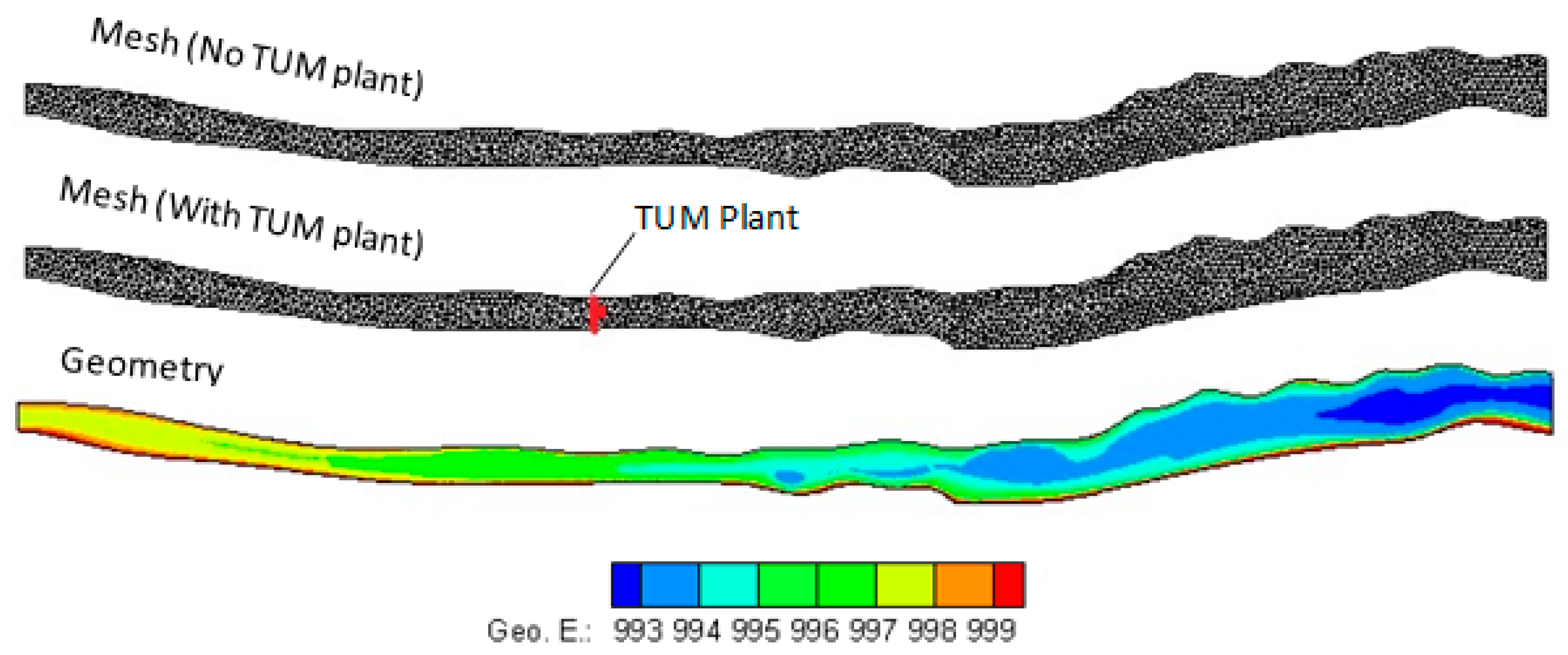
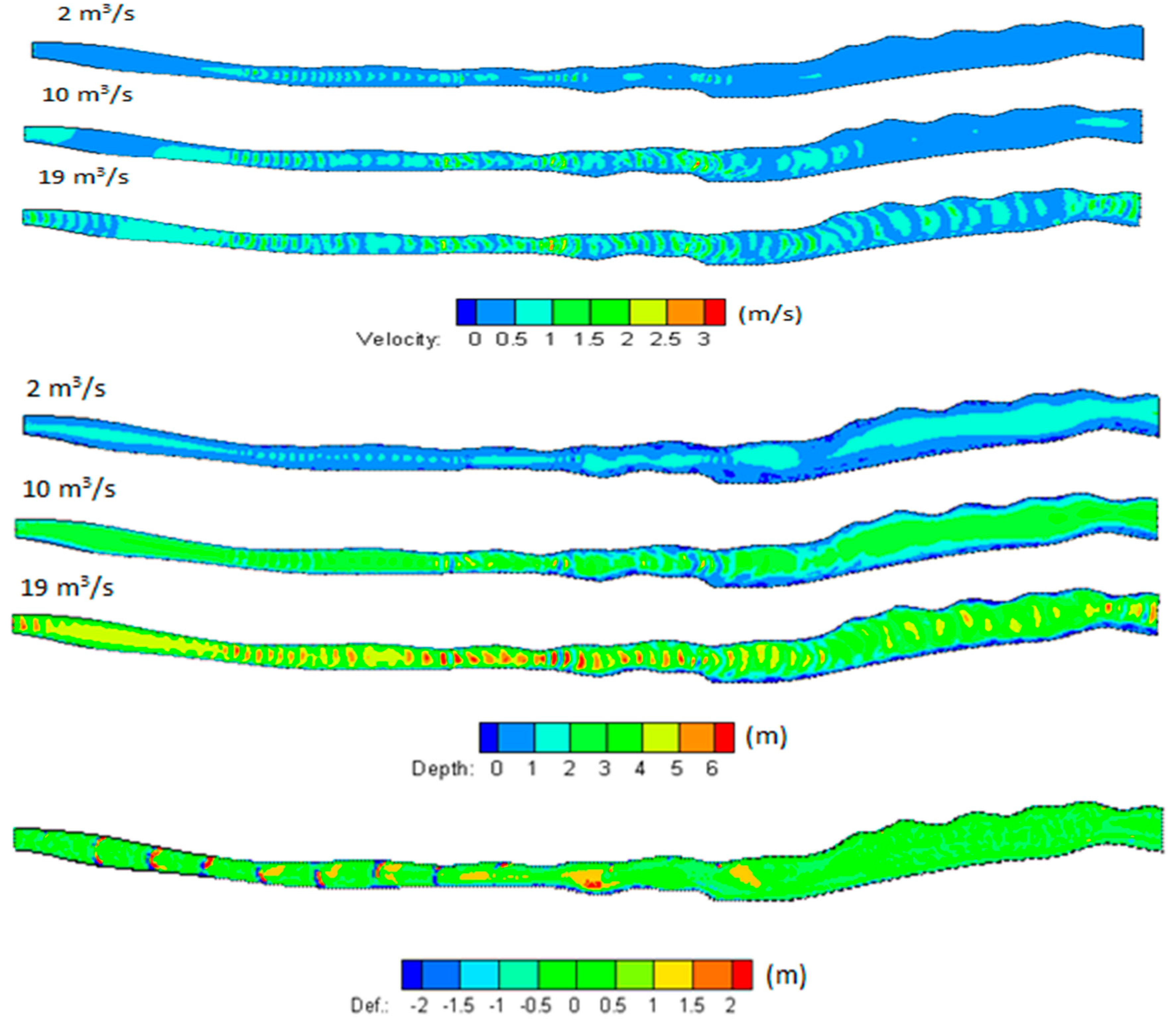
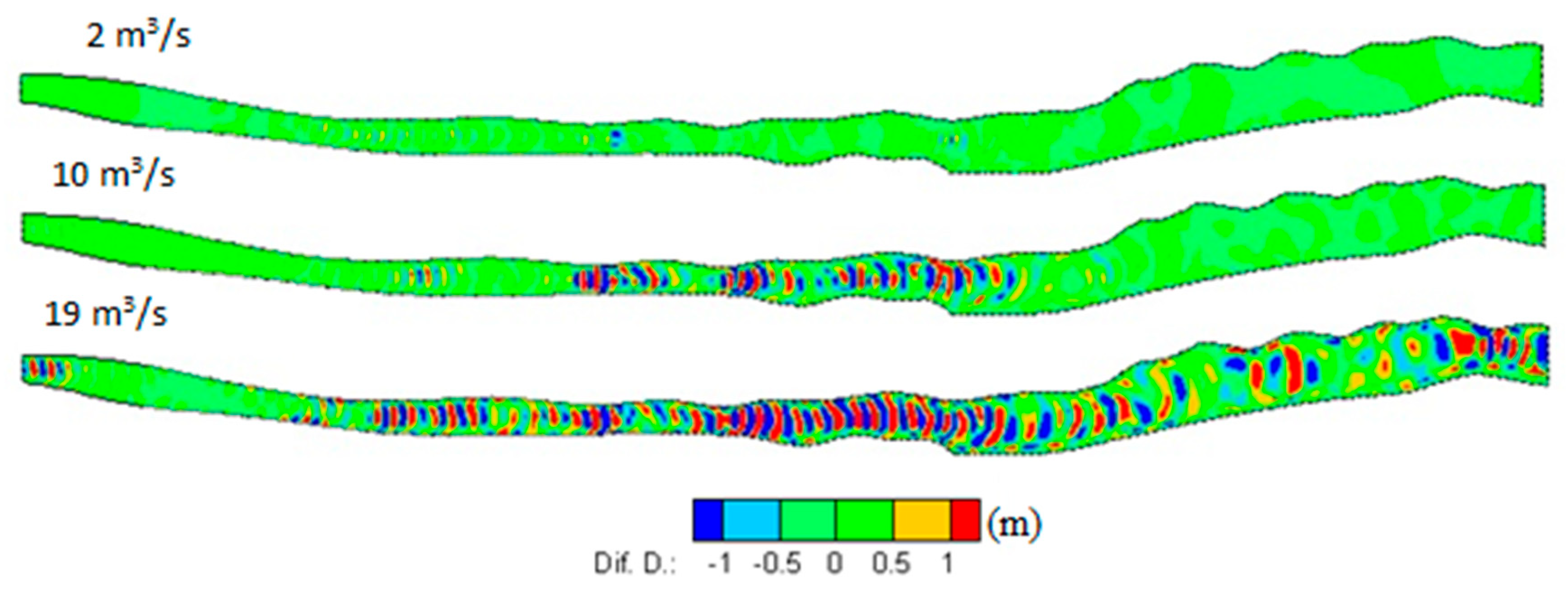
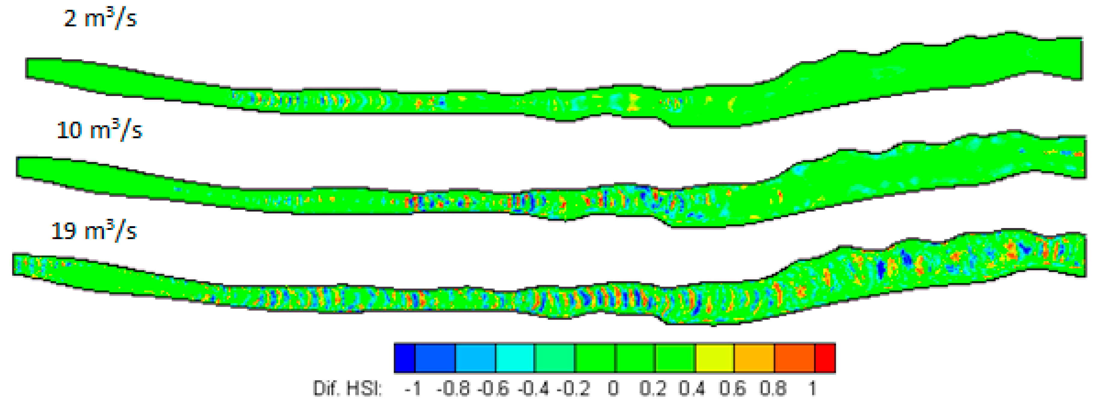
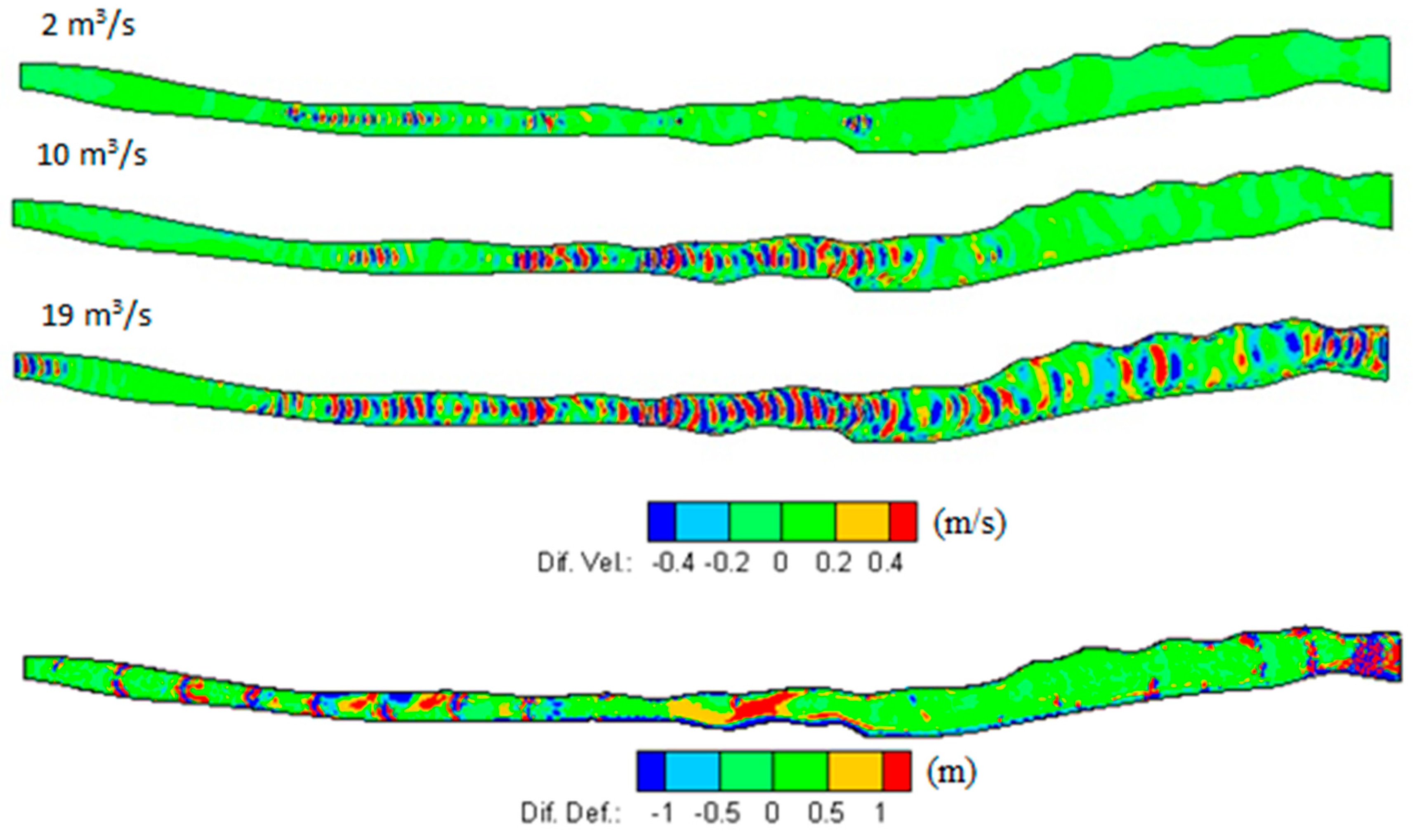
5.1. Velocity, Water Depth, and River Bed Deformation

Figure 6 indicates the velocity and water depth in the Mum River under discharges of 2 m3/s, 10 m3/s, and 19 m3/s. The simulation results revealed that the velocity in the calculation domain was 0.4 m/s to 0.8 m/s when the discharge was 2 m3/s. When the discharge increased to 10 m3/s, the velocity in the middle river stretch reached 1 m/s, which is much bigger than upstream and downstream of the river stretch. Unlike the velocity distribution pattern in 10 m3/s, the velocity distribution pattern in 19 m3/s started to become unstable at a maximum velocity of 2.6 m/s. The depth ranged from 0–1 m, 1–3 m, and 3.2–5.5 m for discharges of 2 m3/s, 10 m3/s, and 19 m3/s, respectively. Through simulation of the river bed deformation under average discharge, it was notable that during the simulation time, the largest scale deposition happened on the mid-length of the river stretch, with a maximum value of 1.8 m.

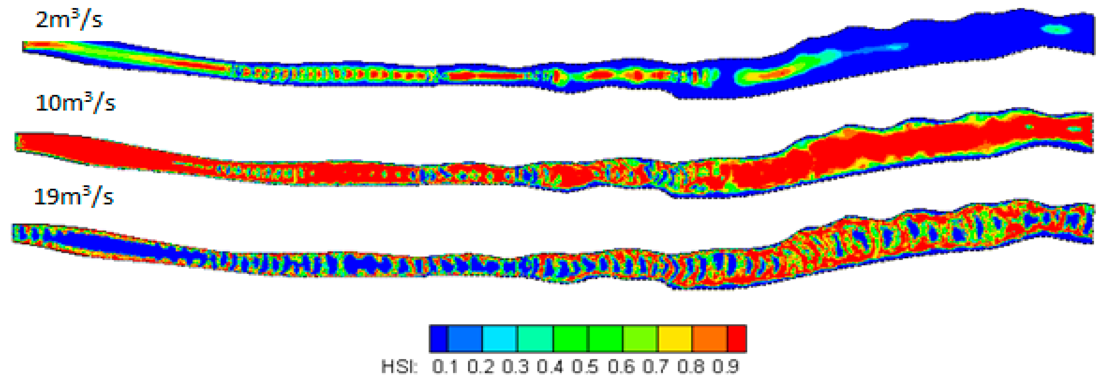
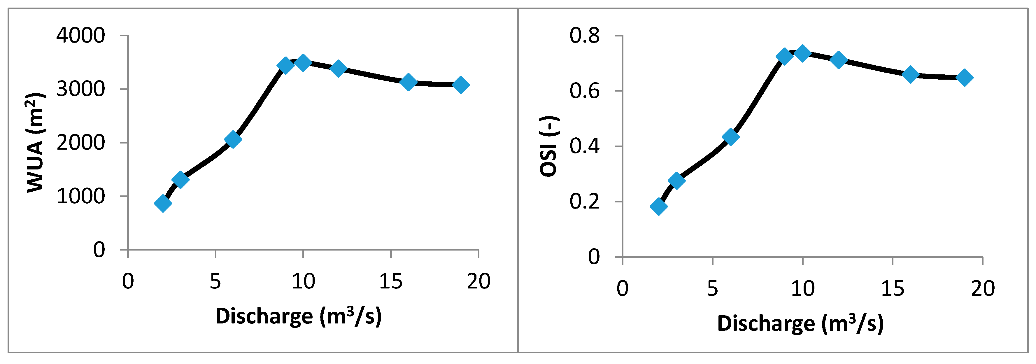
5.2. Habitat Suitability Index Distribution

The preference curves used to calculate the Mum River’s habitat quality and the simulation results are shown in Figure 7 and Figure 8. Figure 7 shows the HSI distribution under discharges of 2 m3/s, 10 m3/s, and 19 m3/s. When the discharge was 2 m3/s, the low HSI values were mainly located downstream of the river stretch due to the low water depth, and low velocity occurred downstream of the river stretch. A narrow strip area upstream and in the middle-stream had high HSI values, as the velocity overrides the role of the other parameters, and had a critical impact on the high HSI values. The HSI distribution trend became different when the discharge increased to 10 m3/s, with the high HSI values nearly filling the whole river stretch, and only a few very small areas upstream and in the middle-stream had low HSI values. When the discharge increased to 19 m3/s, the habitat quality in the majority of areas in the Mum River was still keep at a high level. However, the habitat quality at 19 m3/s was relatively low when compared with the habitat quality at 10 m3/s in the Mum River stretch.
The WUA and OSI were calculated from the HSI values based on Equations (8) and (9). The WUA and OSI values are shown in Figure 8, with discharges ranging from 2–19 m3/s. The simulation results indicate that the WUA and the OSI have the same trends. When the discharges increased from 2 m3/s to 10 m3/s, both WUA and OSI values showed increasing trends, with the WUA values increasing from 866 m2 to 3490 m2, and OSI values increasing from 0.18 to 0.74. However, when the discharges increased from 10 m3/s to 19 m3/s, both WUA and OSI values showed decreasing trends, with the WUA value decreasing from 3490 m2 to 3075 m2, and the OSI values decreasing from 0.74 to 0.65. The maximum values of WUA and OSI were 3490 m2 and 0.74, respectively.

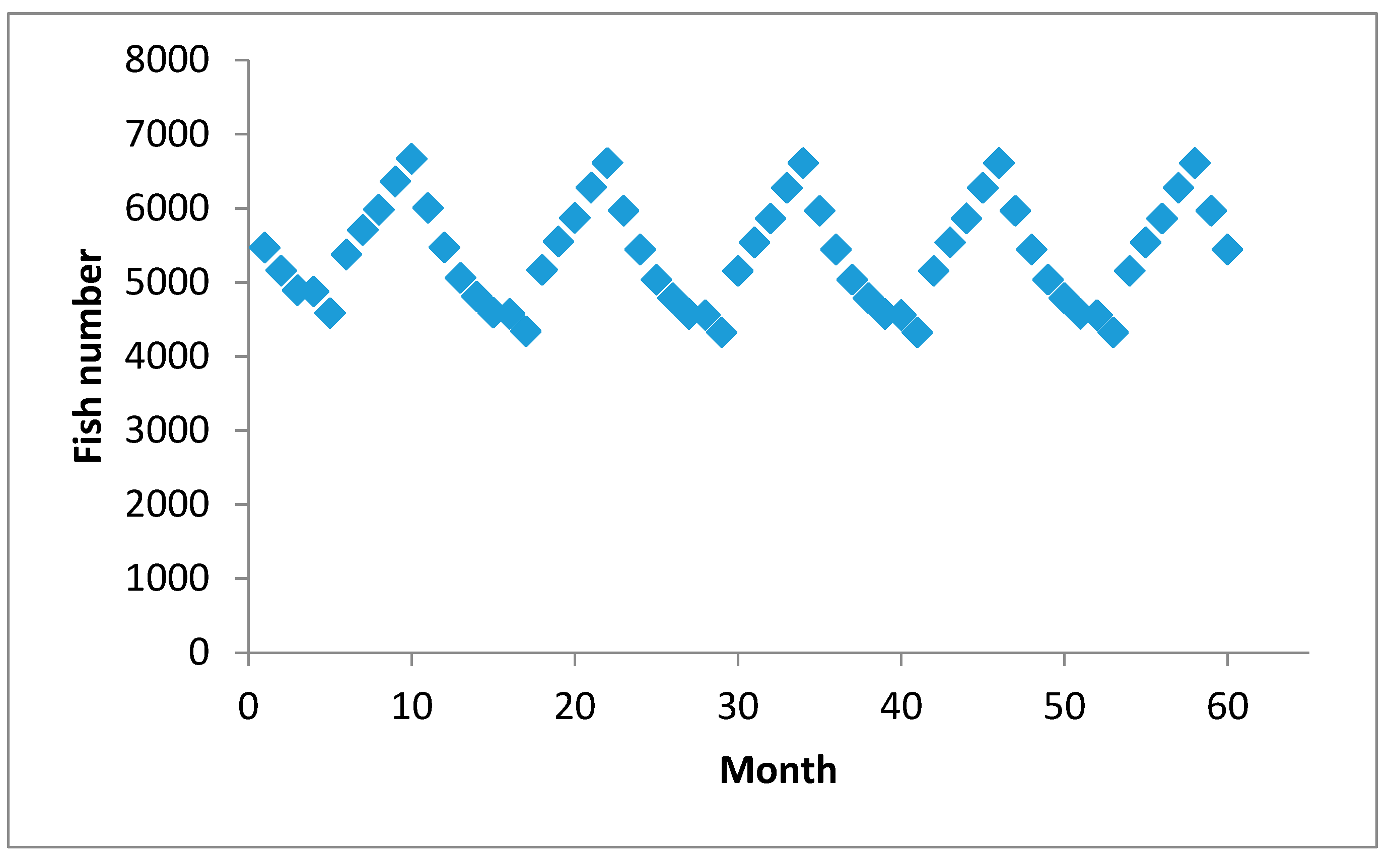
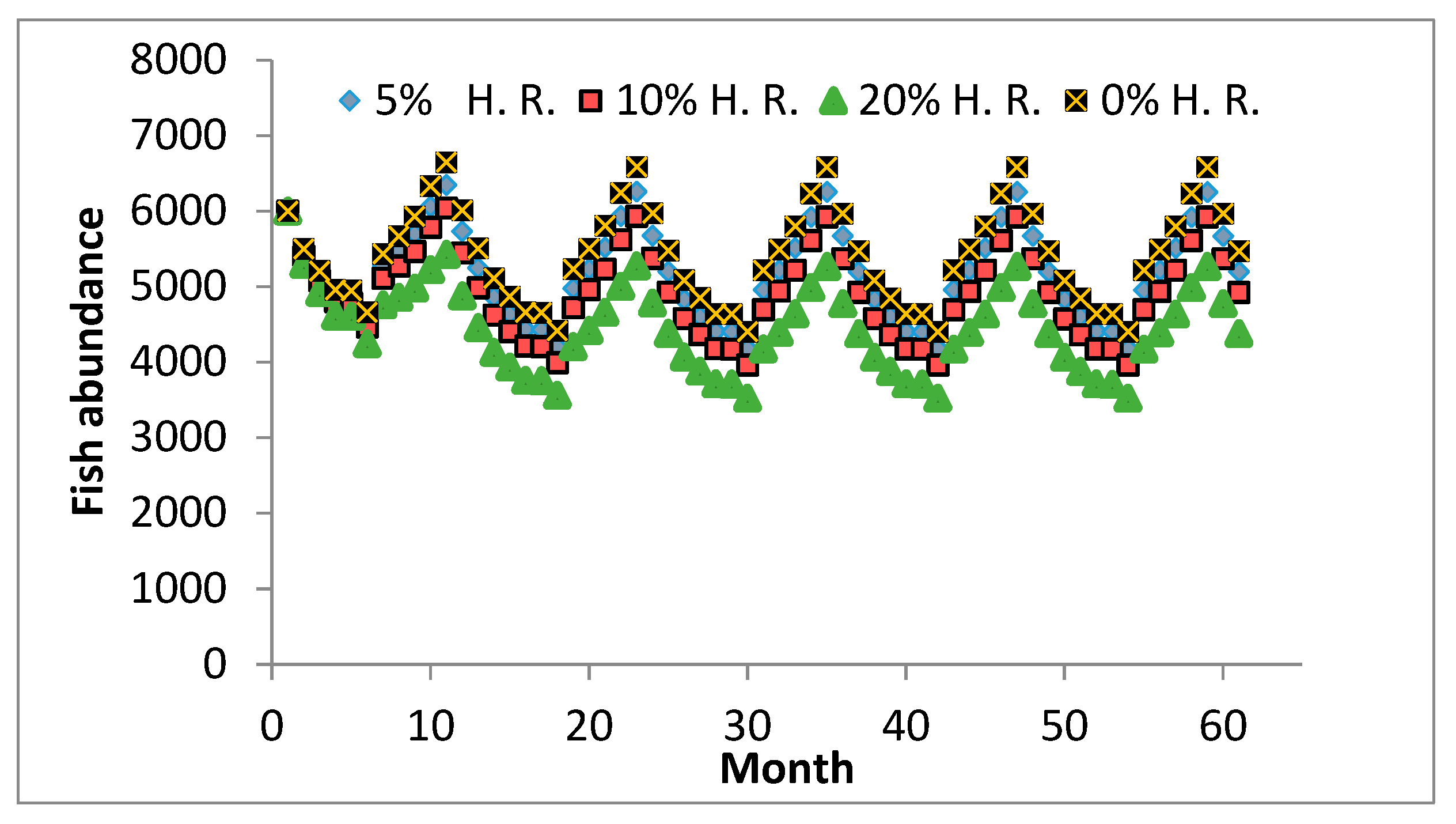
5.3. Fish Species Population Fluctuation

The fish abundance was defined as 6.0 × 10³ through a rough survey on the Mum River. A period of five years was considered for evaluating the fluctuation in the fish species population number. The predicted fish abundance fluctuation is shown in Figure 9, and the results indicate that the fish abundance periodically fluctuated with a maximum value of 6.6 × 10³ and a minimum value of 4.6 × 10³.

5.4. The Effects of the TUM Plant Construction

After the TUM plant was constructed on the Mum River, a series of comparisons have been made to determine the effects of the TUM plant on hydrodynamics, sediments, habitat qualities, and population numbers. Hydrodynamic and hydromorphology comparisons were made, and the results are shown in Figure 10. For hydrodynamic differences, the simulation results indicate that the velocity differences varied from −0.3 m/s to 0.3 m/s in the areas near the TUM plant when the discharge was 2 m3/s. The velocity differences varied from −0.5 m/s to 0.5 m/s for 10 m3/s, and −0.9 m/s to 0.9 m/s for discharges at 19 m3/s. Meanwhile, the water depth differences ranged from −0.4 m to 0.4 m and −0.6 m to 0.6 m for discharges of 10 m3/s and 19 m3/s, respectively. The river bed deformation differences for the majority areas of the river were not notable. The TUM plant only increased the erosion in the TUM plant tail water areas, which was due to the river bottom elevation difference upstream and downstream of the TUM plant. Through the comparison, it was notable that the TUM plant only affected 150 m along the Mum River: 50 m upstream and 100 m downstream of the plant. For the maximum discharge of the Mum River, the velocity and water depth differences varied drastically, and were due to the unstable flow velocities and depths, rather than the effects of the TUM plant.
After the TUM plant was constructed in the Mum River, the HSI, WUA, and OSI values were simulated. The HSI distribution comparisons between S1 and S2 in the Mum River are shown in Figure 11. When the discharge ranged from 2 m3/s to 16 m3/s, it was noted that the HSI values in the majority of areas were not affected by the TUM plant construction, with the exception of a small area near the TUM plant. When the discharge increased to 19 m3/s, the differences in HSI values between S1 and S2 became evident in the middle of the river and downstream. Figure 12 and Table 1 show that the differences in the WUA and OSI absolute values between S1 and S2 were very small when the discharge was lower than 16 m3/s. However, when the discharge increased to 19 m3/s, the differences of the WUA and OSI absolute values between S1 and S2 increased to 641 m2 and 13.5% for the WUA and OSI, respectively. The main reason for this big difference was due to the flow velocity and the depth becoming unstable in the river.
When considering the fish abundance fluctuations in the Mum River after the TUM plant construction, the fish injury rates by turbine need to be studied. In this study, four types of injury rates were considered: 0%, 5%, 10%, and 20%. The determination of injury rates was based on the testing guidelines of the physical model of the power plant. When the injury rate was 0%, the fish abundance had the same values as the fish abundance without considering the TUM plant. When the injury rates increased to 5%, 10%, and 20%, the fish abundance showed decreasing trends over the first three years, and then fluctuated regularly at a relatively stable level. Thus, the fluctuation of fish abundance ranged from 4.2 × 10³ to 6.2 × 10³ for a 5% injury rate, from 4.0 × 10³ to 5.9 × 10³ for a 10% injury rate, and from 3.5 × 10³ to 5.2 × 10³ for a 20% injury rate (Figure 13).

6. Discussion

6.1. Model System Advantage and Limitation

We aimed to look for conceptual links between the TUM hydropower turbine and Mum River using the ecohydraulic model. In doing so, we were able to better characterize how the TUM hydropower turbine’s ecological behavior changed along the Mum River. We found that the ecosystem aspects of the TUM plant designs performed well with regard to their effects on river hydrodynamics and sedimentation. These findings are consistent with physical approaches that test the ecological concept of the TUM hydropower turbine [62,63]. The modeling results shows that our ecohydraulic model has distinct novel aspects compared with earlier studies that primarily focus on habitat suitability quality. The ecohydraulic model provided a quantitative way to link river fluvial, habitat, and population, and evaluate the effect of the TUM hydropower turbine on small river ecology. In addition, the fish abundance distribution can also be more precisely used to indicate fish density in the river.
For the prediction result, the ecohydraulic model system may overpredict or underpredict the model output. The accuracy mainly depended on the accuracy of the model’s validation, boundary conditions, and empirical relations [55,56]. There has been progress using modeling and analytical approaches due to the advantage of producing full-scale predictions that are cost-efficient as well as time-efficient. Overall, the numerical model could potentially provide suitable conditions for successful fish habitat restoration.
It should be noted that there remain several aspects to consider in this study. First, there were only three suitable indices used in this study; other parameters such as the water temperature and oxygen concentration could also be included to improve resolution. In addition, whether the change of the headwater, interaction among fish species and other organisms (e.g., macroinvertebrates), and the migration of fish species upstream and downstream of the Mum River will affect the fish abundance or not need further investigation. Furthermore, the fish abundance on different season (e.g., fry, juvenile, adult, and spawning) may change significantly, which could also be considered in further study.

6.2. TUM Plant Hydro Concept Analysis

The TUM plant design is a new, simple, and cost-effective hydroconcept. The ecohydraulic model system is a new approach that can be applied to support ecological assessments. The concern regarding ecological–hydraulic issues is constantly rising, and the numerical simulation could allow for the qualitative prediction of fish habitat quality and fish population fluctuations affected by the construction of a TUM plant. Furthermore, the ecohydraulic model system could assist in protecting the river ecosystem, and help to operate the TUM plant efficiently. It is also worth noting that while the simulations in this study were specifically looking at the TUM plant on the Mum River, the ecohydraulic model system can be easily adapted to assess the effects of constructing TUM plants on other small river regimes, natural rivers, and the big channel in irrigation districts in China. It can also be helpful to determine which part of the river the TUM plant ought to be installed near in order to minimize its impact on the fish population. Since it is necessary to encourage low or negative ecological impact with high-energy production, our approach extends the existing ecohydraulic model from a habitat model to a population model, and demonstrates the advantages of the novel model. This model system could assist ecological impact assessment for small hydropower. Our findings also suggest that the TUM power plant need further study in regard to eco-friendly technology and integrated fish protection on the Mum River, especially in relation to fish bypass design testing.

7. Conclusions

In this study, aspects of the TUM plant and its ecological effects on the river and stream ecosystem were studied using an ecohydraulic model system. The ecohydraulic model system was initially used to evaluate the hydrodynamics, hydromorphology, and ecological levels of the Mum River without (S1) and with (S2) consideration of the TUM plant, respectively.
Through an assessment of the effects of the TUM plant construction and the fish injury rates in the Mum River, it can be said that the ecosystem aspects of the TUM plant designs are excellent with regard to their effects on river hydrodynamics and sedimentation. The results indicate that the TUM plant construction has had minimal effects on fish habitat quality, and the effects on fish abundance are also very limited. Thus, it is expected that the TUM plant, due to its simple, economic, and low-maintenance hydropower design, is an attractive proposal that could be used in many small streams and rivers to generate electricity. It can also be confidently said that the TUM plant is an eco-friendly device, which can keep the river close to natural conditions with minimal alterations to the hydrodynamics and the fish abundance in the river.

Author Contributions

Conceptualization, W.Y.; Methodology, W.Y.; Software, W.Y. and G.Y.; Validation, X.M., M.X. and F.L.; Data Curation, M.X.; Writing-Original Draft Preparation, W.Y.; Writing-Review & Editing, all authors; Funding Acquisition, W.Y., Y.C. and M.X. All authors have make contribution on this research articles. The authors also would like to thank for the helps and useful discussion from Chair of hydraulic and water resources engineering, Technical University of Munich.

Funding

This research was funded by National Key R&D Program of China (2016YFC0502004). National Natural Science Foundation of China (Nos. 41661144030; 41571009), CCA (2017.07), and CAS project (Y6V60222YZ).

Acknowledgments

The work was financially support by National Key R&D Program of China (2016YFC0502004), National Natural Science Foundation of China (Nos. 41661144030; 41571009), and CAS project (Y6V60222YZ). The authors also would like thanks for the Figure 1 authority.

Conflicts of Interest

The authors declare no conflict of interest.

References

  1. Yuksek, O.; Komurcu, M.I.; Yuksel, I.; Kaygusuz, K. The role of hydropower in meeting Turkey’s electric energy demand. Energy Policy 2006, 34, 3093–3103. [Google Scholar] [CrossRef]
  2. Gürbüz, A. The role of hydropower in sustainable development. History 2006, 20, 25-000. [Google Scholar]
  3. Twidell, J.; Weir, T. Renewable Energy Resources; Routledge: London, UK, 2015. [Google Scholar]
  4. Zarfl, C.; Lumsdon, A.E.; Berlekamp, J.; Tydecks, L.; Tockner, K. A global boom in hydropower dam construction. Aquat. Sci. 2015, 77, 161–170. [Google Scholar] [CrossRef]
  5. Penche, C. Guide on How to Develop a Small Hydropower Plant; European Small Hydropower Association (ESHA): Brussels, Belgium, 2014; 296p. [Google Scholar]
  6. Huang, S.; Chen, C.; Bai, Q.; Zheng, C. China hydropower current situation and future trends. Technol. Innov. Appl. 2016, 27, 204. [Google Scholar]
  7. Huang, H.; Yan, Z. Present situation and future prospect of hydropower in China. Renew. Sustain. Energy Rev. 2009, 13, 1652–1656. [Google Scholar] [CrossRef]
  8. Bhat, I.K.; Prakash, R. LCA of renewable energy for electricity generation systems—A review. Renew. Sustain. Energy Rev. 2009, 13, 1067–1073. [Google Scholar]
  9. Nguyen, T.H.; Everaert, G.; Boets, P.; Forio, M.A.; Bennetsen, E.; Volk, M.; Hoang, T.H.; Goethals, P.L. Modelling Tools to Analyze and Assess the Ecological Impact of Hydropower Dams. Water 2018, 10, 259. [Google Scholar] [CrossRef]
  10. Taele, B.M.; Mokhutšoane, L.; Hapazari, I. An overview of small hydropower development in Lesotho: Challenges and prospects. Renew. Energy 2012, 44, 448–452. [Google Scholar] [CrossRef]
  11. Okot, D.K. Review of small hydropower technology. Renew. Sustain. Energy Rev. 2013, 26, 515–520. [Google Scholar] [CrossRef]
  12. Höffken, J.I. A closer look at small hydropower projects in India: Social acceptability of two storage-based projects in Karnataka. Renew. Sustain. Energy Rev. 2014, 34, 155–166. [Google Scholar] [CrossRef]
  13. Cheng, C.; Liu, B.; Chau, K.W.; Li, G.; Liao, S. China’s small hydropower and its dispatching management. Renew. Sustain. Energy Rev. 2015, 42, 43–55. [Google Scholar] [CrossRef]
  14. Zhou, S.; Zhang, X.; Liu, J. The trend of small hydropower development in China. Renew. Energy 2009, 34, 1078–1083. [Google Scholar] [CrossRef]
  15. Paish, O. Small hydro power: Technology and current status. Renew. Sustain. Energy Rev. 2002, 6, 537–556. [Google Scholar] [CrossRef]
  16. Yi, M. There is great potential for small hydropower development in the world. China Water Electr. 2012, 9, 69. (In Chinese) [Google Scholar]
  17. Shang, S.; Gu, Z.; Cao, X. A review of hydropowerplant projects’ eco-hydraulic effects. Adv. Sci. Technol. Water Resour. 2014, 34, 14–19. [Google Scholar]
  18. Idsø, J. Small Scale Hydroelectric Power Plants in Norway. Some Microeconomic and Environmental Considerations. Sustainability 2017, 9, 1117. [Google Scholar] [CrossRef]
  19. Zhong, X.H. Degradation of ecosystem and ways of its rehabilitation and ways of its rehabilitation and reconstruction in dry and hot valley—Take representative area of Junsha river. Yunan Province as an example. Resour. Environ. Yangtza Basin 2000, 9, 376–383. [Google Scholar]
  20. Jackson, S.D. Ecological considerations in the design of river and stream crossings. In Proceedings of the International Conference on Ecology and Transportation, New York, NY, USA, 24–29 August 2003. [Google Scholar]
  21. Kibler, K.M.; Tullos, D.D. Cumulative biophysical impact of small and large hydropower development in Nu River, China. Water Resour. Res. 2013, 49, 3104–3118. [Google Scholar] [CrossRef]
  22. Parasiewicz, P. MesoHABSIM: A concept for application of instream flow models in river restoration planning. Fisheries 2001, 26, 6–13. [Google Scholar] [CrossRef]
  23. Huang, G.; Chen, Q.; Jin, F. Implementing eco-friendly reservoir operation by using genetic algorithm with dynamic mutation operator. In Life System Modeling and Intelligent Computing; Springer: Berlin/Heidelberg, Germany, 2010; pp. 509–516. [Google Scholar]
  24. Yao, W.; Rutschmann, P.; Bamal, S. Modeling of River Velocity, Temperature, Bed Deformation and its Effects on Rainbow Trout (Oncorhynchus mykiss) Habitat in Lees Ferry, Colorado River. Int. J. Environ. Res. 2014, 8, 887–896. [Google Scholar]
  25. Zhang, W.; Yao, W.; Li, L.; Zhang, Q. Using an Eco-hydrodynamic Model to Simulate the Impact of Trunk Dam Construction on Kraal River Fish Habitat and Community. Int. J. Environ. Res. 2016, 10, 227–236. [Google Scholar]
  26. U.S. Fish and Wildlife Service (USFWS). Habitat as a Basis for Environmental Assessment; USFWS, Report 101 ESM; USFWS: Fort Collins, CO, USA, 1980.
  27. Bovee, K.D. A Guide to Stream Habitat Analysis Using the Instream Flow Incremental Methodology; U.S. Fish and Wildlife Service: Washington, DC, USA, 1982.
  28. Bovee, K.D. Development and Evaluation of Habitat Suitability Criteria for Use in the Instream Flow Incremental Methodology; National Ecology Center, Division of Wildlife and Contaminant Research, Fish and Wildlife Service, US Department of the Interior: Washington, DC, USA, 1986; Volume 86.
  29. Ginot, V. EVHA, a Windows Software for Fish Habitat Assessment in Streams; Bulletin Francais de la Peche et de la Pisciculture: Lyon, France, 1995. [Google Scholar]
  30. Alfredsen, K.; Killingtveit, A. The habitat modelling framework: A tool forcreating habitat analysis programs. In Proceedings of the Second International Symposium on Habitat Hydraulics, Québec City, QC, Canada, 5–8 June 1996; pp. 215–227. [Google Scholar]
  31. Jorde, K.; Bratrich, C. Ecological evaluation of Instream Flow Regulations based on temporal and spatial variability of bottom shear stress and hydraulic habitat quality. In Proceedings of the 2nd International Symposium on Habitat Hydraulics, Ecohydraulics 2000, Quebec City, QC, Canada, 11–14 June 1996. [Google Scholar]
  32. Parasiewicz, P. The MesoHABSIM model revisited. River Res. Appl. 2007, 23, 893–903. [Google Scholar] [CrossRef]
  33. Wang, F.; Lin, B. Modelling habitat suitability for fish in the fluvial and lacustrine regions of a new Eco-City. Ecol. Model. 2013, 267, 115–126. [Google Scholar] [CrossRef]
  34. Zhang, W.; Zhao, L.; Yao, W.; Li, L. Optimization the operation of hydraulic dam for ecological flow requirement of You-Shui River due to the construction of hydropower stations. Lake Reserv. Manag. 2016, 32, 1–12. [Google Scholar] [CrossRef]
  35. Yao, W.; Kumar, V.; Rutschmann, P. Simulating dam effects on river deformation and rainbow trout (Oncorhynchus mykiss) population number. In Proceedings of the 7th River Flow 2014, Lausanne, Switzerland, 3–5 September 2014; pp. 2477–2483. [Google Scholar]
  36. Yao, W.; Bamal, S.; Rutschmann, P. Simulating High-Flow Effects (HFE) on river deformation and rainbow trout (Oncorhynchus mykiss) habitat. In Proceedings of the 7th River Flow 2014, Lausanne, Switzerland, 3–5 September 2014; pp. 2471–2476. [Google Scholar]
  37. Deangelis, D.L.; Gross, L.J. Individual-Based approach is most appropriate for a given problem? In Individual-Based Models and Approaches in Ecology: Populations, Communities, and Ecosystems; Chapman and Hall: New York, NY, USA, 1992; pp. 67–87. [Google Scholar]
  38. Grimm, V. Ten years of individual-based modelling in ecology: What have we learned and what could we learn in the future? Ecol. Model. 1999, 115, 129–148. [Google Scholar] [CrossRef]
  39. Hall, A.J.; McConnell, B.J.; Rowles, T.K.; Aguilar, A.; Borrell, A.; Schwacke, L.; Wells, R.S. Individual-based model framework to assess population consequences of polychlorinated biphenyl exposure in bottlenose dolphins. Environ. Health Perspect. 2006, 114, 60–64. [Google Scholar] [CrossRef] [PubMed]
  40. Harvey, B.C.; Jackson, S.K.; Lamberson, R.H. InSTREAM: The Individu-Al-Based Stream Trout Research and Environmental Assessment Model; US Department of Agriculture, Forest Service, Pacific Southwest Research Station: Albany, NY, USA, 2009; Volume 218.
  41. Bartholow, J.M.; Laake, J.L.; Stalnaker, C.B.; Williamson, S. A salmonid population model with emphasis on habitat limitations. Rivers 1993, 4, 265–279. [Google Scholar]
  42. Bartholow, J.M. Sensitivity of a salmon population model to alternative for-mulations and initial conditions. Ecol. Model. 1996, 88, 215–226. [Google Scholar] [CrossRef]
  43. Yao, W.; Rutschmann, P.; Bamal, S. Three High Flow experiment releases from Glen Canyon Dam on Rainbow Trout and Flannelmouth Sucker habitat in Colorado River. Ecol. Eng. 2015, 75, 278–290. [Google Scholar] [CrossRef]
  44. Yao, W.; Bui, M.; Rutschmann, P. Development of the ecohydraulic model system for assessing habitat and population status in freshwater ecosystems. Ecohydrology 2018. [Google Scholar] [CrossRef]
  45. Yao, W.; Chen, Y. Assessing three fish species ecological status in Colorado River, Grand Canyon based on physical habitat and population models. Math. Biosci. 2018. [Google Scholar] [CrossRef] [PubMed]
  46. Yao, W.; Chen, Y.; He, X. Glen Canyon Dam Operation Effects on Rainbow Trout Habitat and Population Status. Pol. J. Environ. Stud. 2018, 27, 1–12. [Google Scholar] [CrossRef]
  47. Yao, W.; Zhao, T.; Chen, Y.; Yu, G.; Xiao, M. Assessing the river habitat suitability and effects of introduction of exotic fish species based on anecohydraulic model system. Ecol. Inform. 2018, 45, 59–69. [Google Scholar] [CrossRef]
  48. Rutschmann, I.P.; Sepp, D.I.F.A.; Barbier, D.I.J. Das Schachtkraftwerk–ein Wasserkraftkonzept in vollständiger Unterwasseranordnung. In Wasserkraftprojekte; Springer Fachmedien: Wiesbaden, Germany, 2013; pp. 286–291. [Google Scholar]
  49. Martins, D.E.C.; Seiffert, M.E.B.; Dziedzic, M. The importance of clean development mechanism for small hydro power plants. Renew. Energy 2013, 60, 643–647. [Google Scholar] [CrossRef]
  50. Acreman, M.C.; Ferguson, A.J.D. Environmental flows and the European water framework directive. Freshw. Biol. 2010, 55, 32–48. [Google Scholar] [CrossRef]
  51. Sepp, A.; Rutschmann, P. Ecological hydroelectric concept shaft power plant. In Proceedings of the International Seminar on Hydro Power Plants, Vienna, Austria, 6–9 November 2014. [Google Scholar]
  52. Rutschmann, P.; Schäfer, S. Das Schachtkraftwerk—Konzept, Funktion und Betrieb. Wasserkr. Ener. 2015, 21, 32–39. [Google Scholar]
  53. Lucchetti, E.; Barbier, J.; Araneo, R. Assessment of the technical usable potential of the TUM Shaft Hydro Power plant on the Aurino River, Italy. Renew. Energy 2013, 60, 648–654. [Google Scholar] [CrossRef]
  54. Rutschmann, P.; Sepp, A.; Geiger, F.; Barbier, J. TUM shaft hydro power-efficient and ecological. WasserWirtschaft 2011, 101, 33–36. [Google Scholar] [CrossRef]
  55. Rodi, W. Turbulence Models and Their Application in Hydraulics; CRC Press: Boca Raton, FL, USA, 1993. [Google Scholar]
  56. Parker, G.; Paola, C.; Leclair, S. Probabilistic Exner sediment continuity equation for mixtures with no active layer. J. Hydraul. Eng. 2000, 126, 818–826. [Google Scholar] [CrossRef]
  57. Van Rijn, L.C. Sediment transport, part III: Bed forms and alluvial roughness. J. Hydraul. Eng. 1984, 110, 1733–1754. [Google Scholar] [CrossRef]
  58. Van Rijn, L.C. Sediment transport part I: Bed load transport. J. Hydraul. Eng. ASCE 1984, 110, 1431–1456. [Google Scholar] [CrossRef]
  59. Van Rijn, L.C. Principles of Sediment Transport in Rivers, Estuaries and Coastal Seas; Aqua Publications: Amsterdam, The Netherlands, 1993; Volume 1006. [Google Scholar]
  60. Russ, G.R.; Alcala, A.C. Marine reserves: Long-term protection is required for full recovery of predatory fish populations. Oecologia 2004, 138, 622–627. [Google Scholar] [CrossRef] [PubMed]
  61. Shepherd, J.J.; Stojkov, L. The logistic population model with slowly varying carrying capacity. ANZIAM J. 2007, 47, C492–C506. [Google Scholar] [CrossRef]
  62. Bratrich, C.; Truffer, B.; Jorde, K.; Markard, J.; Meier, W.; Peter, A.; Wehrli, B. Green hydropower: A new assessment procedure for river management. River Res. Appl. 2004, 20, 865–882. [Google Scholar] [CrossRef]
  63. Vaughan, I.P.; Diamond, M.; Gurnell, A.M.; Hall, K.A.; Jenkins, A.; Milner, N.J.; Naylor, L.A.; Sear, D.A.; Woodward, G.; Ormerod, S.J. Integrating ecology with hydromorphology: A priority for river science and management. Aquat. Conserv. 2009, 19, 113. [Google Scholar] [CrossRef]
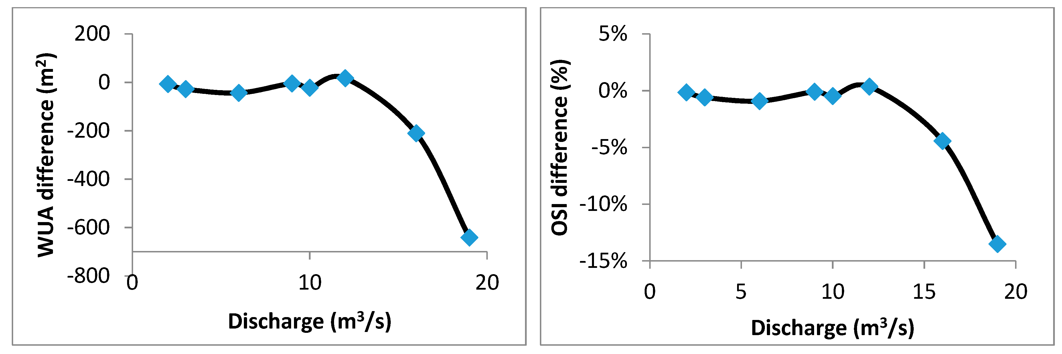
Figure 1. Prototype TUM plant at the Laboratory in Obernach (VAO).
Sustainability 10 01662 g001
Figure 2. River computational domains without the TUM shaft power plant and with the TUM shaft power plant (mesh) (Geo. E. = geometry elevation).
Sustainability 10 01662 g002
Figure 3. Flow chart of the ecohydraulic model system and the scenarios used in this study (SI = suitability index).
Sustainability 10 01662 g003
Figure 4. Fish preference curves for the fish species living in the Mum River (1 = Macrophytes; 2 = Clay (0.002–0.004 mm); 3 = Silt (0.004–0.062 mm); 4 = Sand (0.062–2 mm); 5 = Grave (2–64 mm); 6 = Cobblers (64–256 mm); 7 = Boulders (256–2048 mm)).
Sustainability 10 01662 g004
Figure 5. Comparison of the residual of u, v, h, and Zb in a monitoring point under three types of meshes (u, v = velocity at horizontal and vertical, respectively; h = water depth; Zb = river bed change).
Sustainability 10 01662 g005
Figure 6. Velocity, water depth, and sediment transport (one year) under the scenario without the TUM shaft power plant. Def: riverbed deformation.
Sustainability 10 01662 g006
Figure 7. Fish species habitat suitability index distributions under discharges of 2 m3/s, 10 m3/s, and 19 m3/s.
Sustainability 10 01662 g007
Figure 8. Weighted usable area (WUA) and overall suitability index (OSI) values under discharges from 2 m3/s to 19 m3/s.
Sustainability 10 01662 g008
Figure 9. Fish species abundance fluctuation for the scenario of no TUM plant on the Mum River.
Sustainability 10 01662 g009
Figure 10. Comparison of the differences of velocity, water depth and sediment transport between the scenario with the TUM plant and the scenario without the TUM plant (Dif. Vel. Is = difference of velocity; Dif. D. = difference of water depth; Dif. Def. = difference of deformation).
Sustainability 10 01662 g010aSustainability 10 01662 g010b
Figure 11. Habitat suitability index comparisons between the scenario without the TUM plant and the scenario with the TUM plant for discharges at 2 m3/s, 10 m3/s, and 19 m3/s (Dif. HSI = difference of habitat).
Sustainability 10 01662 g011
Figure 12. WUA and OSI difference under discharges ranged from 2–19 m3/s.
Sustainability 10 01662 g012
Figure 13. Fish population fluctuations under the power plant injury rates for fish: 0%, 5%, 10%, and 20% (H. R. = injury rates).
Sustainability 10 01662 g013
Table 1. WUA and OSI comparison for the scenario without the TUM plant and the scenario with the TUM plant under discharge between 2–19 m3/s.
Discharge (m3/s)WUA (%)OSI (%)
20.80.8
32.152.15
62.132.13
91.441.44
100.640.64
120.50.5
166.76.7
1920.8620.86

