A Hybrid Model Based on A Modified Optimization Algorithm and An Artificial Intelligence Algorithm for Short-Term Wind Speed Multi-Step Ahead Forecasting


Abstract
:1. Introduction
- (1)
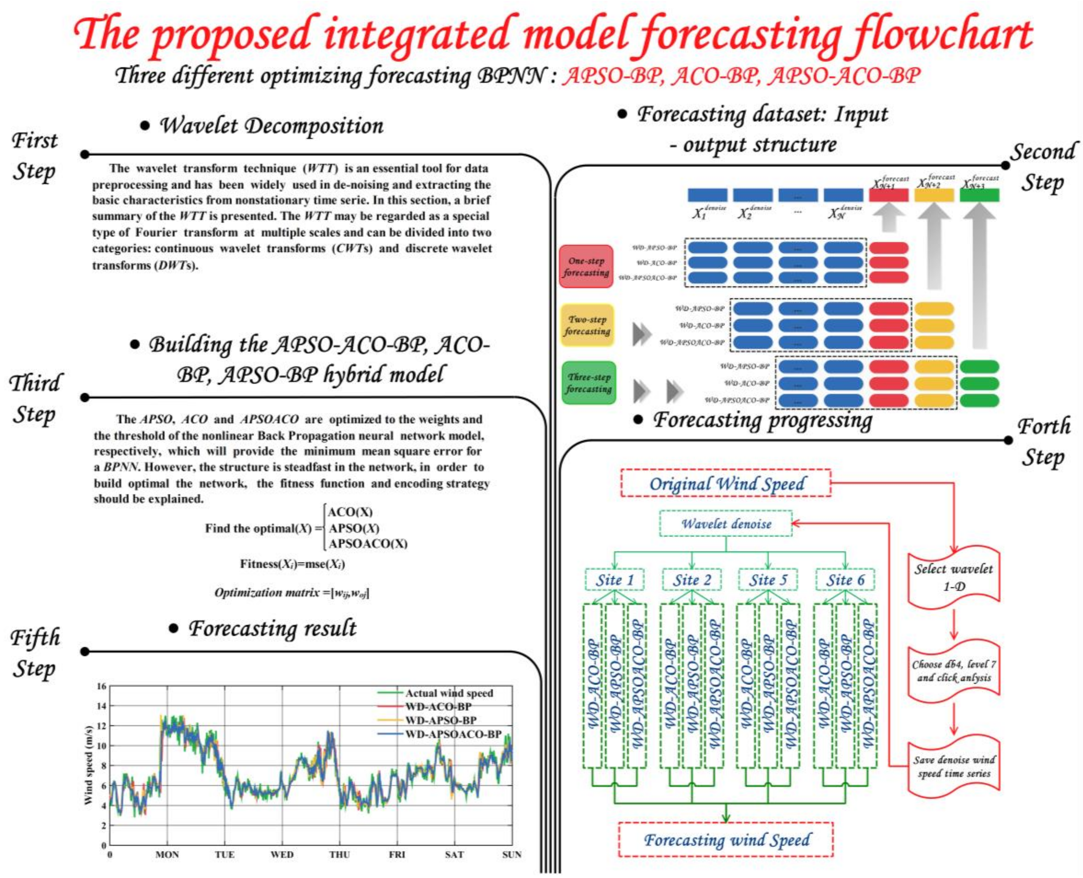
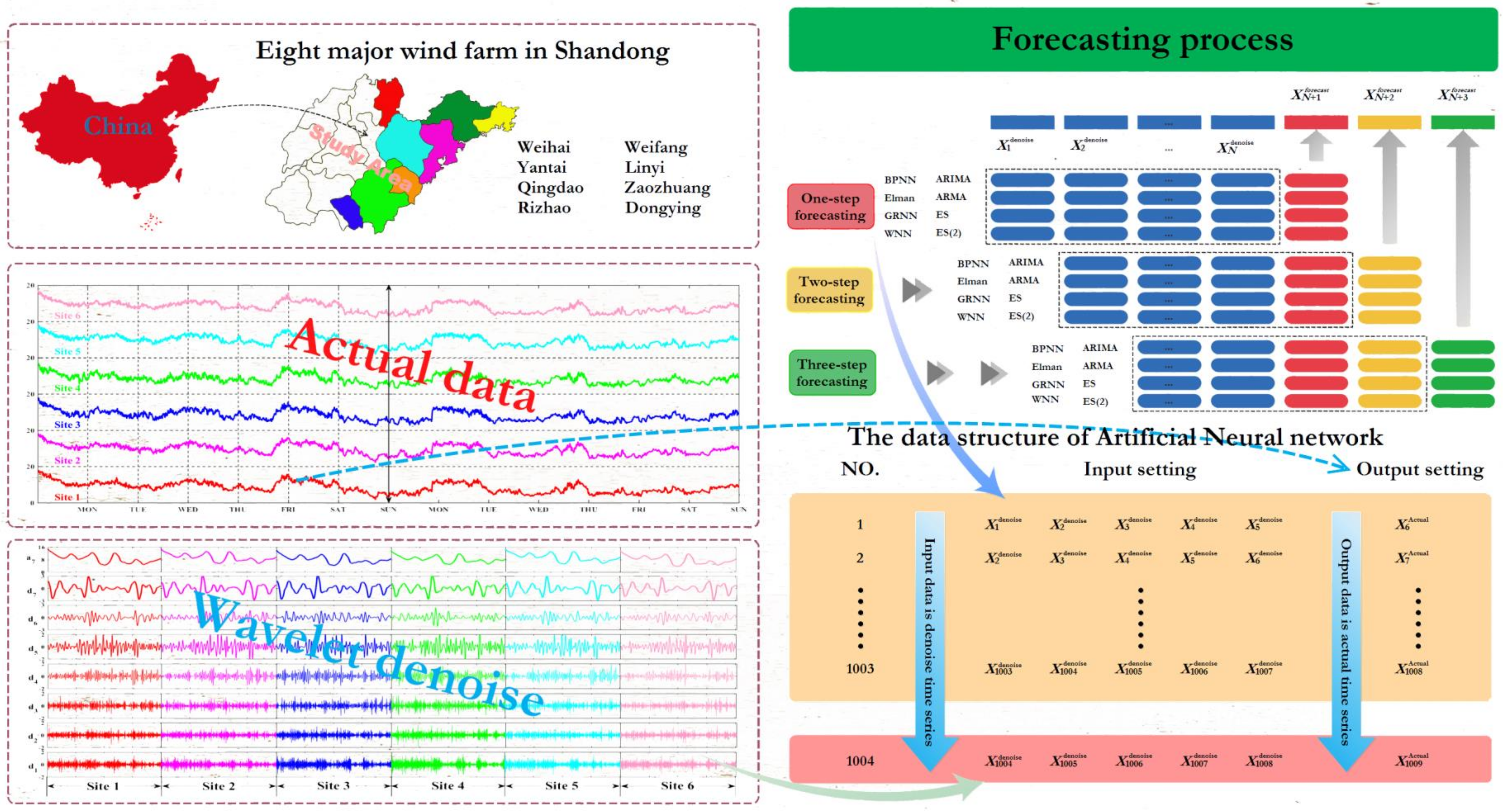
- Given that the wind speed exhibits uncertainty and randomness, a valid mathematical data preprocessing module, which was derived from the theory of signal time-frequency localization, is adopted to decompose the original wind speed time series into a number of sub-series. This module can effectively de-noise and fully extract the main features of a wind speed time series thus improves the forecasting accuracy.
- (2)
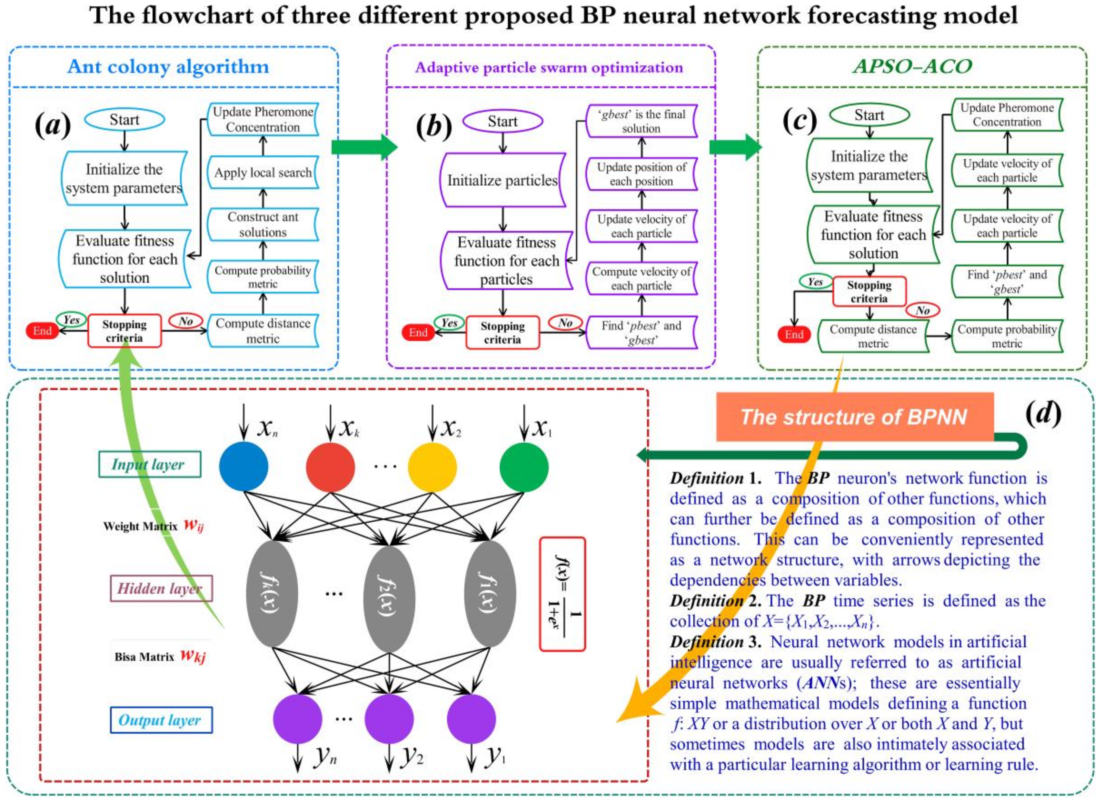
- A novel modified optimization algorithm, the APSOACO, is proposed to optimize the initial weights and thresholds of the BP neural network, due to its better convergence performance and lower number of required iterations compared with individual traditional optimization algorithms. This module not only provides a new option for solving problems such as computational complexity and easy trapping into a local optimal solution that traditional forecasting engines may encounter also makes a contribution to improving the accuracy of wind speed forecasting.
- (3)
- In order to estimate the overall performance of the developed hybrid model, a more scientific and comprehensive evaluation module is developed in this paper. This module not only sufficiently analyzes both the accuracy and stability of forecasting results also discusses the effectiveness of the proposed model in terms of the performance of the employed optimization algorithm and wavelet function.
- (4)
- With the aim of improving the quality of wind speed data and further enhancing the forecasting accuracy, an effective data interpolation technique and a rolling mechanism were also adopted in this paper. These techniques possess the capacity to enrich and improve the information of wind speed observations, which can in turn provide more accurate and stable wind speed forecasting.
2. Methodology
2.1. The Wavelet De-Noise Technique
2.2. The Artificial Neural Network Model and Fractal Representation
2.3. Fractal Interpolation
2.4. Rolling Mechanism Based Multi-Step Forecasting
- (a)
- 1-step ahead forecasting: The forecasting value is calculated based on the historical values, where N is the sample of training.
- (b)
- 2-step ahead forecasting: The forecasting value is calculated based on the historical values and the previous forecasting value .
- (c)
- 3-step ahead forecasting: The forecasting value is calculated based on the historical values and the previous forecasting value {, }.
2.5. Adaptive Particle Swarm Optimization
3. Back Propagation Neural Network Optimized by Hybrid Optimization Algorithm
3.1. Modified Ant Colony Optimization
3.2. Three Different Heuristic Algorithms for Optimizing BP Neural Network
4. Simulation Experimentation and Forecasting Result
4.1. Study Area and Data Description
4.2. Evaluation Criteria of Forecasting Performance
4.3. Experimental Process
4.4. The Experiment Preparation: Data Preprocessing
4.5. Structure of the Proposed Forecasting Framework
4.6. Experiment I: Selection of the Wind Speed Forecasting Model
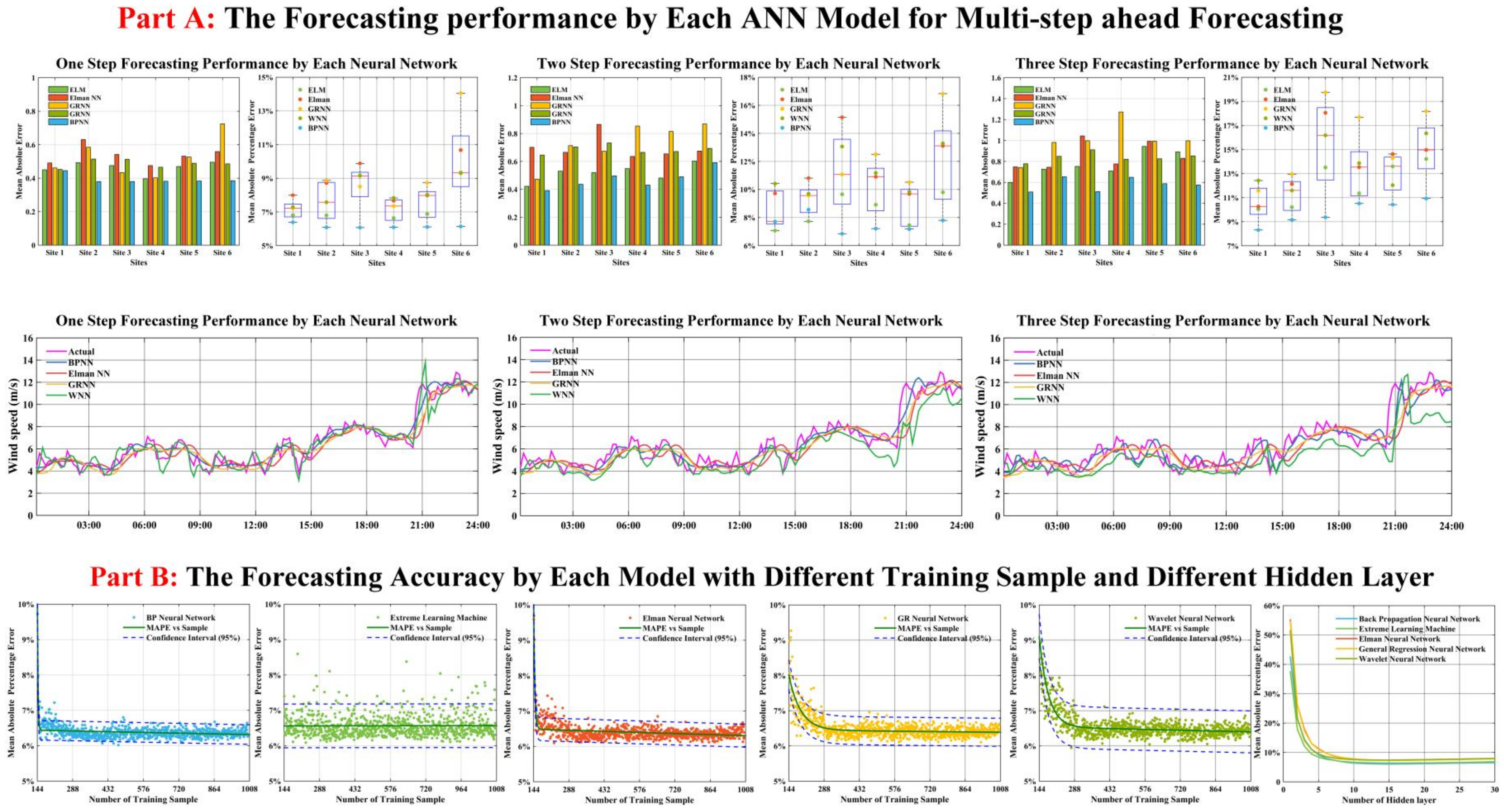
- (1)
- Table 3 shows the range of the input layer of each neural network is 3–8. With an increasing number of hidden layers, the test accuracy is gradually improved. When the number of hidden layers reaches a certain maximum number, the test accuracy is no longer improved.
- (2)
- Figure 3B shows that with an increase in the number included in the training sample, the fluctuation of testing accuracy reduces. For example, the confidence intervals obtained by the MAPE of the BP neural network is narrower than in the other four kinds of neural networks.
4.7. Experiment II: Comparison of Three Optimization Algorithms to Fine-Tune the Parameters of Hybrid Model
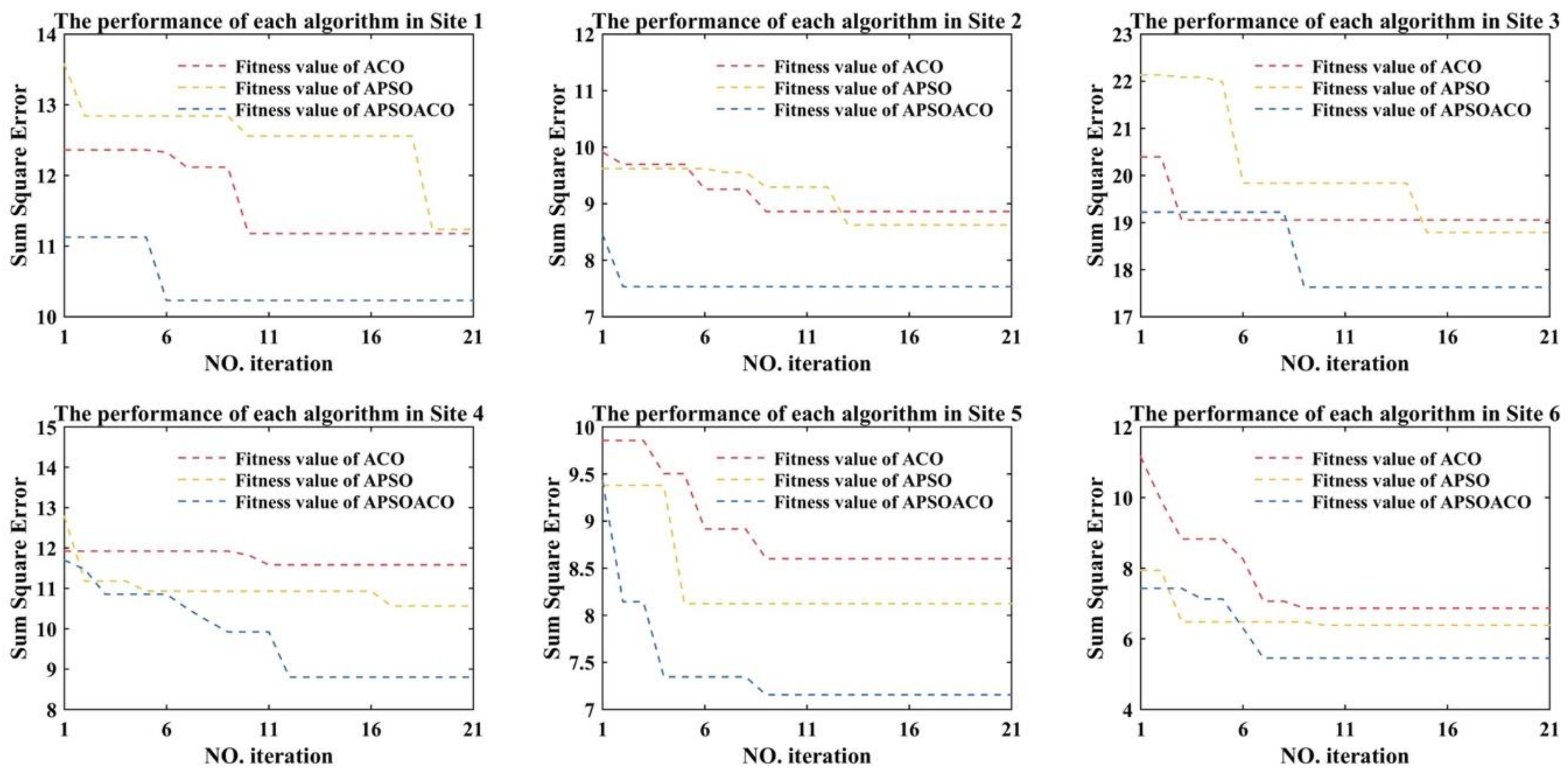
- (1)
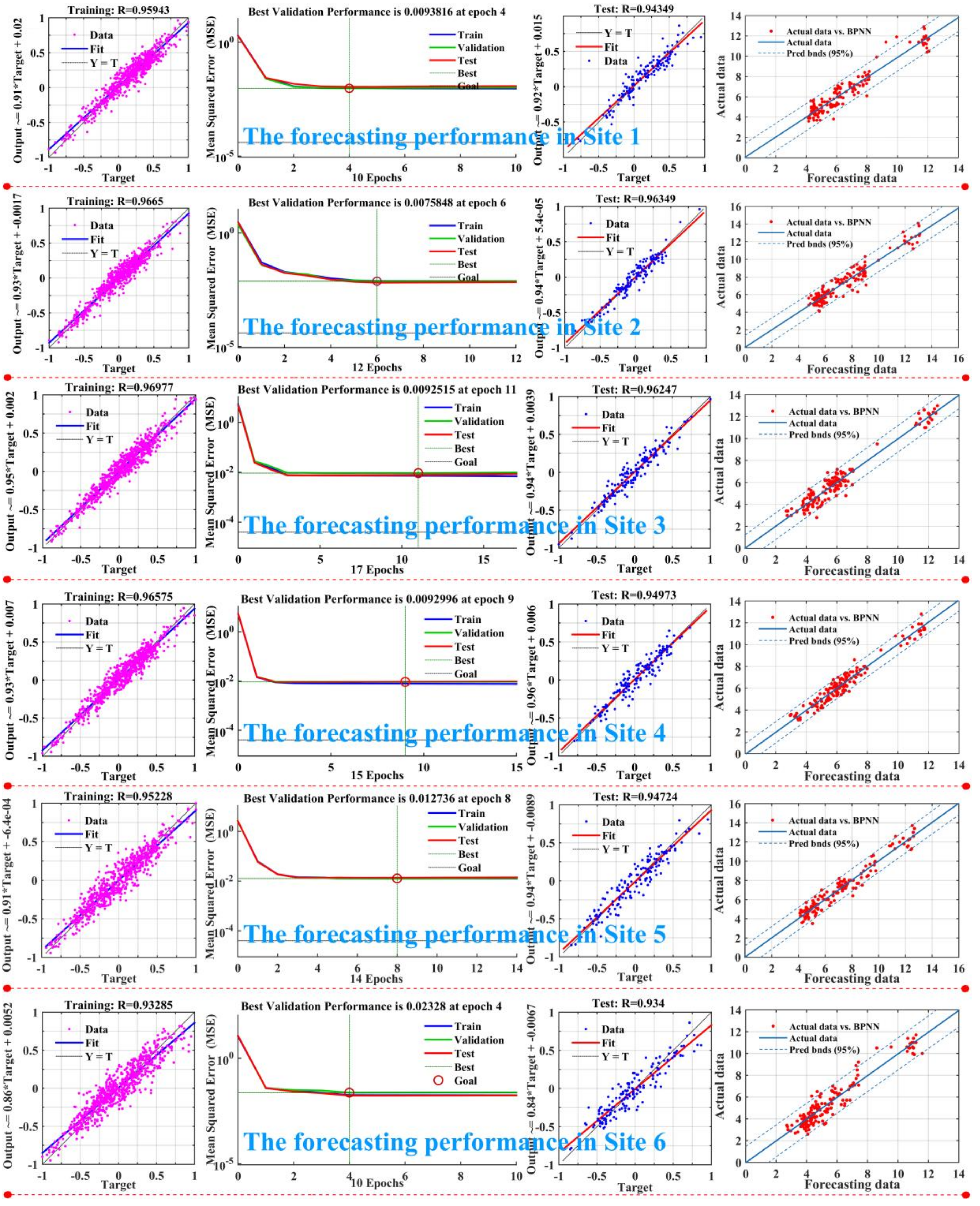
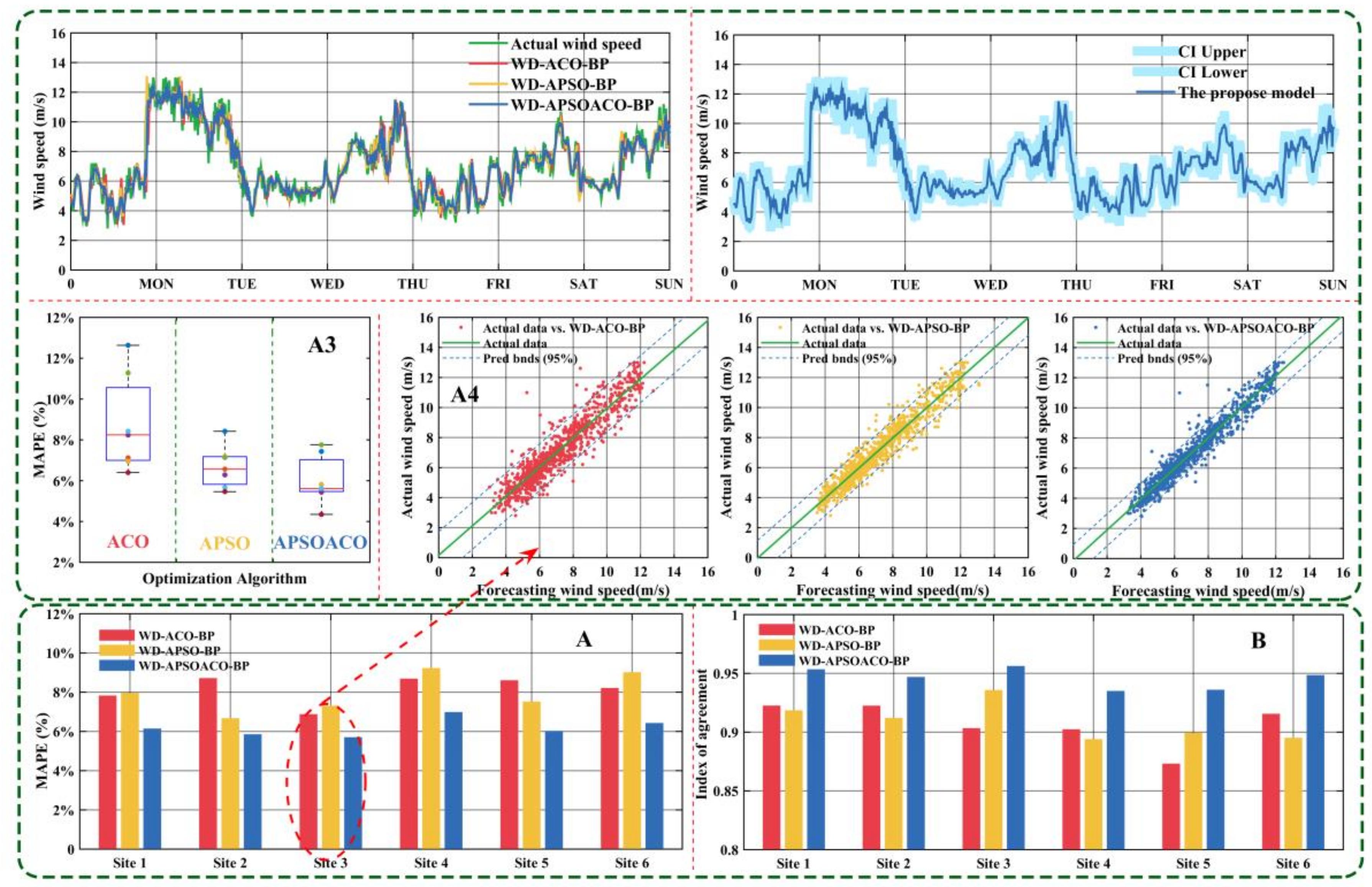
- It is noted that ACO suffers from slow convergence with increasing iterations. If the APSO algorithm falls into the local optimal points the capacity of the parameter optimization will be affected. The APSOACO algorithm combines the global search abilities of ACO with the local search capability of APSO, which significantly improves the parameter optimization ability of the single optimization algorithm. The numerical experimentation results indicate that the proposed hybrid model (WD-APSOACO-BP) outperforms the other hybrid models (WD-APSO-BP and WD-ACO-BP) when compared with the MAE, MSE, MAPE, the variance of MAPE, IA from Site 1 to Site 6. As such, the MAPE values of the WD-APSOACO-BP are 4.592%, 4.045%, 5.021%, 4.891%, 4.214%, 5.234%, corresponding to the Bias2 values which are 1.4400, 1.1852, 1.2405, 1.0029, 1.1860 and 1.3891 from Site 1 to Site 6, respectively. The WD-APSOACO-BP model can obtain higher forecasting accuracy than two single hybrid models. However, the IA values are 0.9619, 0.9627, 0.9456, 0.9584, 0.9545, 0.9456 from Site 1 to Site 6, which demonstrates that the WD-APSOACO-BP can achieve a better forecasting performance than the other hybrid models. Thus, the WD-APSOACO-BP can precisely forecast the future changes of a wind speed time series.
- (2)
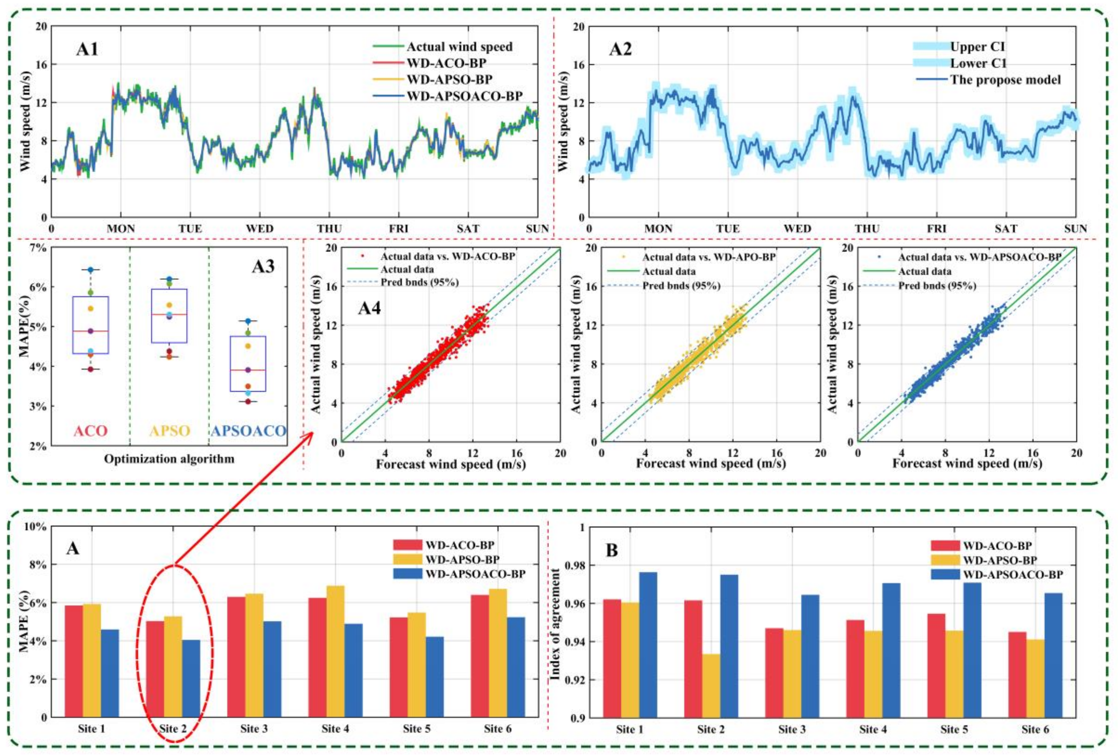
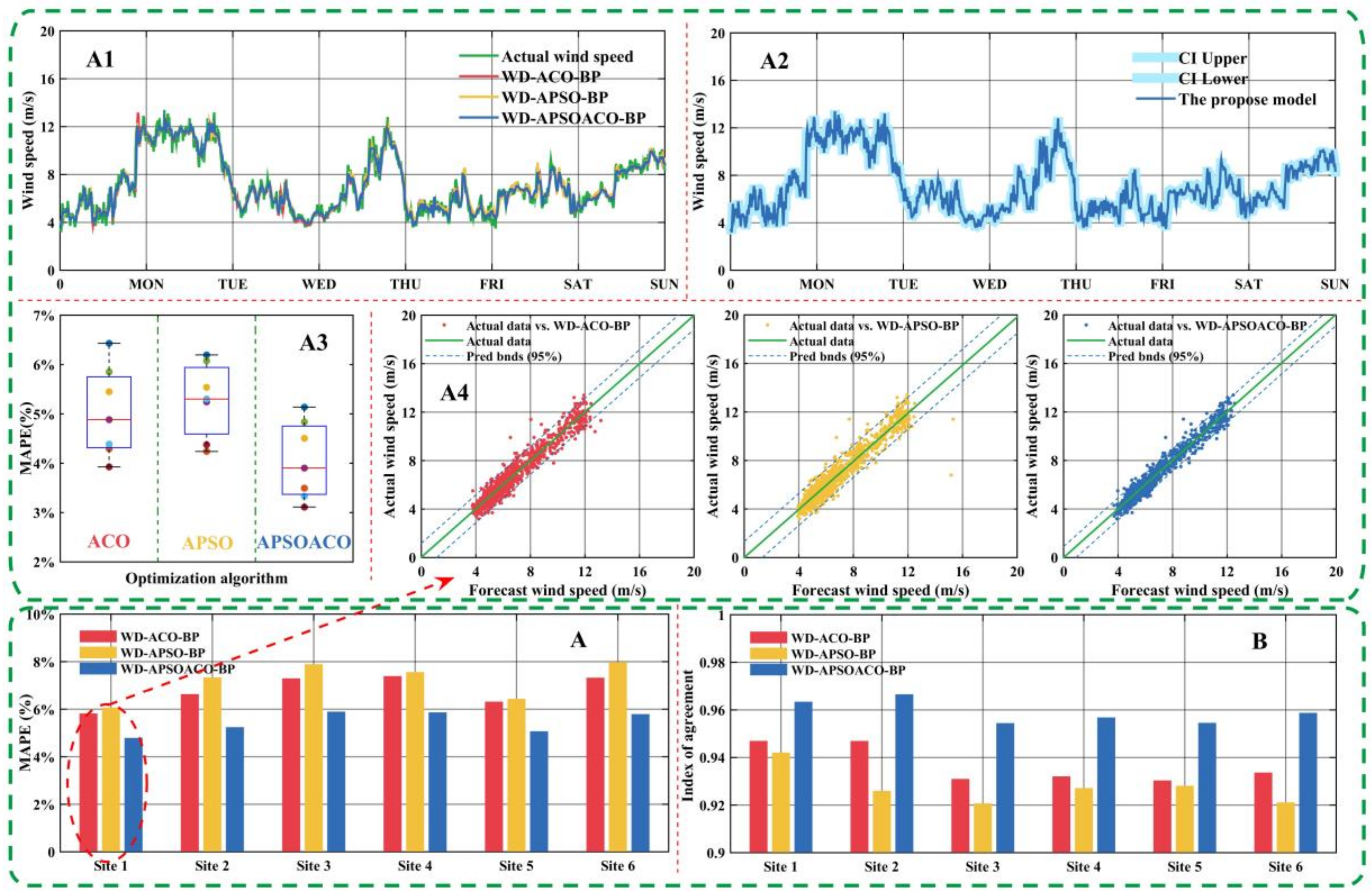
- With regards to further analysis of the forecasting results in terms of each day (the testing sample from Monday to Sunday), Table 5 and Figure 6A1–A4 clearly depict the forecasting values for 0:10 a.m. to 24:00 p.m., from 12 to 18. Part A and B of Figure 6 demonstrate the MAPE and IA from Site 1 to Site 6. The MAPE and IA of WD-APSOACO-BP are the minimum and the maximum, respectively. Part A1 of Figure 6 demonstrates the forecasting results of three different hybrid models and the actual wind speed series from 0:10 a.m. to 24:00 p.m., from 12 to 18 January 2014. Part A2 of Figure 6 demonstrates the 95% confidence intervals (CI) obtained by the WD-APSOACO-BP model. It can be clearly seen that both the upper CI and the lower CI are very close to the actual wind speed time series for Monday. Part A3 of Figure 6 is the Box-Plot of the MAPE from 0:10 a.m. to 24:00 p.m., over the course of a week, from 12–18 January, for the three hybrid models for Site 2. It can be seen that the performance of the WD-APSOACO-BP is better than that of the other two hybrid models. In addition, A4 clearly displays the actual wind speed time series compared with the forecasting results. It is obvious that the forecasting results offered by the proposed WD-APSOACO-BP method are very approximate to the target.
4.8. Experiment III: Comparison Three Different Hybrid Models in Multi-Step Ahead Wind Speed Forecasting
- (1)
- Table 6 shows the forecasting performance for each site of the three different hybrid models in 2-step forecasting in terms of six criteria: MAE, MSE, MAPE, Bias2 VAR(Y), and IA. For 2-step ahead forecasting, the proposed hybrid model outperforms the other hybrid models based on each of the evaluation criteria. For example, at Site 1, the proposed hybrid model provides a minimum forecasting error with MAE, MSE, MAPE values of 0.3490, 0.2135 and 4.79%, respectively. The IA and Bias2 achieved by this hybrid model are 0.9456 and 1.1183, respectively. Compared with the 2-step ahead forecasting achieved by the other hybrid models, the forecasting performance of the proposed hybrid model is still superior.
- (2)
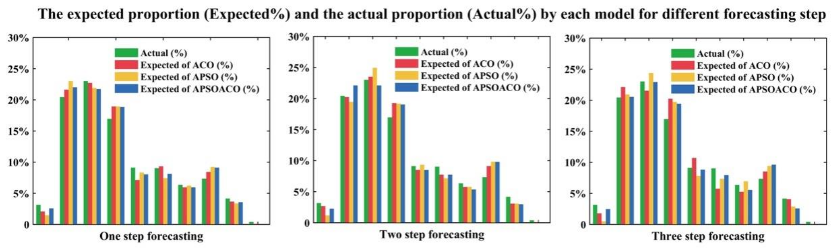
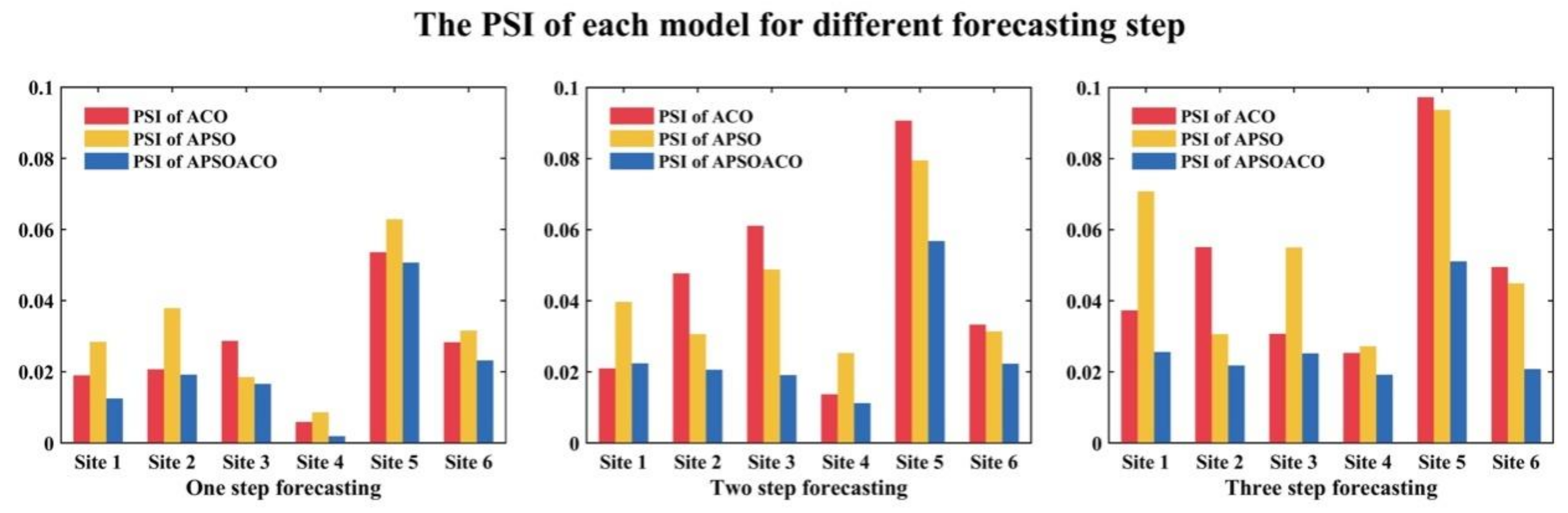
- Table 7 aims to evaluate the forecasting accuracy and stability of the proposed hybrid model in 3-step forecasting. The criterion in terms of evaluating the accuracy is the minimum MAPE values in the 1008 times experiments. This was selected to compare the accuracy of the three different hybrid models. The Bias2 values of the 1008 times experiments are utilized for the stability test. In terms of the accuracy testing, the WD-APSOACO-BP obtains a lower MAPE value than the other hybrid models. The Bias2 values of the proposed hybrid model always remains the lowest of the hybrid models. The proposed hybrid model obtains satisfactory forecasting stability and accuracy. In terms of the value of MAPE, the proposed hybrid model has the lowest value of MAPE among the three hybrid models. For 3-step forecasting at six sites, the proposed hybrid model obtains the smallest values of Bias2 compared to the other two hybrid models.
5. Discussion
5.1. Discussion the Forecasting Accuracy of the Model
5.2. Verification Stability of Forecasting Results
5.3. Analysis of the Optimization Performance of Hybrid Optimization Algorithm
- (1)
- The inspired factor has large influence on the optimization performance and convergence of the algorithm in the hybrid APSOACO optimization. When the inspired factor is α ∈ [1.0, 4.0], the performance of the algorithm is better.
- (2)
- The expectation inspired factor of the APSOACO algorithm has notable influence on the performance of the algorithm and the convergence speed of the algorithm. When the expectation inspired factor is β ∈ [3.0, 5.0], the performance of the algorithm is better.
- (3)
- The pheromone volatilization factor of the APSOACO algorithm affects the convergence of the algorithm. 1 − ρ is a residual factor, and when ρ ≈ 1–0.5 (i.e., p ≈ 0.5), the stability and performance of the algorithm is maximized. For example, in Table 12, the application of the adaptive particle swarm optimization algorithm is employed to obtain the three parameters α = 1.031792, β = 4.483219, ρ = 0.491852, and these values are fed back to the parameters of the ant colony optimization algorithm. Then, the neural network is optimized for Site 1.
6. Conclusions
Author Contributions
Acknowledgments
Conflicts of Interest
Nomenclature
| RESs | renewable energy sources |
| GWEC | global wind energy council |
| ARMA | auto regressive moving average |
| ARIMA | auto regressive integrated moving average |
| GARCH | generalized autoregressive conditional heteroscedasticity |
| ANN | artificial neural networks |
| BP | back propagation |
| GRNN | general regression neural network |
| RBFNN | radial basis function neural network |
| DBN | deep belief network |
| EEMD | ensemble empirical mode decomposition |
| GA | genetic algorithm |
| EMD | empirical mode decomposition |
| SVR | support vector machine |
| IMF | intrinsic mode function |
| WPD | wavelet packet decomposition |
| COA | crisscross optimization algorithm |
| ELM | extreme learning machine |
| HBSA | hybrid backtracking search algorithm |
| WD | wavelet de-noising |
| ACO | ant colony optimization |
| ACO | ant colony optimization |
| APSO | adaptive particle swarm optimization |
| APSOACO | a modified adaptive particle swarm optimization algorithm based ant colony optimization algorithm |
| WTT | wavelet transforms technique |
| CWT | continuous wavelet transforms |
| DWT | discrete wavelet transforms |
| IFS | iterated function system |
| RM | rolling mechanism |
| AE | average error |
| MAE | mean absolute error |
| MAPE | mean absolute percentage error |
| BPNN | back propagation neural network |
| Elman NN | Elman neural network |
| WNN | wavelet neural network |
| ES | exponential smoothing |
| dbN | N-order Daubechies wavelet |
| IA | Index Agreement |
| CI | confidence interval |
| PSI | population stability index |
| ELM | extreme learning machine |
| ACO | ant colony optimization |
References
- Hu, J.; Wang, J.; Xiao, L. A hybrid approach based on the gaussian process with t-observation model for short-term wind speed forecasts. Renew. Energy 2017, 114, 670–685. [Google Scholar] [CrossRef]
- REN21 Renewables 2012 Global Status Report; REN21 Secretariat: Paris, France, 2012.
- World Wind Market has Reached 486 GW from Where 54 GW has been Installed Last Year. Available online: http://www.wwindea.org/11961-2/ (accessed on 5 March 2018).
- Zhang, Z.S.; Sun, Y.Z.; Cheng, L. Potential of trading wind power as regulation services in the California short-term electricity market. Energy Policy 2013, 9, 885–897. [Google Scholar] [CrossRef]
- Tascikaraoglu, A.; Uzunoglu, M. A review of combined approaches for prediction of short-term wind speed and power. Renew. Sustain. Energy Rev. 2014, 34, 243–254. [Google Scholar] [CrossRef]
- Wang, J.; Heng, J.; Xiao, L.; Wang, C. Research and application of a combined model based on multi-objective optimization for multi-step ahead wind speed forecasting. Energy 2017, 125, 591–613. [Google Scholar] [CrossRef]
- Giorgi, M.G.D.; Ficarella, A.; Tarantino, M. Assessment of the benefits of numerical weather predictions in wind power forecasting based on statistical methods. Energy 2011, 36, 3968–3978. [Google Scholar] [CrossRef]
- Cassola, F.; Burlando, M. Wind speed and wind energy forecast through kalman filtering of numerical weather prediction model output. Appl. Energy 2012, 99, 154–166. [Google Scholar] [CrossRef]
- Erdem, E.; Shi, J. Arma based approaches for forecasting the tuple of wind speed and direction. Appl. Energy 2011, 88, 1405–1414. [Google Scholar] [CrossRef]
- Kavasseri, R.G.; Seetharaman, K. Day-ahead wind speed forecasting using f-arima models. Renew. Energy 2009, 34, 1388–1393. [Google Scholar] [CrossRef]
- Shen, Z.; Ritter, M. Forecasting volatility of wind power production. Appl. Energy 2016, 176, 295–308. [Google Scholar] [CrossRef]
- Chang, S.G.; Yu, B.; Vetterli, M. Spatially adaptive wavelet thresholding with context modeling for image denoising. IEEE Trans. Image Process. 2000, 9, 1522–1531. [Google Scholar] [CrossRef] [PubMed]
- Tascikaraoglu, A.; Sanandaji, B.M.; Poolla, K.; Varaiya, P. Exploiting sparsity of interconnections in spatio-temporal wind speed forecasting using wavelet transform. Appl. Energy 2016, 165, 735–747. [Google Scholar] [CrossRef]
- Weron, R. Electricity price forecasting: A review of the state-of-the-art with a look into the future. Int. J. Forecast. 2014, 30, 1030–1081. [Google Scholar] [CrossRef]
- Amjady, N.; Keynia, F. Day ahead price forecasting of electricity markets by a mixed data model and hybrid forecast method. Int. J. Electr. Power Energy Syst. 2008, 30, 533–546. [Google Scholar] [CrossRef]
- Guo, Z.H.; Wu, J.; Lu, H.Y.; Wang, J.Z. A case study on a hybrid wind speed forecasting method using bp neural network. Knowl. Based Syst. 2011, 24, 1048–1056. [Google Scholar] [CrossRef]
- Zhao, W.; Wei, Y.M.; Su, Z. One day ahead wind speed forecasting: A resampling-based approach. Appl. Energy 2016, 178, 886–901. [Google Scholar] [CrossRef]
- Chen, B.; Zhao, L.; Wang, X.; Lu, J.H.; Liu, G.Y.; Cao, R.F.; Liu, J. Wind speed prediction using ols algorithm based on rbf neural network. In Proceedings of the IEEE Power and Energy Engineering Conference (APPEEC 2009), Wuhan, China, 27–31 March 2009. [Google Scholar]
- Wang, H.Z.; Wang, G.B.; Li, G.Q.; Peng, J.C.; Liu, Y.T.; Yan, J. Deep belief network based deterministic and probabilistic wind speed forecasting approach. Appl. Energy 2016, 182, 80–93. [Google Scholar] [CrossRef]
- Cadenas, E.; Rivera, W. Wind speed forecasting in three different regions of Mexico, using a hybrid ARIMA–ANN model. Renew. Energy 2010, 35, 2732–2738. [Google Scholar] [CrossRef]
- Liu, H.; Tian, H.Q.; Pan, D.F.; Li, Y.F. Forecasting models for wind speed using wavelet, wavelet packet, time series and artificial neural networks. Appl. Energy 2013, 107, 191–208. [Google Scholar] [CrossRef]
- Du, P.; Jin, Y.; Zhang, K. A hybrid multi-step rolling forecasting model based on ssa and simulated annealing—Adaptive particle swarm optimization for wind speed. Sustainability 2016, 8, 754. [Google Scholar] [CrossRef]
- Ma, X.; Jin, Y.; Dong, Q. A generalized dynamic fuzzy neural network based on singular spectrum analysis optimized by brain storm optimization for short-term wind speed forecasting. Appl. Soft Comput. 2017, 54, 296–312. [Google Scholar] [CrossRef]
- Wang, S.; Zhang, N.; Wu, L.; Wang, Y. Wind speed forecasting based on the hybrid ensemble empirical mode decomposition and GA-BP neural network method. Renew. Energy 2016, 94, 629–636. [Google Scholar] [CrossRef]
- Ren, Y.; Suganthan, P.N.; Srikanth, N. A novel empirical mode decomposition with support vector regression for wind speed forecasting. IEEE Trans. Neural Netw. Learn. Syst. 2016, 27, 1793–1798. [Google Scholar] [CrossRef] [PubMed]
- Zhang, C.; Zhou, J.; Li, C.; Fu, W.; Peng, T. A compound structure of ELM based on feature selection and parameter optimization using hybrid backtracking search algorithm for wind speed forecasting. Energy Convers. Manag. 2017, 143, 360–376. [Google Scholar] [CrossRef]
- Zhang, C.; Wei, H.; Zhao, J.; Liu, T.; Zhu, T.; Zhang, K. Short-term wind speed forecasting using empirical mode decomposition and feature selection. Renew. Energy 2016, 96, 727–737. [Google Scholar] [CrossRef]
- Moghram, I.; Rahman, S. Analysis and evaluation of five short-term load forecasting techniques. IEEE Trans. Power Syst. 2002, 4, 1484–1491. [Google Scholar] [CrossRef]
- Goswami, J.C.; Chan, A.K. Fundamentals of Wavelets: Theory, Algorithms and Applications; Wiley: Hoboken, NJ, USA, 2011. [Google Scholar]
- Wang, J.Z.; Wang, J.J.; Zhang, Z.G.; Guo, S.P. Forecasting stock indices with back propagation neural network. Expert Syst. Appl. 2011, 38, 14346–14355. [Google Scholar] [CrossRef]
- Xiao, L.; Wang, J.; Dong, Y.; Wu, J. Combined forecasting models for wind energy forecasting: a case study in China. Renew. Sustain. Energy Rev. 2015, 44, 271–288. [Google Scholar] [CrossRef]
- Sun, W.; Xu, Y. Financial security evaluation of the electric power industry in china based on a back propagation neural network optimized by genetic algorithm. Energy 2016, 101, 366–379. [Google Scholar] [CrossRef]
- Section, T. Short-term wind speed hybrid forecasting model based on bias correcting study and its application. Math. Probl. Eng. 2015, 2015, 1–13. [Google Scholar]
- Navascués, M.A.; Sebastián, M.V. Smooth fractal interpolation. J. Inequal. Appl. 2006, 2006, 78734. [Google Scholar] [CrossRef]
- Zhan, Z.H.; Zhang, J. Adaptive particle swarm optimization. In Ant Colony Optimization and Swarm Intelligence; Springer: Berlin/Heidelberg, Germany, 2008; pp. 227–234. [Google Scholar]
- Shen, Q.; Jiang, J.H.; Tao, J.C.; Shen, G.L.; Yu, R.Q. Modified ant colony optimization algorithm for variable selection in QSAR modeling: QSAR studies of cyclooxygenase inhibitors. Cheminform 2005, 45, 1024–1029. [Google Scholar]
- Stützle, T. Ant colony optimization. Comput. Intell. Mag. IEEE 2003, 1, 28–39. [Google Scholar]
- Jiang, P.; Liu, F.; Wang, J.; Song, Y. Cuckoo search-designated fractal interpolation functions with winner combination for estimating missing values in time series. Appl. Math. Modell. 2016, 40, 9692–9718. [Google Scholar] [CrossRef]
- Lu, C.J. Integrating independent component analysis-based denoising scheme with neural network for stock price prediction. Expert Syst. Appl. 2010, 37, 7056–7064. [Google Scholar] [CrossRef]
- Aussem, A.; Campbell, J.; Murtagh, F. Wavelet-based feature extraction and decomposition strategies for financial forecasting. J. Comput. Intell. Financ. 1998, 6, 5–12. [Google Scholar]
- Zheng, G.; Starck, J.L.; Campbell, J.; Murtagh, F.; Zheng, G.; Campbell, J. The wavelet transform for filtering financial data streams. J. Comput. Intell. Finance 1999, 7, 18–35. [Google Scholar]
- Zhang, J.; Morris, A.J. A sequential learning approach for single hidden layer neural networks. Neural Netw. 1998, 11, 65–80. [Google Scholar] [CrossRef]
- Niu, T.; Wang, J.; Zhang, K.; Du, P. Multi-step-ahead Wind Speed Forecasting Based on Optimal Feature Selection and a Modified Bat Algorithm with the Cognition Strategy. Renew. Energy 2017, 118, 213–229. [Google Scholar] [CrossRef]
- Liu, L.; Wang, Q.; Wang, J.; Liu, M. A rolling grey model optimized by particle swarm optimization in economic prediction. Comput. Intell. 2016, 32, 391–419. [Google Scholar] [CrossRef]
- Jolayemi, E.T. A Multiraters Agreement Index for Ordinal Classification. Biom. J. 1991, 33, 485–492. [Google Scholar] [CrossRef]
- Yu, L.; Lai, K.K.; Wang, S.; Huang, W. A Bias-Variance-Complexity Trade-Off Framework for Complex System Modeling. In Computational Science and Its Applications—ICCSA 2006; Springer: Berlin/Heidelberg, Germany, 2006. [Google Scholar]


| The Type of the Model | Main Methods | The Features and Strengths of Each Model | The Disadvantages of Each Model |
|---|---|---|---|
| Physical models | Mesoscale numerical model; Computational fluid dynamics method [7] | Obtaining good performance in the long-term forecasting; Having a high parallel efficiency [7]. | Requiring considerable observed data with limited simulation scale; Having higher cost [8]. |
| Statistical models | Time series approach [9,10,11] | A wide application and cost less time to build models [12]. | Obtaining poor performance in dealing with non-linear time series forecasting [12]. |
| Spatial correlation models | Spatial correlation models [13] | Obtaining a satisfactory wind speed forecasting by vast quantities of information that need be considered and collected [13]. | Requiring wind speed measurements from multiple spatial correlated sites so that the implementation has difficulty due to the measurements and their time delays [6]. |
| Artificial intelligence models | Neural network approach; Support vector machine; Fuzzy and clustering approach [6,15,16,17,18,19] | Having a high ability of fault tolerance do not require accurate mathematical models with each man-machine interaction; Obtaining a satisfactory performance in non-linear time series forecasting [18] | Easily getting into local optimum, over-fitting and exhibiting the relatively low convergence rate; Having a relatively low accuracy and lack for systematization [19]. |
| Type Parameter | Guodian-UP82 | CCWE-1500/82.DF | Gamesa-G58/850 | Goldwind-GW82/1500 |
|---|---|---|---|---|
| Rated power | 1500 KW | 1500 KW | 850 KW | 1500 KW |
| Cut-in Speed | 3 m/s | 3 m/s | 3 m/s | 3 m/s |
| Rated wind speed | 10.5 m/s | 11 m/s | 10.5 m/s | 10.3 m/s |
| Cut-out Speed | 25 m/s | 25 m/s | 22 m/s | 22 m/s |
| Survival wind speed | 52.5 m/s (3 s) | 52.5 m/s (3 s) | 52.5 m/s (3 s) | 52.5 m/s (3 s) |
| Swept area of rotor | 5384 m2 | 5278 m2 | 2642 m2 | 5324 m2 |
| Rotor diameter | 82.76 m | 82 m | 58 m | 82 m |
| Forecasting Step | One-Step Forecasting | Two-Step Forecasting | Three-Step Forecasting | ||||||||||||||||
|---|---|---|---|---|---|---|---|---|---|---|---|---|---|---|---|---|---|---|---|
| Model | Metric | Site 1 | Site 2 | Site 3 | Site 4 | Site 5 | Site 6 | Site 1 | Site 2 | Site 3 | Site 4 | Site 5 | Site 6 | Site1 | Site 2 | Site 3 | Site 4 | Site 5 | Site 6 |
| BPNN | Input | 6 | 5 | 5 | 4 | 5 | 5 | 5 | 8 | 6 | 4 | 8 | 8 | 7 | 7 | 5 | 4 | 5 | 5 |
| Hidden | 14 | 18 | 16 | 17 | 15 | 14 | 15 | 13 | 14 | 15 | 17 | 14 | 15 | 16 | 12 | 14 | 19 | 12 | |
| MAE | 0.4451 | 0.3798 | 0.3799 | 0.3817 | 0.3828 | 0.3851 | 0.3912 | 0.4360 | 0.4962 | 0.4303 | 0.4902 | 0.5915 | 0.5080 | 0.6535 | 0.5114 | 0.6485 | 0.5872 | 0.5746 | |
| MSE | 0.3504 | 0.2315 | 0.2327 | 0.2356 | 0.2374 | 0.2418 | 0.3051 | 0.2858 | 0.3717 | 0.3469 | 0.2789 | 0.3249 | 0.3822 | 0.5174 | 0.3887 | 0.3962 | 0.4139 | 0.4504 | |
| MAPE | 6.39% | 6.08% | 6.07% | 6.09% | 6.11% | 6.14% | 7.71% | 8.56% | 6.85% | 7.21% | 7.18% | 7.80% | 8.31% | 9.16% | 9.36% | 10.51% | 10.42% | 10.93% | |
| ELM | Input | 5 | 6 | 3 | 3 | 6 | 7 | 7 | 8 | 3 | 5 | 4 | 7 | 7 | 3 | 3 | 4 | 6 | 7 |
| Hidden | 17 | 14 | 18 | 14 | 16 | 18 | 18 | 24 | 14 | 15 | 14 | 13 | 21 | 18 | 19 | 16 | 22 | 14 | |
| MAE | 0.45 | 0.4927 | 0.4751 | 0.3966 | 0.4696 | 0.4952 | 0.4215 | 0.5302 | 0.5196 | 0.5486 | 0.4809 | 0.6023 | 0.5995 | 0.7258 | 0.752 | 0.7086 | 0.9431 | 0.8917 | |
| MSE | 0.3661 | 0.4056 | 0.3583 | 0.2305 | 0.3787 | 0.477 | 0.3059 | 0.4283 | 0.4886 | 0.5111 | 0.3606 | 0.926 | 0.6654 | 0.9146 | 1.0531 | 0.9368 | 1.5351 | 1.4202 | |
| MAPE | 6.81% | 6.79% | 9.18% | 6.64% | 6.88% | 9.34% | 7.07% | 7.73% | 9.66% | 8.91% | 7.45% | 9.80% | 10.04% | 10.20% | 13.50% | 11.35% | 13.60% | 14.21% | |
| Elman NN | Input | 8 | 3 | 6 | 5 | 3 | 5 | 8 | 6 | 6 | 3 | 8 | 6 | 7 | 4 | 5 | 6 | 7 | 3 |
| Hidden | 19 | 14 | 19 | 14 | 20 | 15 | 16 | 19 | 17 | 13 | 15 | 13 | 25 | 22 | 18 | 18 | 18 | 16 | |
| MAE | 0.4907 | 0.6304 | 0.5416 | 0.4751 | 0.5313 | 0.5588 | 0.701 | 0.6651 | 0.8654 | 0.6358 | 0.6538 | 0.6746 | 0.7477 | 0.7442 | 1.0435 | 0.7758 | 0.9926 | 0.8299 | |
| MSE | 0.4137 | 0.6411 | 0.5779 | 0.392 | 0.4807 | 0.5817 | 0.7878 | 0.7737 | 1.3138 | 0.7216 | 0.6604 | 0.8593 | 0.9062 | 0.9775 | 1.9776 | 1.1036 | 1.4048 | 1.2713 | |
| MAPE | 7.99% | 8.72% | 9.88% | 7.67% | 7.98% | 10.67% | 9.72% | 10.81% | 15.14% | 10.91% | 9.69% | 13.11% | 10.26% | 12.13% | 18.05% | 13.53% | 14.62% | 14.96% | |
| GRNN | Input | 3 | 7 | 4 | 6 | 3 | 6 | 4 | 4 | 5 | 3 | 8 | 8 | 6 | 6 | 7 | 7 | 6 | 5 |
| Hidden | 13 | 14 | 17 | 16 | 15 | 19 | 18 | 18 | 16 | 24 | 17 | 13 | 23 | 19 | 16 | 25 | 24 | 19 | |
| MAE | 0.4609 | 0.5847 | 0.4332 | 0.4018 | 0.5263 | 0.7246 | 0.4726 | 0.713 | 0.6729 | 0.8537 | 0.8151 | 0.8687 | 0.7418 | 0.9813 | 0.9974 | 1.2723 | 0.9933 | 0.9972 | |
| MSE | 0.3429 | 0.5522 | 0.287 | 0.2851 | 0.4496 | 0.9465 | 0.3791 | 0.9494 | 1.2302 | 1.3197 | 1.2783 | 1.3276 | 1.0239 | 1.6089 | 1.7512 | 2.74 | 1.6364 | 1.8682 | |
| MAPE | 7.22% | 8.87% | 8.51% | 7.35% | 8.73% | 14.05% | 7.71% | 9.57% | 11.07% | 12.51% | 10.52% | 16.83% | 11.57% | 12.95% | 19.75% | 17.68% | 14.28% | 18.17% | |
| WNN | Input | 4 | 6 | 7 | 7 | 5 | 3 | 7 | 5 | 4 | 5 | 3 | 3 | 6 | 6 | 4 | 4 | 5 | 4 |
| Hidden | 17 | 16 | 20 | 14 | 18 | 18 | 25 | 25 | 20 | 12 | 15 | 16 | 23 | 14 | 15 | 14 | 15 | 18 | |
| MAE | 0.4521 | 0.514 | 0.5126 | 0.4652 | 0.489 | 0.4854 | 0.6458 | 0.7038 | 0.7323 | 0.6646 | 0.6708 | 0.6934 | 0.7772 | 0.8486 | 0.9113 | 0.8207 | 0.8252 | 0.8531 | |
| MSE | 0.3821 | 0.4354 | 0.4842 | 0.3599 | 0.4219 | 0.4239 | 0.7797 | 0.8277 | 0.9881 | 0.7345 | 0.7729 | 0.865 | 1.1074 | 1.2171 | 1.4874 | 1.112 | 1.145 | 1.2837 | |
| MAPE | 7.29% | 7.58% | 9.14% | 7.83% | 8.03% | 9.30% | 10.42% | 9.70% | 13.06% | 11.18% | 9.83% | 13.29% | 12.42% | 11.60% | 16.18% | 13.86% | 12.04% | 16.34% | |
| Forecasting Model | Metric | Site | |||||
|---|---|---|---|---|---|---|---|
| Site 1 | Site 2 | Site 3 | Site 4 | Site 5 | Site 6 | ||
| WD-GRNN | MAE | 0.3922 | 0.4123 | 0.4102 | 0.4220 | 0.4139 | 0.4193 |
| WD-Elman | 0.4039 | 0.4141 | 0.3913 | 0.3981 | 0.3948 | 0.4219 | |
| WD-BP | 0.4022 | 0.3956 | 0.3896 | 0.4075 | 0.4045 | 0.4061 | |
| WD-WNN | 0.4099 | 0.4112 | 0.4042 | 0.3936 | 0.4119 | 0.3903 | |
| WD-APSO-BP | 0.3850 | 0.3886 | 0.4272 | 0.4470 | 0.3985 | 0.3818 | |
| WD-ACO-BP | 0.3913 | 0.4123 | 0.4388 | 0.4904 | 0.4179 | 0.4025 | |
| WD-APSOACO-BP | 0.3027 | 0.3129 | 0.3446 | 0.3535 | 0.3225 | 0.3108 | |
| WD-GRNN | MSE | 0.2499 | 0.2603 | 0.3405 | 0.3870 | 0.2857 | 0.2811 |
| WD-Elman | 0.2573 | 0.2614 | 0.3248 | 0.3651 | 0.2725 | 0.2829 | |
| WD-BP | 0.2562 | 0.2498 | 0.3234 | 0.3738 | 0.2791 | 0.2722 | |
| WD-WNN | 0.2612 | 0.2596 | 0.3355 | 0.3610 | 0.2843 | 0.2617 | |
| WD-APSO-BP | 0.2453 | 0.2431 | 0.3196 | 0.3531 | 0.2657 | 0.2581 | |
| WD-ACO-BP | 0.2503 | 0.4520 | 0.3408 | 0.4159 | 0.3105 | 0.2972 | |
| WD-APSOACO-BP | 0.1528 | 0.1618 | 0.2163 | 0.2239 | 0.1759 | 0.1753 | |
| WD-GRNN | MAPE | 5.96% | 5.39% | 6.71% | 6.85% | 5.62% | 6.97% |
| WD-Elman | 6.13% | 5.41% | 6.40% | 6.46% | 5.36% | 7.02% | |
| WD-BP | 6.11% | 5.17% | 6.37% | 6.61% | 5.49% | 6.75% | |
| WD-WNN | 6.23% | 5.37% | 6.61% | 6.39% | 5.59% | 6.49% | |
| WD-APSO-BP | 5.85% | 5.03% | 6.30% | 6.25% | 5.22% | 6.40% | |
| WD-ACO-BP | 5.93% | 5.28% | 6.47% | 6.88% | 5.48% | 6.72% | |
| WD-APSOACO-BP | 4.59% | 4.05% | 5.02% | 4.89% | 4.21% | 5.23% | |
| WD-GRNN | VAR(Y) | 0.8028 | 1.0009 | 0.8492 | 1.2014 | 0.9451 | 0.8391 |
| WD-Elman | 0.8267 | 1.0051 | 0.8100 | 1.1335 | 0.9015 | 0.8444 | |
| WD-BP | 0.8232 | 0.9604 | 0.8065 | 1.1604 | 0.9236 | 0.8127 | |
| WD-WNN | 0.8390 | 0.9981 | 0.8367 | 1.1207 | 0.9406 | 0.7812 | |
| WD-APSO-BP | 0.7881 | 0.9346 | 0.7970 | 1.0962 | 0.8791 | 0.7705 | |
| WD-ACO-BP | 0.7654 | 1.1980 | 0.7964 | 1.0582 | 0.8832 | 0.8135 | |
| WD-APSOACO-BP | 0.7101 | 0.9090 | 0.7217 | 0.9192 | 0.8009 | 0.7405 | |
| WD-GRNN | Bias2 | 1.5090 | 1.3165 | 1.3423 | 1.1463 | 1.2696 | 1.4001 |
| WD-Elman | 1.5538 | 1.3221 | 1.2803 | 1.0815 | 1.2110 | 1.4089 | |
| WD-BP | 1.5473 | 1.2632 | 1.2748 | 1.1071 | 1.2406 | 1.3560 | |
| WD-WNN | 1.5770 | 1.3129 | 1.3226 | 1.0693 | 1.2635 | 1.3034 | |
| WD-APSO-BP | 1.4813 | 1.2293 | 1.2598 | 1.0459 | 1.1809 | 1.2856 | |
| WD-ACO-BP | 1.4668 | 1.1780 | 1.2961 | 1.0065 | 1.2866 | 1.4229 | |
| WD-APSOACO-BP | 1.4400 | 1.1852 | 1.2405 | 1.0029 | 1.1860 | 1.3891 | |
| WD-GRNN | IA | 0.9443 | 0.8989 | 0.8875 | 0.8745 | 0.8878 | 0.8682 |
| WD-Elman | 0.9170 | 0.8951 | 0.9305 | 0.9269 | 0.9308 | 0.8628 | |
| WD-BP | 0.9209 | 0.9368 | 0.9345 | 0.9054 | 0.9085 | 0.8965 | |
| WD-WNN | 0.9035 | 0.9014 | 0.9007 | 0.9374 | 0.8921 | 0.9327 | |
| WD-APSO-BP | 0.9398 | 0.9433 | 0.9196 | 0.9320 | 0.9299 | 0.9144 | |
| WD-ACO-BP | 0.9372 | 0.8943 | 0.9177 | 0.9232 | 0.9165 | 0.9109 | |
| WD-APSOACO-BP | 0.9619 | 0.9627 | 0.9456 | 0.9584 | 0.9545 | 0.9456 | |
| Week | Forecasting Model | Evaluation Criteria Metric | |||||
|---|---|---|---|---|---|---|---|
| MAE | MSE | MAPE | VAR(Y) | Bias2 | IA | ||
| MON | WD-GRNN | 0.4766 | 0.3352 | 7.05% | 1.5263 | 3.9215 | 0.9158 |
| WD-Elman | 0.4806 | 0.3184 | 7.05% | 1.4606 | 4.1074 | 0.9723 | |
| WD-BP | 0.4463 | 0.3241 | 6.53% | 1.5045 | 4.0609 | 0.8994 | |
| WD-WNN | 0.4810 | 0.3325 | 7.05% | 1.4128 | 4.1238 | 0.8925 | |
| WD-APSO-BP | 0.4407 | 0.3153 | 6.43% | 1.3930 | 3.7628 | 0.9758 | |
| WD-ACO-BP | 0.4350 | 0.3243 | 6.20% | 1.2926 | 3.5912 | 0.9748 | |
| WD-APSOACO-BP | 0.3535 | 0.2156 | 5.14% | 1.1289 | 3.5740 | 0.9833 | |
| Tue | WD-GRNN | 0.5350 | 0.4052 | 4.71% | 0.3503 | 1.1212 | 0.8379 |
| WD-Elman | 0.5395 | 0.3848 | 4.71% | 0.3352 | 1.1743 | 0.8896 | |
| WD-BP | 0.5010 | 0.3917 | 4.36% | 0.3453 | 1.1611 | 0.8229 | |
| WD-WNN | 0.5399 | 0.4019 | 4.71% | 0.3242 | 1.1791 | 0.8166 | |
| WD-APSO-BP | 0.4947 | 0.3811 | 4.29% | 0.3197 | 1.0758 | 0.8928 | |
| WD-ACO-BP | 0.4889 | 0.3662 | 4.24% | 0.2824 | 1.0202 | 0.8902 | |
| WD-APSOACO-BP | 0.4045 | 0.2567 | 3.49% | 0.2770 | 0.9638 | 0.9302 | |
| Wed | WD-GRNN | 0.3729 | 0.1864 | 5.97% | 0.6996 | 0.0295 | 0.8681 |
| WD-Elman | 0.3760 | 0.1770 | 5.98% | 0.6695 | 0.0309 | 0.9216 | |
| WD-BP | 0.3492 | 0.1802 | 5.54% | 0.6896 | 0.0305 | 0.8525 | |
| WD-WNN | 0.3763 | 0.1849 | 5.98% | 0.6475 | 0.0310 | 0.8460 | |
| WD-APSO-BP | 0.3448 | 0.1753 | 5.45% | 0.6385 | 0.0283 | 0.9250 | |
| WD-ACO-BP | 0.3505 | 0.1828 | 5.54% | 0.6142 | 0.0311 | 0.9209 | |
| WD-APSOACO-BP | 0.2841 | 0.1193 | 4.51% | 0.5835 | 0.0222 | 0.9504 | |
| Thu | WD-GRNN | 0.4860 | 0.3579 | 5.35% | 1.9743 | 1.2797 | 0.9029 |
| WD-Elman | 0.4901 | 0.3399 | 5.35% | 1.8893 | 1.3403 | 0.9586 | |
| WD-BP | 0.4551 | 0.3460 | 4.96% | 1.9461 | 1.3252 | 0.8868 | |
| WD-WNN | 0.4904 | 0.3550 | 5.36% | 1.8274 | 1.3457 | 0.8799 | |
| WD-APSO-BP | 0.4494 | 0.3366 | 4.88% | 1.8019 | 1.2279 | 0.9621 | |
| WD-ACO-BP | 0.4836 | 0.3774 | 5.24% | 1.8477 | 1.1867 | 0.9576 | |
| WD-APSOACO-BP | 0.3629 | 0.2237 | 3.90% | 1.7010 | 1.1400 | 0.9754 | |
| Fri | WD-GRNN | 0.3594 | 0.1792 | 6.41% | 0.4739 | 0.2404 | 0.8513 |
| WD-Elman | 0.3624 | 0.1701 | 6.42% | 0.4535 | 0.2518 | 0.9038 | |
| WD-BP | 0.3365 | 0.1732 | 5.94% | 0.4671 | 0.2489 | 0.8360 | |
| WD-WNN | 0.3627 | 0.1777 | 6.42% | 0.4386 | 0.2528 | 0.8296 | |
| WD-APSO-BP | 0.3323 | 0.1685 | 5.85% | 0.4325 | 0.2307 | 0.9071 | |
| WD-ACO-BP | 0.3503 | 0.1930 | 6.08% | 0.3757 | 0.2170 | 0.8904 | |
| WD-APSOACO-BP | 0.2774 | 0.1195 | 4.84% | 0.3301 | 0.2033 | 0.9355 | |
| Sat | WD-GRNN | 0.3906 | 0.1894 | 5.27% | 2.2004 | 0.3582 | 0.8230 |
| WD-Elman | 0.3939 | 0.1798 | 5.27% | 2.1057 | 0.3752 | 0.8737 | |
| WD-BP | 0.3658 | 0.1831 | 4.89% | 2.1689 | 0.3709 | 0.8082 | |
| WD-WNN | 0.3942 | 0.1878 | 5.28% | 2.0367 | 0.3767 | 0.8020 | |
| WD-APSO-BP | 0.3612 | 0.1781 | 4.81% | 2.0082 | 0.3437 | 0.8769 | |
| WD-ACO-BP | 0.4206 | 1.5319 | 5.30% | 3.1669 | 0.0658 | 0.6492 | |
| WD-APSOACO-BP | 0.2507 | 0.0977 | 3.33% | 1.0815 | 0.2051 | 0.9764 | |
| Sun | WD-GRNN | 0.3536 | 0.1659 | 4.30% | 0.9602 | 2.1656 | 0.9213 |
| WD-Elman | 0.3566 | 0.1575 | 4.30% | 0.9189 | 2.2683 | 0.9782 | |
| WD-BP | 0.3312 | 0.1603 | 3.99% | 0.9465 | 2.2426 | 0.9048 | |
| WD-WNN | 0.3569 | 0.1645 | 4.30% | 0.8888 | 2.2774 | 0.8979 | |
| WD-APSO-BP | 0.3270 | 0.1560 | 3.92% | 0.8763 | 2.0780 | 0.9817 | |
| WD-ACO-BP | 0.3569 | 0.1884 | 4.38% | 0.8564 | 2.2791 | 0.9770 | |
| WD-APSOACO-BP | 0.2572 | 0.1001 | 3.11% | 0.8115 | 1.9563 | 0.9878 | |
| Forecasting Model | Metric | Site | |||||
|---|---|---|---|---|---|---|---|
| Site 1 | Site 2 | Site 3 | Site 4 | Site 5 | Site 6 | ||
| WD-GRNN | MAE | 0.4743 | 0.4707 | 0.5043 | 0.5565 | 0.4999 | 0.4446 |
| WD-Elman | 0.4779 | 0.4493 | 0.493 | 0.5368 | 0.4972 | 0.4578 | |
| WD-BP | 0.4772 | 0.4729 | 0.4955 | 0.5697 | 0.5156 | 0.4558 | |
| WD-WNN | 0.4616 | 0.4431 | 0.5311 | 0.5221 | 0.517 | 0.4646 | |
| WD-APSO-BP | 0.4442 | 0.4417 | 0.4907 | 0.5203 | 0.4789 | 0.4364 | |
| WD-ACO-BP | 0.4631 | 0.4786 | 0.5249 | 0.5356 | 0.4879 | 0.4797 | |
| WD-APSOACO-BP | 0.3664 | 0.349 | 0.3954 | 0.4127 | 0.3802 | 0.3472 | |
| WD-GRNN | MSE | 0.3588 | 0.3625 | 0.4553 | 0.5006 | 0.423 | 0.3612 |
| WD-Elman | 0.3615 | 0.346 | 0.445 | 0.4829 | 0.4207 | 0.372 | |
| WD-BP | 0.361 | 0.3642 | 0.4473 | 0.5126 | 0.4362 | 0.3704 | |
| WD-WNN | 0.3492 | 0.3413 | 0.4795 | 0.4697 | 0.4374 | 0.3775 | |
| WD-APSO-BP | 0.336 | 0.3402 | 0.443 | 0.4681 | 0.4052 | 0.3546 | |
| WD-ACO-BP | 0.3617 | 0.4515 | 0.4927 | 0.4994 | 0.4073 | 0.4275 | |
| WD-APSOACO-BP | 0.2309 | 0.2135 | 0.2894 | 0.3041 | 0.2547 | 0.2298 | |
| WD-GRNN | MAPE | 0.0621 | 0.0707 | 0.075 | 0.0791 | 0.066 | 0.0746 |
| WD-Elman | 0.0626 | 0.0675 | 0.0733 | 0.0763 | 0.0656 | 0.0768 | |
| WD-BP | 0.0625 | 0.071 | 0.0737 | 0.081 | 0.068 | 0.0765 | |
| WD-WNN | 0.0605 | 0.0666 | 0.079 | 0.0742 | 0.0682 | 0.078 | |
| WD-APSO-BP | 5.82% | 6.63% | 7.30% | 7.39% | 6.32% | 7.33% | |
| WD-ACO-BP | 6.06% | 7.34% | 7.89% | 7.56% | 6.43% | 7.99% | |
| WD-APSOACO-BP | 4.79% | 5.25% | 5.90% | 5.87% | 5.07% | 5.79% | |
| WD-GRNN | VAR(Y) | 1.0272 | 0.8286 | 0.842 | 1.2089 | 0.9778 | 0.8358 |
| WD-Elman | 1.0348 | 0.7909 | 0.8231 | 1.1662 | 0.9724 | 0.8607 | |
| WD-BP | 1.0334 | 0.8325 | 0.8273 | 1.2378 | 1.0084 | 0.8571 | |
| WD-WNN | 0.9996 | 0.7801 | 0.8868 | 1.1343 | 1.0112 | 0.8735 | |
| WD-APSO-BP | 0.9619 | 0.7776 | 0.8193 | 1.1304 | 0.9367 | 0.8205 | |
| WD-ACO-BP | 0.9618 | 0.7818 | 0.8096 | 1.1296 | 0.8797 | 0.7911 | |
| WD-APSOACO-BP | 0.9302 | 0.7766 | 0.7862 | 1.0212 | 0.8679 | 0.7844 | |
| WD-GRNN | Bias2 | 1.2105 | 1.4909 | 1.2759 | 1.0236 | 1.219 | 1.4092 |
| WD-Elman | 1.2195 | 1.4232 | 1.2472 | 0.9874 | 1.2124 | 1.451 | |
| WD-BP | 1.2178 | 1.498 | 1.2536 | 1.048 | 1.2572 | 1.4449 | |
| WD-WNN | 1.1781 | 1.4037 | 1.3437 | 0.9604 | 1.2607 | 1.4727 | |
| WD-APSO-BP | 1.1336 | 1.3992 | 1.2415 | 0.9571 | 1.1678 | 1.3833 | |
| WD-ACO-BP | 1.1436 | 1.408 | 1.1462 | 0.9694 | 1.145 | 1.3562 | |
| WD-APSOACO-BP | 1.1183 | 1.3064 | 1.1245 | 0.9019 | 1.1295 | 1.3219 | |
| WD-GRNN | IA | 0.8634 | 0.8592 | 0.8717 | 0.8458 | 0.8576 | 0.8828 |
| WD-Elman | 0.8571 | 0.9001 | 0.8917 | 0.8768 | 0.8623 | 0.8573 | |
| WD-BP | 0.8582 | 0.8551 | 0.8872 | 0.8261 | 0.8315 | 0.8609 | |
| WD-WNN | 0.8872 | 0.9126 | 0.8276 | 0.9015 | 0.8293 | 0.8447 | |
| WD-APSO-BP | 0.922 | 0.9155 | 0.8958 | 0.9046 | 0.8952 | 0.8993 | |
| WD-ACO-BP | 0.9149 | 0.8816 | 0.8782 | 0.8979 | 0.8924 | 0.8806 | |
| WD-APSOACO-BP | 0.9456 | 0.9468 | 0.9301 | 0.9382 | 0.9299 | 0.9356 | |
| Forecasting Model | Metric | Site | |||||
|---|---|---|---|---|---|---|---|
| Site 1 | Site 2 | Site 3 | Site 4 | Site 5 | Site 6 | ||
| WD-GRNN | MAE | 0.5527 | 0.5564 | 0.6384 | 0.6555 | 0.7058 | 0.4943 |
| WD-Elman | 0.5550 | 0.5307 | 0.6023 | 0.6253 | 0.7103 | 0.4995 | |
| WD-BP | 0.5303 | 0.5284 | 0.6166 | 0.6405 | 0.6836 | 0.5279 | |
| WD-WNN | 0.5512 | 0.5482 | 0.5955 | 0.6523 | 0.6571 | 0.4994 | |
| WD-APSO-BP | 0.5161 | 0.5222 | 0.5825 | 0.6097 | 0.6481 | 0.487 | |
| WD-ACO-BP | 0.5246 | 0.5556 | 0.4497 | 0.6431 | 0.5677 | 0.5368 | |
| WD-APSOACO-BP | 0.4071 | 0.4303 | 0.3898 | 0.4897 | 0.4514 | 0.3834 | |
| WD-GRNN | MSE | 0.5101 | 0.5044 | 0.6909 | 0.6943 | 0.8677 | 0.4683 |
| WD-Elman | 0.5122 | 0.4811 | 0.6519 | 0.6623 | 0.8731 | 0.4733 | |
| WD-BP | 0.4894 | 0.4790 | 0.6673 | 0.6785 | 0.8403 | 0.5002 | |
| WD-WNN | 0.5087 | 0.4970 | 0.6445 | 0.6909 | 0.8077 | 0.4731 | |
| WD-APSO-BP | 0.4763 | 0.4734 | 0.6304 | 0.6458 | 0.7967 | 0.4614 | |
| WD-ACO-BP | 0.4839 | 0.5309 | 0.3535 | 0.7079 | 0.5793 | 0.5746 | |
| WD-APSOACO-BP | 0.2972 | 0.3322 | 0.293 | 0.4373 | 0.3637 | 0.2874 | |
| WD-GRNN | MAPE | 8.39% | 7.33% | 9.56% | 9.34% | 9.38% | 8.34% |
| WD-Elman | 8.42% | 6.99% | 9.02% | 8.91% | 9.44% | 8.43% | |
| WD-BP | 8.05% | 6.96% | 9.23% | 9.13% | 9.08% | 8.91% | |
| WD-WNN | 8.36% | 7.22% | 8.92% | 9.30% | 8.73% | 8.43% | |
| WD-APSO-BP | 7.83% | 6.88% | 8.72% | 8.69% | 8.61% | 8.22% | |
| WD-ACO-BP | 7.97% | 7.31% | 6.67% | 9.23% | 7.53% | 9.02% | |
| WD-APSOACO-BP | 6.15% | 5.71% | 5.86% | 6.99% | 6.03% | 6.43% | |
| WD-GRNN | VAR(Y) | 0.8324 | 1.0422 | 0.8965 | 1.0480 | 0.9661 | 0.8162 |
| WD-Elman | 0.8360 | 0.9940 | 0.8458 | 0.9997 | 0.9722 | 0.8249 | |
| WD-BP | 0.7988 | 0.9897 | 0.8659 | 1.0241 | 0.9356 | 0.8718 | |
| WD-WNN | 0.8301 | 1.0268 | 0.8363 | 1.0429 | 0.8994 | 0.8246 | |
| WD-APSO-BP | 0.7773 | 0.9781 | 0.818 | 0.9748 | 0.8871 | 0.8042 | |
| WD-ACO-BP | 0.7717 | 0.9787 | 0.8148 | 1.0174 | 0.9378 | 0.84 | |
| WD-APSOACO-BP | 0.7328 | 0.942 | 0.803 | 0.9226 | 0.7839 | 0.7756 | |
| WD-GRNN | Bias2 | 1.3907 | 1.1006 | 1.4068 | 0.9545 | 1.1869 | 1.4039 |
| WD-Elman | 1.3966 | 1.0497 | 1.3273 | 0.9104 | 1.1943 | 1.4188 | |
| WD-BP | 1.3344 | 1.0452 | 1.3587 | 0.9327 | 1.1494 | 1.4995 | |
| WD-WNN | 1.3869 | 1.0844 | 1.3123 | 0.9499 | 1.1049 | 1.4184 | |
| WD-APSO-BP | 1.2986 | 1.0329 | 1.2836 | 0.8878 | 1.0898 | 1.3832 | |
| WD-ACO-BP | 1.3632 | 1.0703 | 1.0656 | 0.9325 | 1.1069 | 1.5875 | |
| WD-APSOACO-BP | 1.2857 | 1.0043 | 1.0558 | 0.8645 | 1.0612 | 1.2428 | |
| WD-GRNN | IA | 0.8227 | 0.8324 | 0.7818 | 0.7424 | 0.7524 | 0.8607 |
| WD-Elman | 0.8193 | 0.8727 | 0.8286 | 0.7783 | 0.7477 | 0.8517 | |
| WD-BP | 0.8574 | 0.8765 | 0.8094 | 0.7598 | 0.7769 | 0.8059 | |
| WD-WNN | 0.8250 | 0.8448 | 0.8380 | 0.7460 | 0.8082 | 0.8519 | |
| WD-APSO-BP | 0.8811 | 0.8869 | 0.8568 | 0.7982 | 0.8194 | 0.8736 | |
| WD-ACO-BP | 0.8734 | 0.8729 | 0.8973 | 0.8533 | 0.8514 | 0.8431 | |
| WD-APSOACO-BP | 0.9268 | 0.9227 | 0.8993 | 0.907 | 0.9055 | 0.9207 | |
| Forecasting STEP | Forecasting Model | Site | |||||
|---|---|---|---|---|---|---|---|
| Site 1 | Site 2 | Site 3 | Site 4 | Site 5 | Site 6 | ||
| 1-step forecasting | ARIMA | 0.8022 | 0.8037 | 0.8057 | 0.8099 | 0.7317 | 0.8054 |
| ARMA | 0.7959 | 0.8314 | 0.8007 | 0.8025 | 0.7807 | 0.8046 | |
| ES(2) | 0.831 | 0.8994 | 0.8392 | 0.8337 | 0.7934 | 0.8287 | |
| ES | 0.7887 | 0.7888 | 0.7941 | 0.794 | 0.7253 | 0.7839 | |
| GRNN | 0.8115 | 0.80824 | 0.8156 | 0.8174 | 0.8092 | 0.8062 | |
| WNN | 0.9232 | 0.91915 | 0.9311 | 0.9319 | 0.9161 | 0.9271 | |
| BPNN | 0.9209 | 0.91369 | 0.9226 | 0.9257 | 0.9168 | 0.923 | |
| ElmanNN | 0.9261 | 0.91978 | 0.9284 | 0.9265 | 0.9223 | 0.9202 | |
| WD-APSO-BP | 0.9604 | 0.9702 | 0.9645 | 0.9681 | 0.9969 | 0.9932 | |
| WD-ACO-BP | 0.9572 | 0.9645 | 0.9587 | 0.9619 | 0.994 | 0.9871 | |
| WD-APSOACO-BP | 0.9631 | 0.9681 | 0.9668 | 0.9711 | 0.9916 | 0.9886 | |
| 2-step forecasting | ARIMA | 0.8056 | 0.8181 | 0.8114 | 0.7424 | 0.8026 | 0.795 |
| ARMA | 0.8058 | 0.8077 | 0.8292 | 0.8127 | 0.802 | 0.7903 | |
| ES(2) | 0.8059 | 0.8343 | 0.8389 | 0.8009 | 0.8031 | 0.7987 | |
| ES | 0.7279 | 0.7345 | 0.7988 | 0.7279 | 0.7248 | 0.7251 | |
| GRNN | 0.8088 | 0.8267 | 0.8108 | 0.8111 | 0.8062 | 0.8059 | |
| WNN | 0.9239 | 0.995 | 0.9298 | 0.9325 | 0.9265 | 0.9229 | |
| BPNN | 0.9227 | 0.9583 | 0.9318 | 0.9229 | 0.9159 | 0.9219 | |
| ElmanNN | 0.9279 | 0.9619 | 0.9317 | 0.9322 | 0.9213 | 0.9251 | |
| WD-APSO-BP | 0.9607 | 0.9667 | 0.9703 | 0.9675 | 0.9657 | 0.989 | |
| WD-ACO-BP | 0.9592 | 0.963 | 0.9596 | 0.9642 | 0.9633 | 0.9784 | |
| WD-APSOACO-BP | 0.9629 | 0.9687 | 0.9654 | 0.9758 | 0.9888 | 0.9868 | |
| 3-step forecasting | ARIMA | 0.7356 | 0.8041 | 0.8108 | 0.8126 | 0.7947 | 0.73 |
| ARMA | 0.7819 | 0.7238 | 0.8058 | 0.806 | 0.7902 | 0.7776 | |
| ES(2) | 0.7936 | 0.8349 | 0.8139 | 0.8096 | 0.8287 | 0.789 | |
| ES | 0.7278 | 0.7938 | 0.7313 | 0.733 | 0.7811 | 0.7246 | |
| GRNN | 0.8087 | 0.81331 | 0.8166 | 0.816 | 0.8015 | 0.8038 | |
| WNN | 0.9271 | 0.96123 | 0.9292 | 0.9315 | 0.9161 | 0.9199 | |
| BPNN | 0.9246 | 0.93695 | 0.9282 | 0.9315 | 0.9152 | 0.9144 | |
| ElmanNN | 0.9221 | 0.99082 | 0.925 | 0.9246 | 0.9261 | 0.9215 | |
| WD-APSO-BP | 0.9624 | 0.9639 | 0.9631 | 0.9631 | 0.9927 | 0.9823 | |
| WD-ACO-BP | 0.9515 | 0.9601 | 0.9589 | 0.9593 | 0.9874 | 0.9657 | |
| WD-APSOACO-BP | 0.9645 | 0.9718 | 0.9663 | 0.9687 | 0.9805 | 0.9756 | |
| PSI Value | Inference | Stability |
|---|---|---|
| Less than 0.1 | Insignificant change | The model has high stability |
| 0.1—0.25 | Some minor change | The model stability is moderate |
| Greater than 0.25 | Major change | The stability of the model is poor |
| Sites | Stability (PSI) of 1-Step Forecasting | Stability (PSI) of 2-Step Forecasting | Stability (PSI) of 3-Step Forecasting | ||||||
|---|---|---|---|---|---|---|---|---|---|
| ACO | APSO | APSOACO | ACO | APSO | APSOACO | ACO | APSO | APSOACO | |
| Site 1 | 0.0190 | 0.0284 | 0.0125 | 0.0210 | 0.0397 | 0.0224 | 0.0373 | 0.0708 | 0.0256 |
| Site 2 | 0.0207 | 0.0379 | 0.0192 | 0.0477 | 0.0306 | 0.0206 | 0.0551 | 0.0306 | 0.0218 |
| Site 3 | 0.0287 | 0.0185 | 0.0166 | 0.0611 | 0.0488 | 0.0191 | 0.0307 | 0.0550 | 0.0252 |
| Site 4 | 0.0059 | 0.0086 | 0.0019 | 0.0137 | 0.0253 | 0.0112 | 0.0253 | 0.0272 | 0.0192 |
| Site 5 | 0.0536 | 0.0507 | 0.0629 | 0.0907 | 0.0795 | 0.0568 | 0.0973 | 0.0937 | 0.0511 |
| Site 6 | 0.0283 | 0.0316 | 0.0232 | 0.0333 | 0.0314 | 0.0223 | 0.0495 | 0.0449 | 0.0208 |
| Stability of One Step Forecasting | |||||||
| BinEdges | Actual (%) | Expected of ACO (%) | PSI of ACO | Expected of APSO (%) | PSI of APSO | Expected of APSOACO (%) | PSI of APSOACO |
| [3, 4.1] | 3.17% | 2.08% | 0.004597 | 1.49% | 0.012778 | 2.58% | 0.001236 |
| [4.1, 5.2] | 20.44% | 21.63% | 0.000674 | 23.02% | 0.003066 | 22.02% | 0.001187 |
| [5.2, 6.3] | 23.02% | 22.72% | 3.87E-05 | 21.92% | 0.00053 | 21.73% | 0.000744 |
| [6.3, 7.4] | 16.96% | 18.95% | 0.002195 | 18.95% | 0.002195 | 18.85% | 0.001986 |
| [7.4, 8.5] | 9.13% | 7.14% | 0.004864 | 8.33% | 0.000722 | 8.04% | 0.00139 |
| [8.5, 9.6] | 9.03% | 9.33% | 9.65E-05 | 7.44% | 0.003069 | 8.13% | 0.00093 |
| [9.6, 10.7] | 6.35% | 5.95% | 0.000256 | 6.25% | 1.56E-05 | 5.95% | 0.000256 |
| [10.7, 11.8] | 7.34% | 8.43% | 0.001512 | 9.23% | 0.004308 | 9.13% | 0.003888 |
| [11.8, 12.9] | 4.17% | 3.67% | 0.000629 | 3.37% | 0.001677 | 3.57% | 0.000918 |
| [12.9, 14] | 0.40% | 0.10% | 0.004126 | 0.00% | 0.00% | 0.00% | 0 |
| PSI = | 0.018987 | PSI = | 0.028361 | PSI = | 0.012534 | ||
| Stability of two step forecasting | |||||||
| BinEdges | Actual (%) | Expected of ACO (%) | PSI of ACO | Expected of APSO (%) | PSI of APSO | Expected of APSOACO (%) | PSI of APSOACO |
| [3, 4.1] | 3.17% | 2.68% | 0.000843 | 1.19% | 0.019398 | 2.28% | 0.002949 |
| [4.1, 5.2] | 20.44% | 20.24% | 1.94E-05 | 19.48% | 0.000455 | 22.12% | 0.001337 |
| [5.2, 6.3] | 23.02% | 23.51% | 0.000106 | 24.95% | 0.001561 | 22.12% | 0.000353 |
| [6.3, 7.4] | 16.96% | 19.25% | 0.002879 | 19.18% | 0.002732 | 19.05% | 0.002413 |
| [7.4, 8.5] | 9.13% | 8.53% | 0.000401 | 9.34% | 5.1E-05 | 8.53% | 0.000401 |
| [8.5, 9.6] | 9.03% | 7.74% | 0.001988 | 7.16% | 0.004344 | 7.74% | 0.001988 |
| [9.6, 10.7] | 6.35% | 5.75% | 0.000586 | 5.77% | 0.000563 | 5.36% | 0.001686 |
| [10.7, 11.8] | 7.34% | 9.13% | 0.003888 | 9.84% | 0.007325 | 9.82% | 0.007219 |
| [11.8, 12.9] | 4.17% | 3.08% | 0.003314 | 3.08% | 0.003274 | 2.98% | 0.004006 |
| [12.9, 14] | 0.40% | 0.10% | 0 | 0.00% | 0 | 0.00% | 0 |
| PSI = | 0.014025 | PSI = | 0.039704 | PSI = | 0.022352 | ||
| Stability of three step forecasting | |||||||
| BinEdges | Actual (%) | Expected of ACO (%) | PSI of ACO | Expected of APSO (%) | PSI of APSO | Expected of APSOACO (%) | PSI of APSOACO |
| [3, 4.1] | 3.17% | 1.79% | 0.007991 | 0.50% | 0.049722 | 2.48% | 0.001714 |
| [4.1, 5.2] | 20.44% | 22.12% | 0.001337 | 20.93% | 0.000119 | 20.54% | 4.8E-06 |
| [5.2, 6.3] | 23.02% | 21.53% | 0.000995 | 24.40% | 0.000814 | 22.92% | 4.29E-06 |
| [6.3, 7.4] | 16.96% | 20.24% | 0.005777 | 19.74% | 0.004212 | 19.44% | 0.003384 |
| [7.4, 8.5] | 9.13% | 10.71% | 0.002545 | 7.84% | 0.001965 | 8.83% | 9.87E-05 |
| [8.5, 9.6] | 9.03% | 5.75% | 0.014746 | 7.34% | 0.003488 | 7.94% | 0.001406 |
| [9.6, 10.7] | 6.35% | 5.26% | 0.002058 | 6.94% | 0.000533 | 5.56% | 0.00106 |
| [10.7, 11.8] | 7.34% | 8.53% | 0.001789 | 9.42% | 0.005204 | 9.62% | 0.006175 |
| [11.8, 12.9] | 4.17% | 4.07% | 2.39E-05 | 2.88% | 0.004777 | 2.58% | 0.007612 |
| [12.9, 14] | 0.40% | 0.00% | 0 | 0.00% | 0 | 0.10% | 0.004126 |
| PSI = | 0.037262 | PSI = | 0.070834 | PSI = | 0.025586 | ||
| Sites | Inspired Factor: α | Expectation Inspired Factor: β | Pheromone Volatilization Factor: ρ | Optimal Solution | Operation Time |
|---|---|---|---|---|---|
| Site 1 | 1.031792 | 4.483219 | 0.491852 | 10.23075 | 79.92981 |
| Site 2 | 1.094882 | 4.732991 | 0.502478 | 7.876175 | 70.2076 |
| Site 3 | 1.103479 | 4.325773 | 0.47952 | 16.56985 | 70.57872 |
| Site 4 | 3.49668 | 4.759632 | 0.485673 | 9.26648 | 71.67526 |
| Site 5 | 1.009887 | 4.298647 | 0.496773 | 7.5706 | 72.82799 |
| Site 6 | 3.206893 | 4.978935 | 0.47955 | 7.513742 | 74.70964 |
© 2018 by the authors. Licensee MDPI, Basel, Switzerland. This article is an open access article distributed under the terms and conditions of the Creative Commons Attribution (CC BY) license (http://creativecommons.org/licenses/by/4.0/).
Share and Cite
Yao, Z.; Wang, C. A Hybrid Model Based on A Modified Optimization Algorithm and An Artificial Intelligence Algorithm for Short-Term Wind Speed Multi-Step Ahead Forecasting. Sustainability 2018, 10, 1443. https://doi.org/10.3390/su10051443
Yao Z, Wang C. A Hybrid Model Based on A Modified Optimization Algorithm and An Artificial Intelligence Algorithm for Short-Term Wind Speed Multi-Step Ahead Forecasting. Sustainability. 2018; 10(5):1443. https://doi.org/10.3390/su10051443
Chicago/Turabian StyleYao, Zonggui, and Chen Wang. 2018. "A Hybrid Model Based on A Modified Optimization Algorithm and An Artificial Intelligence Algorithm for Short-Term Wind Speed Multi-Step Ahead Forecasting" Sustainability 10, no. 5: 1443. https://doi.org/10.3390/su10051443
APA StyleYao, Z., & Wang, C. (2018). A Hybrid Model Based on A Modified Optimization Algorithm and An Artificial Intelligence Algorithm for Short-Term Wind Speed Multi-Step Ahead Forecasting. Sustainability, 10(5), 1443. https://doi.org/10.3390/su10051443