Security-Constrained Unit Commitment Considering Differentiated Regional Air Pollutant Intensity

Abstract

Conventional environmental-economic power dispatch methods constrain the total amount of emissions of power plants, and they succeed in reducing emissions from the power sector. However, they fail to address the mismatch between emission reductions and the resulting changes in regional air quality. This paper proposes an ecology- and security-constrained unit commitment (Eco-SCUC) model considering the differentiated impacts of generation-associated emissions on regional air quality. A Gaussian puff dispersion model is applied to capture the temporal-spatial transport of air pollutants. Additionally, an air pollutant intensity (API) index is defined for assessing the impacts of emissions on the air quality in regions with differentiated atmospheric environmental capacities. Then the API constraints are formulated based on air quality forecast and included in SCUC model. Moreover, the stochastic optimization is employed to accommodate wind power uncertainty, and the Benders decomposition technique is used to solve the formulated mixed-integer quadratic programming (MIQP) problem. Case studies demonstrate that the Eco-SCUC can cost-effectively improve air quality for densely-populated regions via shifting generation among units and can significantly reduce the person-hours exposed to severe air pollution. Furthermore, the benefits of wind power for air quality control are investigated.

1. Introduction

Air quality issues arouse wide concerns all over the world. Electricity production is responsible for large shares of atmospheric pollutants including sulfur dioxide (SO₂), nitrogen oxide (NO_x), and fine particulate matter (PM_2.5) [1,2,3]. According to [4,5,6], coal-fired power plants are primary stationary sources of air pollutants that adversely harm human health. Population exposure to ambient air pollutant concentration that exceeds the World Health Organization (WHO) guidelines would cause significant mortality and morbidity [7]. During the past decades, air quality control, especially the control of environmental and health damages attributable to coal-fired generation, has received much attention in the power sector [8,9,10,11].

In China, although renewable energy resources are playing significant roles in improving air quality, they cannot fully substitute for traditionally fueled generation at the moment. Coal-fired power plants still account for over 72% of China’s electricity generation in 2015, and the nation is expected to maintain a coal-dominant generation-mix through 2040 [12]. Moreover, renewable generation is regarded as long-term solution due to its uncertain nature, such as wind speed and solar radiation [13,14], and the costly investment [15,16]. Therefore, in the short-run, it is necessary to develop new dispatch model to implement more timely and refined air quality control.

Traditional environmental economic dispatch (ED) or unit commitment (UC) constrains the total emissions of the power sector [17], and various environment-aware technologies and policies are considered [18,19]. Wei et al. [20] proposed a bi-objective ED considering carbon capture plants and wind power uncertainty. Zhang et al. [21] incorporated carbon emission trading in UC problem, which is solved by an improved particle swarm optimization. Abdollahi et al. [22] introduced a cost-emission-based UC taking into account demand response and emission regulation policies. Other critical techniques include: energy storage [23,24,25], electric vehicle [26], and power-to-gas [27,28]. It is noted that most environmental ED/UC models enforce undifferentiated control on emissions or impose uniform incentives to regulate air pollutants.

It is true that the undifferentiated approach can result in a net reduction of air pollutants on the individual generating unit level. However, on the level of regional air quality management, a more refined model is in need because of the trans-regional dispersion characteristics of air pollutants. The impact of generation-associated emissions on regional air quality is a complex problem. It involves meteorology (wind direction, wind speed, atmospheric stability), geography (distances between polluting units and polluted regions), ecology (self-purification capability of the atmosphere), and electricity (system load, network constraints). To address this issue, an air pollutant dispersion model is needed to describe the dynamic transport of air pollutants under variant meteorological conditions [29,30,31]. Sullivan et al. in 1973 [32] incorporated an air pollutant dispersion model into ED to regulate ground-level SO₂ concentrations. Schwezer et al. [33] integrated meteorology-aware constraints into a fuel-mix problem. Chu et al. in 1977 [34] proposed an optimal ED implementing marginal environmental taxes under different weather conditions. However, related work has stagnated for decades due to the technology limitations. Nowadays, the air quality modeling and advances in weather forecasting enable us to continue this kind of research [35,36].

On the one hand, the geographical distribution of generating units influences the population exposure to the generation-associated air pollution. For example, the near-city units may severely pollute its downwind human habitats, while the remote units near coal-mines and the wind farms in unmanned regions hardly impact residential air quality. Standing from the people-oriented point of view, these ‘low-impact’ units are encouraged to generate more power within the system limits. On the other hand, regional air quality stress is impacted by local atmospheric environmental capacity (AEC). AEC is for recognizing atmospheric stress limits above which human and ecosystem health will face severe challenges. Generally, AEC is studied in terms of critical load [37,38] or ecological footprint [39,40], and its value is impacted by regional population, atmospheric ventilation, dry/wet deposition, humidity [41,42]. Densely-populated regions have lower AEC and sparsely populated region is with higher AEC [43]. This inspires us to formulate a refined power dispatch to ‘transfer’ the potential air pollution away from densely-populated regions to sparsely populated regions and unmanned regions, thereby reducing the total person-hours exposed to severe air pollution.

Thus, this paper proposes an ecology- and security-constrained unit commitment (Eco-SCUC) model integrating air quality intensity (API) constraints and stochastic wind power. The API index is defined for assessing regional air pollutant saturation level considering the dispersion processes, weather conditions and geographical distribution of system and AEC. When the API ≥ 100%, the region and its population will suffer air pollutant saturated time. The aim of the Eco-SCUC is to balance the regional API distribution and reduce the person-hours exposed to saturated pollution via shifting generation among units. For example, in Figure 1, under the predefined wind direction, the API constraints will help curtail generation of power plant A to prevent air quality deterioration in densely populated region and encourage generation of power plant B and other remote power plants to meet the system load, because their emissions are transported to sparsely-populated and unmanned regions with high AECs. Thus, the health impacts in densely populated region are alleviated and the total person-hours exposed to severe air pollution for the entire region are reduced. As depicted in the figure, the dispatching center is the controller; the coal-fired power plants and wind farm are the controlled objects; the air quality ground stations are the data collectors, and the collected data are sent to the dispatching center to formulate API constraints; the solutions to the Eco-SCUC are the control signals to scheduling generation.

The main contributions and novelty of this paper include:

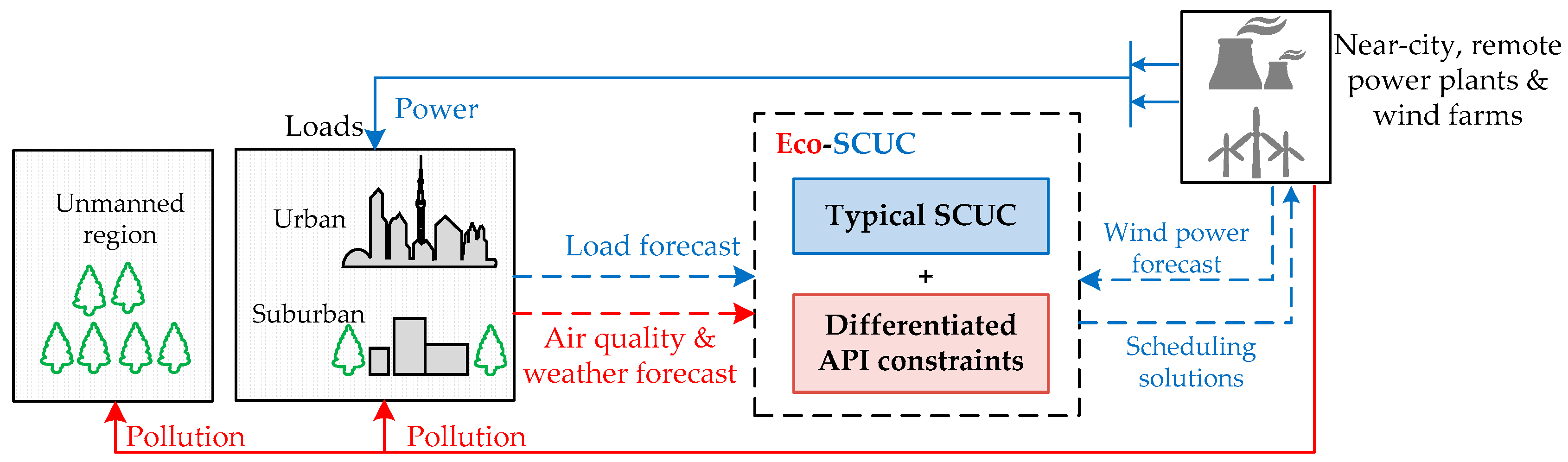
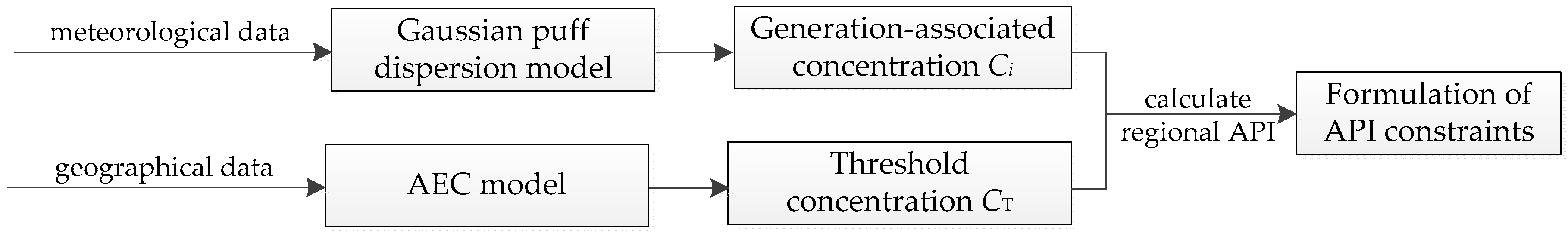
• Gaussian puff dispersion is used to model the transport of emissions, and the contribution of emissions to air pollutant concentration increments in targeted regions is calculated. The API is calculated as the ratio of local air pollutant concentration to local AEC-based threshold concentration. The API constraints are formulated and integrated into typical SCUC.
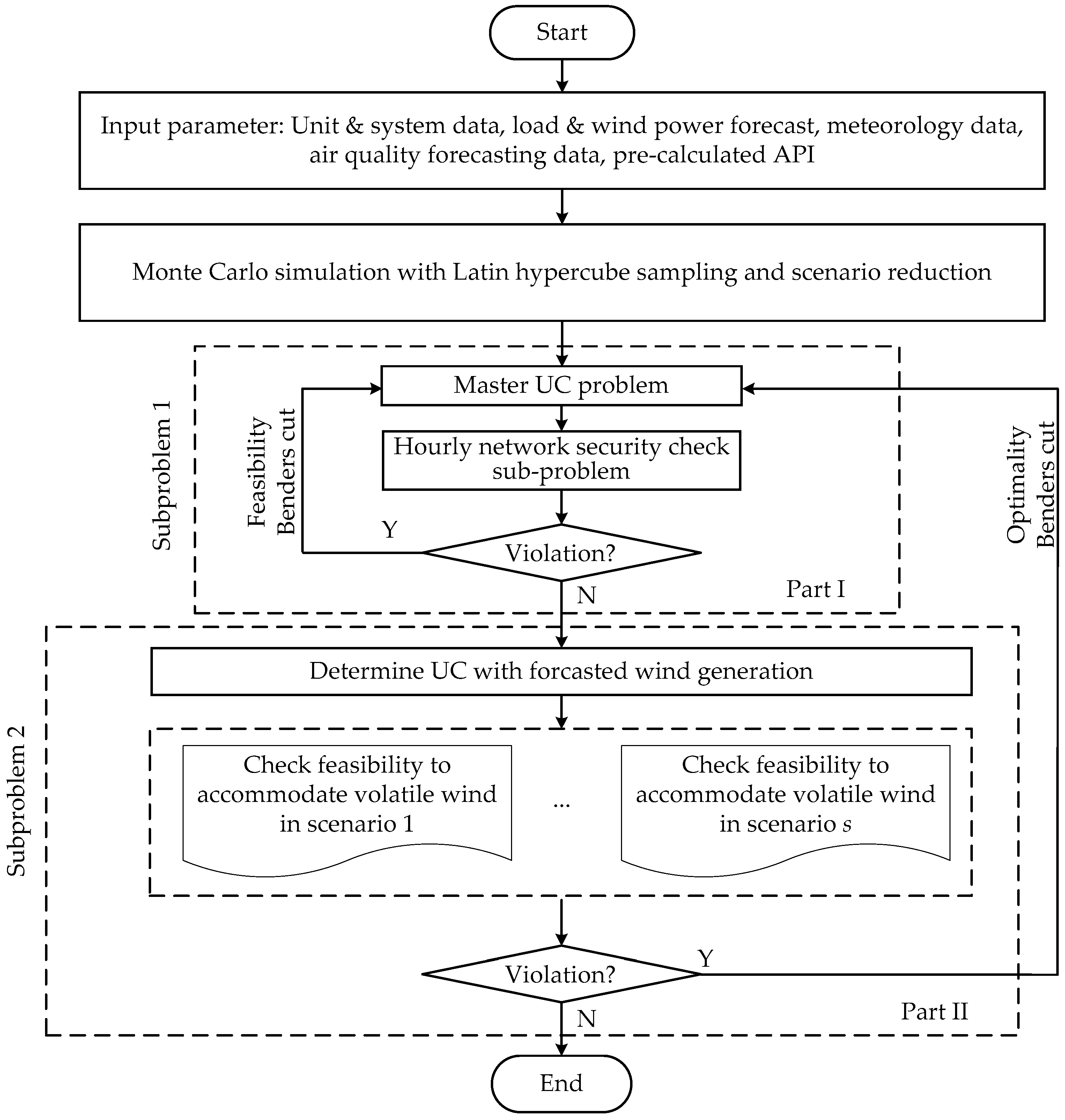
• The Monte Carlo simulation with Latin hypercube sampling (LHS) and scenario reduction is used to generate wind power volatility scenarios. Additionally, Benders decomposition is used to solve the formulated stochastic mixed-integer quadratic programming (MIQP) problem.
• Case studies prove the effectiveness of the proposed model in improving air quality for densely populated region and reducing the person-hours exposed to severe air pollution for the entire region via shifting generation among units.
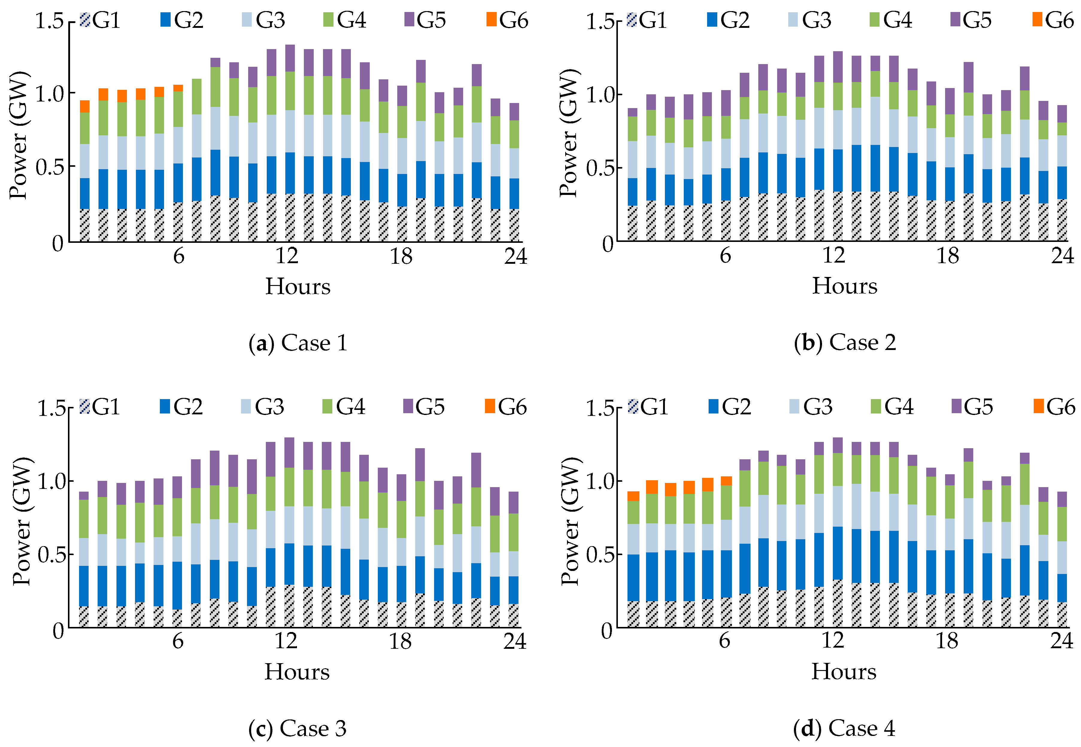
• Compared to undifferentiated dispatches, the Eco-SCUC considers trans-regional pollutant dispersion effects and differentiated population exposure to harmful pollutants. Instead of enforcing uniform regulations on emission, API constraints are formulated according to the differentiated impacts of coal-fired units on regional air quality. The model succeeds in mitigating the air pollution in densely-populated regions via shifting generation away from high-impact units to low-impact units and wind power.

The environmental benefits that the Eco-SCUC model can deliver are as follows: firstly, it can balance air pollution between densely-populated regions and sparsely-populated regions, thereby alleviating urban air pollution pressure; secondly, as the model schedules generation with respect to the differentiated impacts of units on regional air quality, it can reduce the average and peak concentrations of air pollutant in populated regions and help improve the level of air quality assessment of the city; thirdly, it significantly reduces the person-hours exposed to harmful air pollutants, such as SO₂, and abates the associated human health impacts. Note that the proposed model does not include chemical conversion from primary pollutants to secondary pollutants for now, and integrating secondary pollutants into the Eco-SCUC model requires greater research effort.

The rest of this paper is organized as follows: Section 2 formulates the differentiated API constraints; Section 3 describes the wind power generation scenarios; Section 4 formulates the Eco-SCUC and provides the solution methodology; and Section 5 presents the case studies while the conclusion is drawn in Section 6.

2. Formulating Differentiated API Constraints

In order to formulate regional differentiated API constraints, two critical parameters need to be ascertained using applicable methods: generation-associated concentration and regional threshold concentration. The former generally refers to the contribution of emissions of power plants to the pollutant concentration at predefined location. Therefore, it is necessary to include a deterministic and accurate dispersion model which can accommodate the varying meteorological conditions. In this context, a Gaussian puff dispersion model is applied to capture the dynamic transport of air pollutants from the emitting units to the concentration monitoring point. Secondly, the threshold concentration at the predefined location reflects the air pollutant carrying capacity in the concerned region, which depends on its AEC, population, area, etc. In this paper, an AEC method is employed to determine the threshold concentration of air pollutants with respect to geographical variations. The methodology of API constraints formulation is shown in Figure 2, and the modeling of the Gaussian puff model and AEC model is presented in the following sub-sections accordingly.

2.1. Gaussian Puff Dispersion

There are two commonly used air dispersion models: the steady-state Gaussian plume model and the integrated Gaussian puff model. The former is based on the assumption of constant wind speed and unchanging wind directions [34]. In comparison, the latter can accommodate fluctuating wind directions, wind speeds, and atmospheric stabilities [30]. Thus, the Gaussian puff model is used to describe the link between emissions at stacks (source) and air pollutant concentrations in polluted regions (receptor). The diagram of the Gaussian puff model is shown in Figure 3.

The Gaussian puff dispersion function is expressed as follows [34]:

$$G_i(\tau ,t;x,y,z)=\frac{1}{{(2\pi )}^{3/2}{\sigma }_x(\tau ,t){\sigma }_y(\tau ,t){\sigma }_z(\tau ,t)e^{\Psi /2}}$$

(1)

The intermediary parameter Ψ is calculated using Equations (A1) and (A2). When the atmospheric condition is steady, standard deviation σ_x/y/z(·) is in log-linear relation with respect to dispersion period (t – τ), which is expressed in (A3); when atmospheric condition is unsteady, the relationship is expressed in Equation (A4). The atmospheric stability class ϖ can be estimated by Pasquill grading method based on cloud coverage, solar radiation, wind speed and actual measurements [44]. The solar radiation level (−2 to +3) with respect to cloud coverage and solar altitude is given in

Table A1. Solar radiation classification according to total/low cloud coverage and solar altitude.

Total/Low Cloud Coverage (1/10)	Solar Altitude (°)
	Night	≤15	15–35	35–65	>65
≤4/≤4	−2	−1	+1	+2	+3
5–7/≤4	−1	0	+1	+2	+3
≥8/≤4	−1	0	0	+1	+1
≥5/5–7	0	0	0	0	+1
≥8/≥8	0	0	0	0	+1

; stability class ϖ (A–F) with respect to wind speed and solar radiation is given in

Table A2. Atmospheric stability classification according to wind speed and solar radiation level.

Ground-Level Wind Speed(m/s)	Solar Radiation Level
	+3	+2	+1	0	−1	−2
≤1.9	A	A–B	B	D	E	F
2–2.9	A–B	B	C	D	E	F
3–4.9	B	B–C	C	D	D	E
5–5.9	C	C–D	D	D	D	D
≥6	C	D	D	D	D	D

; relation between standard deviation and dispersion period with respect to ϖ is shown in Figure A1.

Based on Equation (1), the contribution of emissions to regional air pollutant concentration C_i is:

$$C_i(t;j)={\displaystyle \sum _{\tau }^{t-\tau }{Q}_i(\tau )G_i(\tau ,t;j)}$$

(2)

$$Q_i(t)=s_i{F}_i(p_{it})$$

(3)

$$F_i(p_{it})=(a_i{p}_{it}^2+b_i{p}_{it}+c_i)\Delta T$$

(4)

where j represents the location (x_j,y_j) in the targeted polluted region, in this paper we only care the ground-level concentration (assuming z ≈ 0).

2.2. Atmoshperic Environmental Capacity (AEC)

AEC represents the atmospheric stress limit within which the environmental system can return to its original condition [43]. Widely applied approaches to estimating AEC are: (1) A-value method; and (2) multisource modeling [45]. The latter requires accurate air quality model, such as the community multi-scale air quality (CMAQ) modeling. Its disadvantage is the neglect of accumulation-removal process of pollutants in the entire region. Thus, A-value method is applied in this paper. According to [43], for a given volume in atmosphere and time interval, AEC is defined as the removal rate of pollutant at the threshold concentration where the air pollutant emission rate (source) and removal rate (sink) reach the source-sink equilibrium. In the equilibrium, regional threshold concentration can be ascertained according to local AEC. The equilibrium is expressed in Equations (A5) and (A6), and the derived concentration and A-value is expressed in Equations (A7) and (A8).

When the generation and removal of air pollutant reach the equilibrium at location j and time t ($\overline{c}=C_{\mathrm{T},tj}, t\to \infty$), the threshold concentration at location j and time t can be expressed as:

$$C_{\mathrm{T},tj}=\frac{{\eta }_{tj}}{A_{tj}\sqrt{S_j}}$$

(5)

To sum up, the steps of calculating regional threshold concentration is as follows:

Step 1: Determine the removal rate of air pollutant η_tj.

The removal rate of air pollutant can be obtained via official environmental statistic Yearbooks or Bulletins. In this paper, climate-average values of AEC during the air pollution-prone seasons (November-February) are used, referring to [41].

Step 2: Determine A-value A_tj and examined area S_j.

A_tj can be calculated using Equation (A8), where U, H, v_d, and v_w are obtained through observation data or modeling data. This paper mainly concerns atmospheric ventilation and considers $A_{tj}=\sqrt{\pi }{U}_{tj}H/2$, where U_tj is hourly predicted wind speed and H = 276.85 m referring to winter-average H value in [41]. The resolution of S_j should be in consistency with that of η_tj and A_tj.

Step 3: Calculate the threshold concentration C_T,tj.

Based on the obtained η_tj, A_tj and S_j, regional C_T,tj are calculated by Equation (5).

2.3. Air Pollutant Intensity (API)

API is defined as the ratio of local air pollutant concentration to local threshold concentration:

$$AP{I}_i(t;j)=\frac{C_i(t;j)}{C_{\mathrm{T},tj}}\times 100\%$$

(6)

$$AP{I}_{0,tj}=\frac{C_{0,tj}}{C_{\mathrm{T},tj}}\times 100\%$$

(7)

$$API(t;j)={\displaystyle \sum _{i=1}^{NG}AP{I}_i(t;j)}+AP{I}_{0,tj}$$

(8)

where API_i(t;j) is calculated by Equations (2) and (6); API_0,tj is calculated by Equation (7); C_0,tj comes from 24-h air quality forecast from ground stations; C_T,tj is calculated by Equation (5). According to Equation (8), the API at the predefined location is the sum of all generation-associated APIs and background API.

Figure 4 shows the distribution of threshold concentration of SO₂ and API of SO₂ of one city in Northeast China, respectively. It illustrates that densely populated regions (low-AEC regions) have lower threshold concentrations and higher APIs.

2.4. Differentiated API Constraints

The differentiated API constraints can be expressed as:

$$API(t;j)\le \max \left\{AP{I}_{\mathrm{E},tj}, AP{I}_{0,tj}\right\} \forall j$$

(9)

API_E,tj refers to the expected API value at location j and time t, which is normally set to 100% (air pollutant saturated state). Additionally, the value of API_E,tj can be differentiated according to the local pollution level. For example, it can be set to higher value (>100%) when the air quality control is loosened in the targeted region; reversely, it can be set to lower value (<100%) when the region suffers severe air pollution and the air quality control is tightened.

When the background API value API_0,tj ≥ API_E,tj, the impacting units are expected to shut down or curtail their generation without violating system security constraints; when API_0,tj < API_E,tj, the impacting units are allowed to generate more to meet the load.

3. Formulating Wind Power Scenarios

The volatile and intermittent nature of wind leads to the inaccuracy of wind power prediction, challenging the secure operation of power system. According to [47], the intermittency refers to the unavailability of wind power within a relatively long period (≥1 h) and can be addressed by hourly wind forecast; the volatility refers to small fluctuations and can be mitigated by simulating possible wind power scenarios (<1 h). In this paper, the Weibull distribution is used to simulate the wind speed patterns [15], based on which the Monte Carlo simulation is used with LHS and scenario reduction techniques to generate possible wind power scenarios.

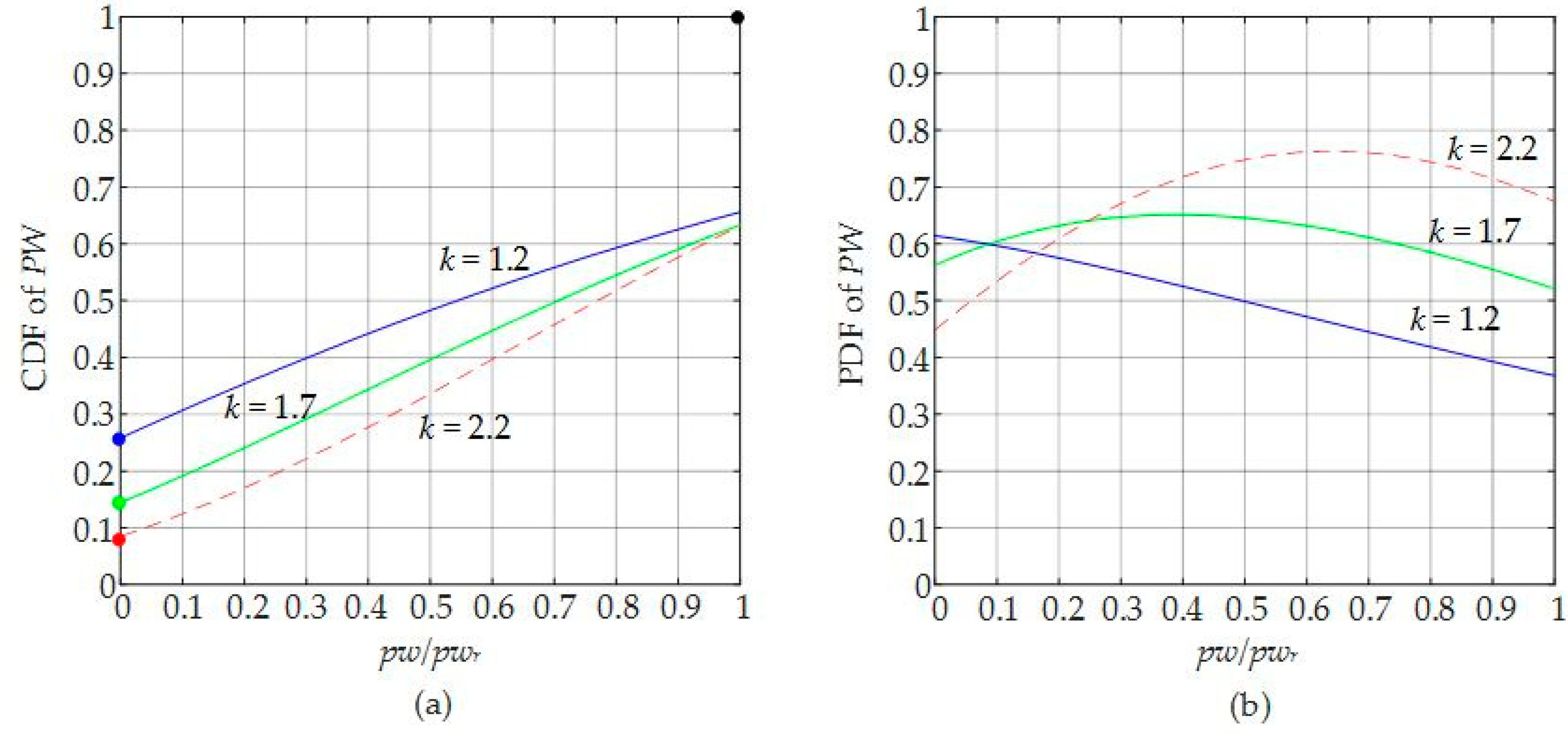
3.1. Distribution of Wind Speed

Field data suggest that wind speed at a given location follows Weibull distribution [48], whose cumulative distribution function (CDF) and probability density function (PDF) are:

$$F_V(v)={\displaystyle \underset{0}{\overset{v}{\int }}{f}_v(\lambda )d\lambda =}1-\exp \left[-{\left(\frac{v}{c}\right)}^k\right]$$

(10)

$$f_V(v)=\frac{k{v}^{k-1}}{c^k}\exp \left[-{\left(\frac{v}{c}\right)}^k\right], v\ge 0$$

(11)

The mean and standard variance of Weibull function is expressed by Equations (A9)–(A11). When k = 1, the distribution of V follows exponential distribution; when k = 2, the distribution of V follows Rayleigh distribution. To embrace the variety of wind speed patterns, our derivation of wind power distribution is based the general assumption that k > 0. Actual wind measurement data are used to estimate parameters c and k, as in Equations (A12) and (A13), and the estimation values are as in Equations (A14)–(A16).

3.2. Distribution of Wind Power

The relationship between wind power and wind speed depends on factors including generator efficiencies, wind rotor, inverter, gearbox and other wind turbine characteristics [49]. As shown in Figure A2, the simplified piecewise relationship can be expressed using Equation (A17). Two discrete probabilities for PW = 0 and PW = pw_r [50] are expressed in Equations (A18) and (A19). According to the theory for the function of random variables [15], the PDF and CDF of wind power can be expressed as:

$$f_{PW}(pw)=\frac{kh{v}_{\mathrm{in}}}{p{w}_{r}c}{\left[(1+\frac{hpw}{p{w}_r})v_{\mathrm{in}}/c\right]}^{k-1}\exp \left\{-{\left[(1+\frac{hpw}{p{w}_r})v_{\mathrm{in}}/c\right]}^k\right\}$$

(12)

$$F_{PW}(pw)=\mathrm{Pr}(PW\le pw)=\{\begin{array}{ll}0\hfill & (pw<0)\hfill \\ 1-\exp \left\{-{\left[(1+\frac{hpw}{p{w}_r})v_{\mathrm{in}}/c\right]}^k\right\}+\exp \left[-{\left(\frac{v_{\mathrm{out}}}{c}\right)}^k\right]\hfill & (0\le pw<p{w}_r)\hfill \\ 1\hfill & (pw\ge p{w}_r)\hfill \end{array}$$

(13)

$$h=\frac{v_r}{v_{\mathrm{in}}}-1$$

(14)

Examples of the CDF and PDF of wind power are plotted in Figure 5, respectively.

3.3. Scenario Generation and Reduction

To capture the stochastic availability of wind power, first, the Monte Carlo simulation is used to generate a large number of scenarios based on the wind power distribution and forecasted wind power. Second, LHS [47], which can be easily included in the Monte Carlo method, is applied to reduce the number of runs and achieve more appropriate random distribution of wind power. Simulation tests show that the Monte Carlo method with LHS can better approximate the required PDF of wind power than the simple Monte Carlo. Third, scenario reduction technique [51] is used to remain representing scenarios by eliminating scenarios of low probabilities and aggregating scenarios of close probabilities within an acceptable level of variation of the simulation precision.

4. Modeling Eco-SCUC

As shown in Figure 6, the proposed Eco-SCUC integrates differentiated API constraints into typical SCUC model for a hybrid power system consisting of coal-fired units and wind power generation. To accommodate wind power uncertainty, the day-ahead forecasted wind power and system load profile are required as electrical inputs for the Eco-SCUC. To differentiate the impacts of coal-fired units on regional air quality stress, the environmental inputs including air quality and weather forecasts are needed. The goal of the Eco-SCUC is to balance regional air quality stress among urban, suburban, and unmanned regions via shifting generation among units.

In this paper, SO₂ is assumed to be the major air pollutant in the targeted region, thus, it is taken as the single pollutant under study. However, the model can be extended to accommodate other single or multiple pollutants (e.g., NO_x, PM_2.5). This study does not consider chemical conversions from primary pollutants to secondary pollutants for now.

4.1. Integrating Wind Power Scenarios

SCUC with volatile wind power is formulated as a stochastic optimization [52] problem with the objective function of Equation (15) and constraints (Equations (16)–(36)). To consider the uncertainties of wind power, Monte Carlo simulation with LHS and scenario reduction techniques are used to generate possible scenarios based on the wind power distribution described in Equation (12). In each scenario, the simulated hourly random wind power will replace the forecasted hourly wind power in re-dispatch, thus, the hourly constraints (Equations (16)–(27)) are re-used as the scenario constraints (Equations (28)–(36)).

4.1.1. Objective Function

The objective function of typical SCUC is the sum of fuel, startup and shutdown costs of coal units, while assuming that the operating cost of wind-powered units is zero:

$$\min {\displaystyle \sum _{t=1}^{NT}{\displaystyle \sum _{i=1}^{NG}[{\gamma }_i{F}_i(p_{it})I_{it}+U_{it}}+D_{it}]}$$

(15)

where F_i(p_it) is calculated using Equation (4); and U_it/D_it is normally regarded as step function with respect to time t—in this paper we take it as a constant value for simplification.

4.1.2. Hourly Constraints

Hourly SCUC constraints include system power balance constraints (Equation (16)), wind power limit (Equation (17)), unit minimum on/off limits (Equations (18) and (19)), unit ramping up/down limits (Equations (20) and (21)), unit generation limits (Equation (22)), system regulation up/down limits (Equations (23) and (24)), system spinning/operating reserve limits (Equations (25) and(26)), and generalized DC power flow constraints (Equation (27)):

$${\displaystyle \sum _{i=1}^{NG}{p}_{it}{I}_{it}}+{\displaystyle \sum _{i=1}^{NW}p{w}_{it}}=P{D}_t+P{L}_t \forall t$$

(16)

$$0\le p{w}_{it}\le p{w}_{it}^f \forall i,\forall t$$

(17)

$$[X_{i,t-1}^{\mathrm{on}}-T_i^{\mathrm{on}}][I_{i,t-1}-I_{it}]\ge 0 \forall i,\forall t$$

(18)

$$[X_{i,t-1}^{\mathrm{off}}-T_i^{\mathrm{off}}][I_{i,t-1}-I_{it}]\ge 0 \forall i,\forall t$$

(19)

$$p_{it}-p_{i,t-1}\le [1-I_{it}(1-I_{i,t-1})]P_i^{\mathrm{RU}}+I_{it}(1-I_{i,t-1})P_{i.\min }$$

(20)

$$p_{i,t-1}-p_{it}\le [1-I_{i,t-1}(1-I_{it})]P_i^{\mathrm{RD}}+I_{i,t-1}(1-I_{it})P_{i.\min }$$

(21)

$$P_{i,\min }{I}_{it}\le p_{it}\le P_{i,\max }{I}_{it} \forall i,\forall t$$

(22)

$${\displaystyle \sum _{i=1}^{NG}R{U}_{it}{I}_{it}}\ge R{U}_t \forall t$$

(23)

$${\displaystyle \sum _{i=1}^{NG}R{D}_{it}{I}_{it}}\ge R{D}_t \forall t$$

(24)

$${\displaystyle \sum _{i=1}^{NG}R{S}_{it}{I}_{it}}\ge R{S}_t \forall t$$

(25)

$${\displaystyle \sum _{i=1}^{NG}R{O}_{it}{I}_{it}}\ge R{O}_t \forall t$$

(26)

$$\left|\mathit{S}\mathit{F}({\mathit{K}}_{\mathrm{P}}\mathit{P}+{\mathit{K}}_{\mathrm{W}}\mathit{P}\mathit{W}-{\mathit{K}}_{\mathrm{D}}\mathit{P}\mathit{D})\right|\le \mathit{P}\mathit{L}$$

(27)

4.1.3. Scenario Constraints

For each simulated scenario, the scenario constraints include system power balance constraints (Equation (28)), wind power limit (Equation (29)), unit generation limits (Equation (30)), system regulation up/down limits (Equations (31) and (32)), system spinning/operating reserve requirements (Equations (33) and (34)), generalized DC power flow constraints (Equation (35)) and permissible adjustment of real power generation limits (Equation (36)):

$${\displaystyle \sum _{i=1}^{NG}{p}_{it}^s{I}_{it}}+{\displaystyle \sum _{i=1}^{NW}p{w}_{it}^s}=P{D}_t+P{L}_t \forall t,\forall s$$

(28)

$$0\le p{w}_{it}^s\le p{w}_{it}^{f,s} \forall i,\forall t$$

(29)

$$P_{i,\min }{I}_{it}\le p_{it}^s\le P_{i,\max }{I}_{it} \forall i,\forall t,\forall s$$

(30)

$${\displaystyle \sum _{i=1}^{NG}R{U}_{it}^s{I}_{it}}\ge R{U}_t \forall t,\forall s$$

(31)

$${\displaystyle \sum _{i=1}^{NG}R{D}_{it}^s{I}_{it}}\ge R{D}_t \forall t,\forall s$$

(32)

$${\displaystyle \sum _{i=1}^{NG}R{S}_{it}^s{I}_{it}}\ge R{S}_t \forall t,\forall s$$

(33)

$${\displaystyle \sum _{i=1}^{NG}R{O}_{it}^s{I}_{it}}\ge R{O}_t \forall t,\forall s$$

(34)

$$\left|\mathit{S}\mathit{F}({\mathit{K}}_{\mathrm{P}}{\mathit{P}}^s+{\mathit{K}}_{\mathrm{W}}\mathit{P}{\mathit{W}}^s-{\mathit{K}}_{\mathrm{D}}\mathit{P}\mathit{D})\right|\le \mathit{P}\mathit{L} \forall s$$

(35)

$$\left|p_{it}^s-p_{it}\right|\le {\Delta }_i \forall i,\forall t,\forall s$$

(36)

Equation (36) ensures that the re-dispatch of coal-fired units can accommodate the volatility of wind power. For each scenario and time interval, Equation (36) is applied for mitigating the violations based on which corrective and preventive actions are formulated. Δ_i represents the adjustable magnitude of real power of coal-fired units in ten minutes (i.e., 10/60 of hourly ramping rate of units) [47].

4.2. Integrating API Constraints

The differentiated API constraints are expressed in Equation (9). As the violation of API constraints may fail the optimal solution to the formulated MIQP problem, the big M-slack method is employed. The objective function of the proposed model can be expressed as:

$${\displaystyle \sum _{t=1}^{NT}{\displaystyle \sum _{i=1}^{NG}[{\gamma }_i{F}_i(p_{it})I_{it}+U_{it}}+D_{it}]}+{\displaystyle \sum _{t=1}^{NT}{\displaystyle \sum _{j=1}^{NJ}{M}_{tj}\cdot \max \left\{{\zeta }_{tj},0\right\}}}$$

(37)

$$API(t;j)-\max \left\{AP{I}_{\mathrm{E},tj},AP{I}_{0,tj}\right\}={\zeta }_{tj}$$

(38)

where M_tj is the penalty function determined by different environmental-justice-associated factors, such as geographical population, regional GDP, ecological GDP, etc., in this paper, M_tj is taken as a large enough constant for simplicity; ζ_tj is the artificial slack variable which is calculated using Equation (38).

The objective function of the Eco-SCUC is the minimization of total cost including the penalties caused by violation of regional API constraints as expressed in Equation (37), and the constraints include hourly SCUC constraints (Equations (16)–(27)) and wind power scenario constraints (Equations (28)–(36)). The Eco-SCUC incorporating API constraints and volatile wind power can be expressed as:

min (37)

s.t. (16)–(36), (38)

4.3. Solution Methodology

To reduce the computation burden of the formulated MIQP, Benders decomposition technique is applied to unbundle the problem into a master UC problem followed by a network security check sub-problem. Furthermore, re-dispatch will be conducted for accommodating the volatility of wind power in the scenario feasibility check sub-problems. If any violation appears in the sub-problems, the Benders cuts will be created and added to master UC problem. The flowchart of the two-stage algorithm is plotted in Figure 7.

Step 1: the input parameters including unit data, system data, 24-h load forecast, hourly wind power forecast, predicted meteorological conditions, regional background API data are collected;

Step 2: Monte Carlo simulation with LHS is applied to generate hourly wind power volatility scenarios; the number of possible scenarios is reduced by scenario reduction technique;

Step 3: the initial dispatch is checked in the hourly network security check sub-problem 1 in the first stage (part I); if any violation occurs, feasibility Benders cut will constrain the violating unit outputs and will be added to the master UC problem for updating new commitment;

Step 4: the re-dispatch for accommodating wind power volatility is considered in the scenario feasibility check sub-problem 2 in the second stage (part II); if any violation occurs, optimality Benders cut will prevent and revise the commitment solution and will be added to the master UC problem; the scenario check sub-problem is optimized by Equation (36); and

Step 5: the iterations between the master UC problem and feasibility check sub-problem will continue until the generation re-dispatch can satisfy the simulated wind power scenarios.

Detailed descriptions about Benders decomposition can be referred to [13,47]. The formulated MIQP can be solved by multiple commercial solvers [53]. In this paper, the problem is solved using CPLEX 12.1 optimizer in MATLAB (MathWorks, Natick, MA, USA).

5. Case Studies

5.1. Description

The Eco-SCUC is tested for a 24-h period in a 14-bus power system consisting of six6 coal units and wind power. Figure 8 shows the geographical distribution of the units (G1–G6) and regions (R1–R5) with differentiated threshold concentrations. The wind turbines are integrated at Bus 9.

Parameters of system are listed as follows:

Table A3. Fuel consumption coefficients and stack parameters of coal-fired units.

Unit	Fuel Consumption Coefficients				Stack Parameters
	ai (ton/MW2h)	bi (ton/MWh)	ci (ton/h)	si (ton/ton)	xs (km)	ys (km)	zs (m)
G1	0.001076	0.050572	21.2	0.00487	3	14	150
G2	0.000960	0.050052	24.8	0.00465	23	9	150
G3	0.001052	0.056072	16.0	0.00455	7	2	135
G4	0.001132	0.063940	16.8	0.00495	22	24	105
G5	0.001176	0.068860	13.2	0.00425	15	5	135
G6	0.001528	0.069864	12.4	0.00413	8	18	135

lists the fuel consumption coefficients and stack parameters of coal units;

Table A4. Generation costs, on/off limits, generation limits, and ramping limits of units.

Unit	Generation Costs			On/Off Limits		Generation Limits		Ramp Limits
	γi ($/ton)	Uit ($)	Dit ($)	Ton (h)	Toff (h)	Pi,min (MW)	Pi,max (MW)	${\mathit{P}}_{\mathit{i}}^{\mathbf{R}\mathbf{U}}$/${\mathit{P}}_{\mathit{i}}^{\mathbf{R}\mathbf{D}}$ (MW)
G1	55.572	623.6	374.1	5	5	360	80	120/120
G2	55.884	501.2	213.0	5	5	380	100	125/125
G3	60.360	497.6	186.6	4	4	290	75	80/80
G4	60.624	428.7	264.3	4	4	280	110	115/115
G5	60.836	423.5	236.7	3	3	295	120	120/120
G6	63.712	202.5	113.6	2	2	120	25	60/60

shows the generation costs, on/off limits, generation limits, ramping limits of coal units; and

Table A5. Transmission line impedances and power flow limits.

Line	Initial Bus	Terminal Bus	Impedance (p.u.)	Power Flow Limit (MW)
1	1	2	0.170	250
2	1	5	0.258	180
3	2	3	0.150	175
4	2	4	0.197	185
5	2	5	0.140	225
6	3	4	0.018	320
7	4	5	0.037	175
8	4	7	0.037	195
9	4	9	0.150	200
10	5	6	0.187	225
11	6	11	0.197	450
12	6	12	0.197	150
13	6	13	0.150	180
14	7	8	0.140	380
15	7	9	0.019	260
16	9	10	0.039	325
17	9	14	0.037	255
18	10	11	0.152	250
19	12	13	0.183	150
20	13	14	0.192	260

lists the transmission line impedances and power flow limits. The population in R1–R5 is 2.65, 1.13, 0.56, 0.27, and 0.08 million, respectively.

Forecasted parameters are listed as follows:

Table A6. Hourly forecasted wind power and system load.

t	$\mathit{p}{\mathit{w}}_{\mathit{i}\mathit{t}}^{\mathit{f}}$ (MW)	Bus-Load (MW)
		Bus 4	Bus 5	Bus 7	Bus 9	Bus 10	Bus 11	Bus 12	Bus 13
1	142. 6	190.2	113.1	83.7	98.4	93.8	177.1	107.1	55.2
2	131.0	204.2	121.4	89.9	105.6	100.8	190.1	115.0	59.1
3	123.8	203.6	121.1	89.6	105.3	100.5	189.5	114.7	58.8
4	142. 6	205.4	122.1	90.4	106.2	101.3	191.2	115.7	59.4
5	123.8	207.4	123.3	91.3	107.3	102.3	193.1	116.8	59.9
6	105.1	212.1	126.1	93.3	119.7	104.7	197.5	119.5	61.3
7	96.5	237.2	141.0	104.4	122.7	117.0	220.8	133.6	68.5
8	89.3	252.0	149.8	110.9	130.3	124.3	215.9	151.9	82.8
9	110.9	236.0	146.3	108.2	127.3	121.4	225.3	138.6	71.1
10	112.3	234.0	135.0	99.9	117.5	111.4	227.8	137.4	70.5
11	128.2	267.7	145.1	122.2	133.6	137.0	221.3	156.4	73.8
12	148.3	254.7	149.2	125.2	137.2	140.5	247.1	160.3	69.4
13	207.4	263.0	148.2	124.5	126.4	139.6	235.5	154.1	72.6
14	198.7	260.8	136.9	123.5	135.2	138.5	234.2	158.1	74.7
15	193.0	263.6	128.6	124.8	136.7	139.9	236.1	154.4	66.4
16	185.7	249.7	118.4	109.9	129.2	123.2	223.1	140.6	72.1
17	184.3	225.6	114.1	99.3	116.7	121.3	220.0	127.1	65.2
18	174.2	214.1	127.3	94.2	129.7	105.6	199.3	120.6	61.9
19	63.5	246.2	136.4	108.3	127.3	121.5	229.2	165.8	85.1
20	86.5	206.0	122.4	90.6	106.5	101.6	191.7	116.0	59.5
21	110.9	211.1	125.5	92.9	109.2	104.2	196.5	118.9	61.0
22	119.5	245.7	146.0	108.1	127.1	121.2	228.7	138.4	71.0
23	138.2	197.4	117.4	86.9	102.1	97.4	183.8	111.2	57.0
24	146.9	191.7	114.0	84.4	99.2	94.6	181.3	108.1	55.4

gives the hourly forecasted wind power and system load;

Table A7. Hourly simulated and reduced wind power volatility scenarios.

t	Wind Power Volatility Scenario (MW)
	1	2	3	4	5	6	7	8	9	10
1	144.9	146.8	148.7	146.8	146.6	146.9	143.7	137.9	141.3	140.1
2	133.7	135.4	133.9	136.8	133.5	128.6	126.9	128.3	129.8	130.1
3	121.5	120.9	122.0	121.1	120.2	119.7	118.9	114.3	113.5	114.4
4	145.6	146.8	148.0	145.8	143.4	143.4	145.8	148.7	149.4	148.8
5	124.7	122.7	120.7	119.2	121.0	121.7	118.8	125.2	122.8	124.8
6	103.5	104.1	102.2	102.8	101.9	99.4	97.2	92.4	94.3	95.4
7	95.5	93.3	93.3	93.2	93.4	91.1	89.5	90.8	92.6	94.8
8	89.6	88.7	90.8	90.2	88.7	89.5	90.2	89.8	91.3	95.5
9	113.5	111.7	110.2	112.1	112.7	117.0	118.4	124.6	123.2	122.2
10	115.4	112.7	113.2	113.7	112.4	112.1	113.0	121.8	122.4	117.0
11	126.1	128.2	126.5	126.9	127.9	130.6	130.3	135.1	131.9	132.7
12	151.8	153.3	155.3	158.6	160.2	156.5	156.9	147.7	147.2	149.3
13	212.2	210.3	207.8	205.6	208.2	219.2	197.9	212.4	210.5	209.7
14	198.6	203.1	203.2	205.9	205.4	200.5	203.1	202.3	199.9	195.9
15	195.9	191.4	193.4	195.9	191.9	184.9	182.1	177.3	170.3	168.4
16	182.4	181.9	185.5	174.4	182.0	181.8	189.8	193.6	192.9	189.6
17	183.6	182.6	186.8	187.5	191.4	191.2	188.2	187.9	184.1	182.1
18	177.9	180.3	180.8	177.0	174.0	172.3	171.2	167.2	168.1	167.6
19	64.5	60.5	64.4	69.3	64.1	62.7	63.1	64.6	64.6	62.7
20	88.5	87.2	85.7	85.9	86.1	80.2	87.3	82.9	83.8	83.7
21	111.8	111.8	110.5	112.1	114.9	113.6	111.3	109.5	110.6	115.7
22	116.8	116.5	118.5	121.1	118.6	120.5	123.1	131.3	132.3	122.5
23	140.7	141.8	140.1	137.6	137.3	140.6	142.6	138.8	135.6	128.7
24	150.1	151.7	154.1	154.7	151.7	159.6	151.5	147.4	144.3	145.3

shows the simulated wind power scenarios (1–10) based on a standard deviation of 10% of the predicted wind power as listed in Table A6;

Table A8. Hourly forecasted wind speed, wind direction, and atmospheric stability near units.

t	G1			G2			G3			G4			G5			G6
	v1	φ1	ϖ1	v	φ	ϖ	v	φ	ϖ	v	φ	ϖ	v	φ	ϖ	v	φ	ϖ
1	7.6	292	D	15.2	290	E	3.2	310	E	13.1	290	D	13.2	20	E	8.6	337	F
2	8.3	285	D	15.4	295	E	4.3	333	E	13.4	284	D	14.2	18	E	8.4	343	F
3	7.8	281	D	15.0	301	E	4.3	323	E	12.9	280	D	13.5	15	E	8.5	349	F
4	6.9	275	D	14.2	304	E	4.6	320	E	12.4	283	D	13.7	7	E	7.9	356	F
5	6.4	276	D	14.9	310	E	4.2	317	E	12.1	286	D	13.0	9	E	7.5	348	F
6	6.2	271	D	14.0	312	E	5.3	304	E	11.5	291	D	12.2	4	E	6.5	355	F
7	5.3	270	F	14.1	318	F	5.6	302	D	10.5	283	F	11.0	354	F	5.5	357	D
8	5.0	270	F	14.1	317	F	4.9	305	D	10.4	276	F	11.0	350	F	5.3	355	D
9	5.1	274	F	14.3	316	F	6.3	311	D	10.2	273	F	11.2	359	F	5	355	D
10	5.2	277	F	14.5	315	F	5.3	313	D	10.7	269	F	11.3	2	F	5.1	5	D
11	5.4	275	F	14.6	315	F	4.3	315	D	10.3	268	F	11.1	8	F	5.3	4	D
12	5.0	269	F	14.3	320	F	5.1	305	D	10.2	271	F	11.5	355	F	5.4	358	D
13	5.3	268	F	14.2	310	E	6.3	298	F	10.2	270	C	11.6	357	E	5.9	3	F
14	5.3	270	F	14.2	319	E	6.4	295	F	10.3	275	C	10.8	354	E	5.7	356	F
15	4.9	274	F	14.5	316	E	7.3	290	F	10.4	276	C	10.9	7	E	5.1	2	F
16	5.1	275	F	14.3	315	E	6.3	285	F	10.1	273	C	10.8	3	E	5.2	3	F
17	5.0	272	F	14.3	315	E	5.3	294	F	10.1	275	C	11.1	355	E	5	355	F
18	5.5	274	F	14.1	319	D	4.2	303	E	10.2	276	C	11.0	355	D	5.2	360	D
19	5.5	279	F	15.5	310	D	6.3	300	E	12.4	273	C	11.8	358	D	5.6	355	D
20	6.1	281	F	15.9	308	D	5.9	322	E	12.6	276	C	11.9	360	D	6.3	352	D
21	6.4	284	F	16.5	304	D	5.5	318	E	11.9	284	C	12.5	360	D	6.5	356	D
22	7.4	295	F	17.5	310	D	5.9	323	E	11.0	297	C	13.4	345	D	7.0	354	D
23	7.9	292	D	17.9	296	D	6.0	325	E	12.6	292	C	14.5	339	D	7.5	331	D
24	8.0	296	D	16.5	292	D	6.3	316	E	12.9	302	C	14.6	331	D	7.2	345	D

¹ In this table, v represents the wind speed, in m/s; φ represents the wind direction, in °; and ϖ represents the Pasquill atmospheric stability class, in A–F.

provides the hourly forecasted wind speed, wind direction and atmospheric stability class near coal units; and

Table A9. Hourly forecasted regional background and threshold concentration of SO₂.

t	Background Concentration C0,tj (μg/m3)					Threshold Concentration CT,tj (μg/m3)					Background API API0.tj (%)
	R1 1	R2	R3	R4	R5	R1	R2	R3	R4	R5	R1	R2	R3	R4	R5
1	34.5	32.2	31.9	28.8	25.3	35.7	38.2	40.3	42.5	60.2	96.6	84.3	79.1	67.8	42.0
2	33.2	31.6	29.8	26.7	23.2	35.7	38.2	40.3	42.5	60.2	93.0	82.7	73.9	62.8	38.5
3	31.5	30.2	28.7	25.5	21.9	35.7	38.2	40.3	42.5	60.2	88.2	79.1	71.2	60.0	36.4
4	30.8	29.8	28.8	25.7	21.5	35.3	37.5	39.8	42.3	60.2	87.3	79.5	72.4	60.8	35.7
5	31.5	30.3	28.8	25.8	22.5	35.3	37.5	39.8	42.3	60.2	89.2	80.8	72.4	61.0	37.4
6	33.6	32.4	29.3	26.1	23.6	35.3	37.5	39.8	42.3	60.2	95.2	86.4	73.6	61.7	39.2
7	36.4	33.5	30.7	26.9	24.3	35.1	37.5	39.5	42.2	59.5	103.7	89.3	77.7	63.7	40.8
8	39.4	35.8	32.5	28.5	25.1	35.1	37.5	39.5	42.2	59.5	112.3	95.5	82.3	67.5	42.2
9	43.9	39.1	34.8	29.8	26.8	35.1	37.5	39.5	42.2	59.5	125.1	104.3	88.1	70.6	45.0
10	48.5	42.7	38.9	32.4	27.9	34.4	36.9	39.5	41.6	59.5	141.0	115.7	98.5	77.9	46.9
11	52.9	46.8	42.6	34.5	31.4	34.4	36.9	39.5	41.6	59.5	153.8	126.8	107.8	82.9	52.8
12	53.1	48.3	43.8	36.8	34.2	34.4	36.9	39.5	41.6	59.5	154.4	130.9	110.9	88.5	57.5
13	52.9	48.1	43.5	36.5	33.6	34.6	36.9	39.4	41.6	59.3	152.9	130.4	110.4	87.7	56.7
14	51.8	45.2	42.7	36.4	33.5	34.6	36.9	39.4	41.6	59.3	149.7	122.5	108.4	87.5	56.5
15	48.2	45.1	41.6	35.9	32.8	34.6	36.9	39.4	41.6	59.3	139.3	122.2	105.6	86.3	55.3
16	48.1	44.1	41.7	35.2	31.9	34.5	36.6	40.2	41.5	59.3	139.4	120.5	103.7	84.8	53.8
17	50.1	43.2	40.7	35.0	32.4	34.5	36.6	40.2	41.5	59.3	145.2	118.0	101.2	84.3	54.6
18	54.2	47.2	43.8	36.6	34.7	34.5	36.6	40.2	41.5	59.3	157.1	129.0	109.0	88.2	58.5
19	53.9	46.9	43.2	35.4	35.1	34.5	37.2	40.2	41.5	60.1	156.2	126.1	107.5	85.3	58.4
20	50.2	44.3	41.5	34.2	33.2	34.5	37.2	40.2	41.5	60.1	145.5	119.1	103.2	82.4	55.2
21	47.0	42.1	38.9	32.4	32.4	34.5	37.2	40.2	41.5	60.1	136.2	113.1	96.8	78.1	53.9
22	43.1	38.2	35.1	30.1	30.1	35.2	37.5	40.4	42.4	60.1	122.4	101.9	86.9	71.0	50.1
23	40.7	36.2	32.5	27.9	27.5	35.2	37.5	40.4	42.4	60.1	115.6	96.5	80.4	65.8	45.8
24	38.1	34.6	32.3	28.3	26.6	35.2	37.5	40.4	42.4	60.1	108.2	92.3	80.0	66.7	44.3

¹ In this table, R1–R5 represents the region 1–5 as shown in Figure 8.

lists the forecasted hourly background concentration, threshold concentration, and calculated regional background API of SO₂.

5.2. Results

Four cases are studied in this paper:

Case 1: typical SCUC minimizing the total costs, neither wind generation nor API constraints are included; Case 2: typical SCUC minimizing the total costs, considering wind generation, but the API constraints are still absent; Case 3: typical SCUC minimizing the total emissions, considering wind generation, but the API constraints are still absent; and Case 4: the Eco-SCUC, considering both wind generation and API constraints, the API expectation value is set to 100% (API_E,tj = 100%).

Comparisons are made among Cases 1–4. Figure 9 shows the generation results of G1-G6; Figure 10 compares their hourly total emissions; Figure 11 shows the geographical distribution of API increases (ΔAPI) at 6:00, 12:00, 18:00, and 24:00, respectively.

As shown in Figure 9, the hourly generation results of G1-G6 in Cases 1–4 are different. As Case 1 does not consider wind power, it has higher hourly generation compared to Cases 2–4. Cases 2 and 3 have different results because they schedule generation according to the minimization of the fuel cost and total emission, respectively. In comparison, the hourly generation of G3 and G5 in Case 4 (Eco-SCUC) is obviously lower. This is because, according to geographical locations (see Figure 8) and wind directions (see Table A8), G3 and G5 are situated upwind of densely-populated R1 and R2, thus, wind brings pollutants from the units downwind to densely-populated regions. Taking into account differentiated API constraints, Case 4 will curtail generation of G3 and G5 to reduce the resulting API increments in R1 and R2. Conversely, generation of other units is increased to meet the load.

As shown in Figure 10, Case 1 has the highest hourly total emission among the four cases during most times of the day, because it does not contain wind power. Generally, Case 3 has the lowest hourly emissions, because the objective of Case 3 is to minimize total emissions of system. Finally, Case 4 sometimes has higher hourly emissions because it schedules generation according to the differentiated impacts of units on regional air quality, instead of the merely low emission rate of the unit. In other words, the unit that has a low emission rate may have a high impact on the regional API.

As shown in Figure 11, Case 1 without wind power has the worst ΔAPI distribution results compared with Cases 2–4, for example, its ΔAPI in densely-populated R1 is the highest among the four cases. Compared to Cases 1–3, Case 4 (Eco-SCUC) has the lowest ΔAPI in densely-populated regions because, as stated above, Eco-SCUC schedules the generation of units according to their differentiated impacts on regional API. In order to justify the effectiveness of the Eco-SCUC in mitigating regional air pollution, comparisons on different cases, units, and regions are made in

Table 1. Comparisons of total cost, total fuel, total emission, and SO₂ concentrations at R1–R5.

Case	Cost (103$)	Fuel (ton)	Emission (ton)	Cav (μg/m3)					Cpk (μg/m3)
				R1	R2	R3	R4	R5	R1	R2	R3	R4	R5
1	595.93	10138.0	55.4	60.2	57.6	52.9	41.3	38.1	70.7	68.2	65.1	53.2	49.0
2	512.73	8683.8	50.5	59.9	55.7	50.4	40.1	36.5	68.8	63.9	57.3	48.4	45.4
3	523.46	8957.2	48.5	55.5	51.2	47.1	38.2	31.2	66.4	60.1	53.3	45.1	43.1
4	527.62	9174.2	53.2	50.2	47.0	43.3	35.3	39.8	57.9	54.3	48.4	41.4	49.6

,

Table 2. Comparisons of total generation and daily average generation-associated API in Cases 3 and 4.

Unit	Traditional SCUC (Case 3)						Eco-SCUC (Case 4)
	Generation (MW)	ΔAPIi,av 1					Generation (MW)	ΔAPIi,av 1
		R1	R2	R3	R4	R5		R1	R2	R3	R4	R5
G1	4763.7	0.0%	0.3%	0.0%	0.0%	0.7%	5572.5	0.0%	0.5%	0.0%	0.0%	3.4%
G2	5334.9	0.5%	0.0%	0.0%	5.6%	0.9%	6015.8	0.8%	0.0%	0.0%	6.8%	5.1%
G3	5518.5	1.1%	15.6%	12.3%	0.0%	1.1%	5044.2	0.8%	9.4%	9.1%	0.0%	0.9%
G4	4239.1	0.6%	0.2%	0.0%	0.4%	0.6%	4763.9	0.9%	0.3%	0.0%	0.6%	1.2%
G5	3678.4	31.4%	14.4%	13.5%	9.8%	0.5%	1622.1	15.9%	7.1%	7.2%	1.5%	0.4%
G6	0.0	0.0%	0.0%	0.0%	0.0%	0.0%	516.1	0.0%	0.0%	0.0%	0.0%	7.1%
Total	23534.6	33.6%	30.5%	25.8%	15.8%	3.8%	23534.6	18.4%	17.3%	16.3%	8.9%	18.1%

¹ ΔAPI_i,av represents daily average value of regional API increment caused by coal-fired unit.

and

Table 3. Comparisons of pollutant saturated hours and sum of person-hour exposed to pollutant saturation in an annual case.

Case	Ts (Hour)					P × Ts (109 Person·Hour)
	R1	R2	R3	R4	R5	Sum of R1–R5
1	1101	733	411	194	59	4.078
2	1056	685	398	181	55	3.754
3	1063	719	379	178	57	3.894
4	561	437	316	153	63	2.204

.

As shown in Table 1, Case 1 suffers the most total cost, total fuel, total emission, and regional SO₂ concentration compared to other cases, this is mainly because there are no wind power and API constraints in Case 1. Furthermore, comparisons among Cases 2–4 show that Case 4 suffers 2.9% more total cost than Case 2 and 9.7% more total emissions than Case 3. However, the resulting concentrations in Case 4 are much lower: in densely-populated R1, C_av reduces 16.2% from Case 2, and C_pk reduces 12.8% from Case 3. In sparsely populated regions, API constraints in the Eco-SCUC may lead to an increase of pollutant concentration, explaining that in Case 4, C_av and C_pk in R5 increase to 39.8 μg/m³ and 49.6 μg/m³, respectively. This proves that, via shifting generation among units, the Eco-SCUC can cost-effectively mitigate pollution in densely-populated regions while the concentrations in sparsely-populated regions do not exceed local threshold concentrations.

As shown in Table 2, the hourly generation of G1–G6 varies significantly between Case 3 and Case 4. Accordingly, the resulting regional ΔAPI is different (see Figure 11). It can be observed that Case 4 (Eco-SCUC) can effectively mitigate total ΔAPI for densely populated R1–R4 compared to Case 3, while ΔAPI in less densely populated R5 augments from 3.8% to 18.1%. However, C_av and C_pk in R5 in Case 4 are still below its threshold concentration. This phenomenon stems from the integration of differentiated API constraints in the Eco-SCUC. To be specific, G3 and G5 (underlined) are taken as high-impact units and their generation is curtailed, while generation of other units is augmented to meet the load. This justifies that via shifting generation away from high-impact units to low-impact ones, the Eco-SCUC can drive the potential air pollution away from densely-populated regions to sparsely populated ones.

To illustrate the effects in a larger scale, 48 historical samples of meteorological data are used to represent an annual case. Table 3 compares the annual pollutant saturated hours (T_s) in R1–R5 and the annual sum of person-hours (P × T_s) exposed to saturated pollutant for the whole region.

As shown in Table 3, T_s in R1 in Case 4 is nearly half of the value in Cases 1–3, which indicates that under the Eco-SCUC, densely populated regions face much less air pollution. In return, T_s in R5 in Case 4 is 4 h per year more than Case 1, which has little impact on sparsely populated R5. Once the system includes other regions with much lower population density, T_s in R1–R5 will all decrease. In the whole, the annual sum of person-hour in Case 4 in R1–R5 is 54.0% of that in Case 1, which proves that the Eco-SCUC can protect much more residents from severe air pollution.

From the above results, several conclusions can be drawn:

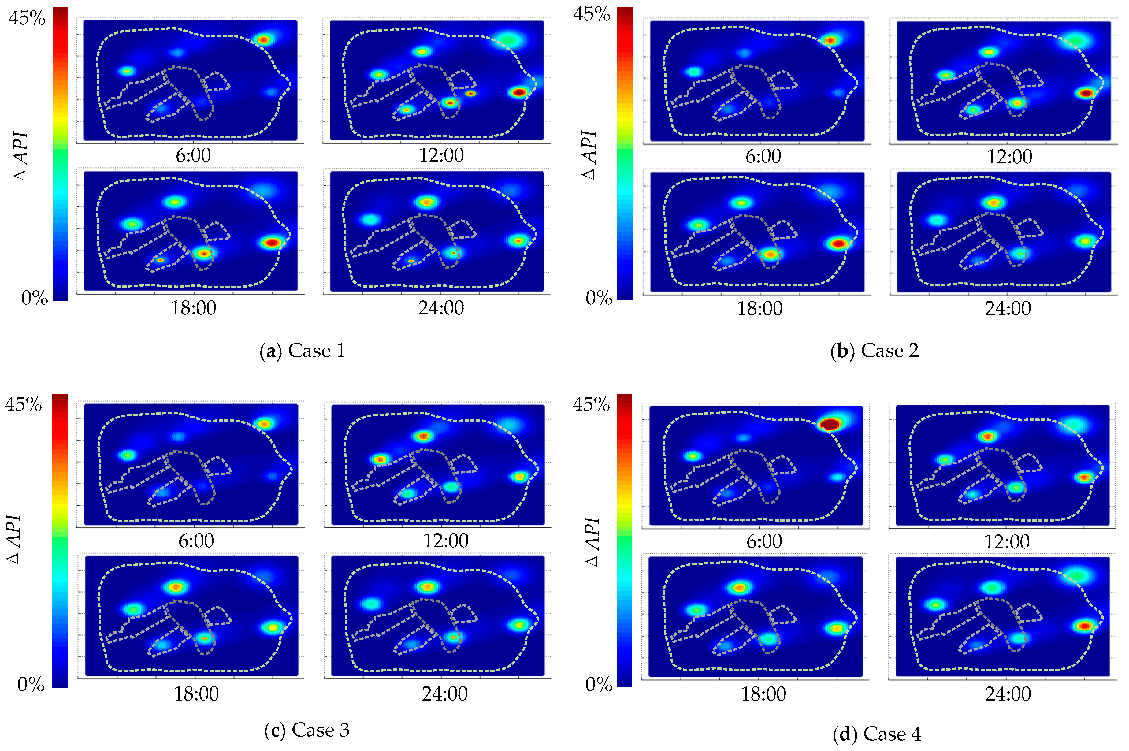
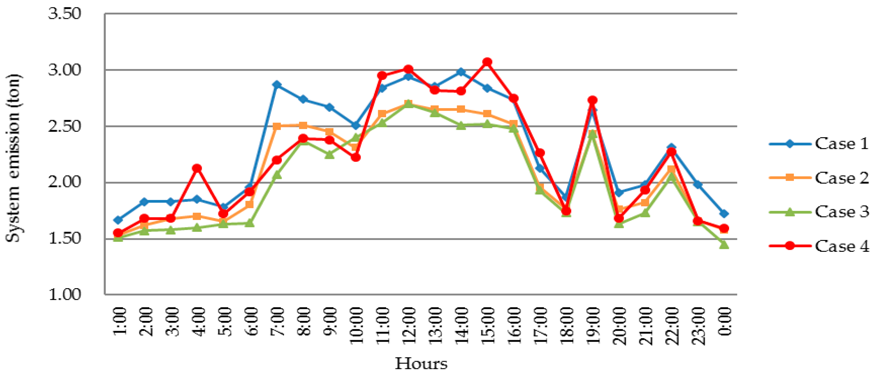
• Even with integration of wind power, the API constraints are still necessary in the dispatch model to mitigate air quality deterioration. For example, in Table 1 in R1, C_av in Case 2 is only 0.4% lower than Case 1, while C_av in Case 4 is 16.6% lower than Case 1. Although Case 2 decreases its fuel consumption because of less power demand from coal-fired units, it fails to effectively mitigate regional air quality degradation.
• The dispatch minimizing total emissions may encourage emission reductions at wrong locations and times regarding regional air quality control. In Table 1 in R1, C_av and C_pk in Case 4 are 9.5% and 12.7% lower than Case 3, respectively. This justifies that both weather conditions and geographical distribution of system are critical in environmental dispatch.
• The proposed Eco-SCUC takes advantage of wind generation and API constraints, and it can cost-effectively alleviate air quality deterioration for densely populated regions. Via shifting generation among units, the Eco-SCUC succeeds in balancing regional air quality saturation level. Although the Eco-SCUC improves regional air quality at a cost of slight increase of total costs and emissions, it can significantly reduce the person-hour exposure to severe air pollution, which is beneficial to human and environmental health.

We examine the effectiveness of the model with respect to differentiated API expectations with and without wind power. API expectation (API_E,tj) refers to the expected value of API as expressed in Equation (9). When the city tightens its air quality control, API_E,tj can be set to lower values; when the city loosens its control, API_E,tj can be set to higher values. We adjust API_E,tj from 50% to 200%.

Figure 12 shows the resulting C_av and C_pk in R1 under the Eco-SCUC, respectively. As API_E,tj decreases, the model tightens control on emissions, both C_av and C_pk drop. This demonstrates that the decrease of API_E,tj helps improve regional air quality. Especially during extreme haze-fog periods, API_E,tj could be set to relatively low value to cope with bad weather. Moreover, Figure 12 proves that the Eco-SCUC with wind power is more effective than the counterpart without wind power in reducing regional pollutant concentrations.

5.3. Discussion

This paper links regional API with electricity generation scheduling. The proposed Eco-SCUC is a useful step towards alleviating the environmental dilemma in the power sector, as it enforces differentiated API constraints above which human and ecosystem health faces severe challenges. Based on the case studies, several potential policy implementations can be drawn:

• Environmental or ecological taxes can be imposed to power plants based on the violation of API constraints. In the Eco-SCUC, the violation of API constraint can be directly linked to the ecosystem or human health damages. This solves the problem that the impact of coal-fired power plants on regional air quality cannot be quantitatively analyzed.
• Air quality compensation mechanism can be implemented by the government to press the power plants to adjust their generation in response to regional air quality. The Eco-SCUC helps calculate the compensated amount based on regional API changes.
• The developing cyber-physical system (CPS) technologies enable power grid corporations to expand their ancillary services to include API-associated regulations, thereby improving regional air quality.

6. Conclusions

This paper proposes an Eco-SCUC model addressing regional air quality management via shifting generation among units. An API index is defined for evaluating regional air pollutant saturation levels and is calculated based on a Gaussian puff dispersion model, geographically-differentiated AEC, and forecasted weather conditions. API constraints are formulated according to the differentiated impacts of coal-fired units on regional air quality and integrated into a SCUC model. Stochastic optimization is applied to accommodate volatile wind power; as such the benefits of wind power for air quality control are estimated. The test results demonstrate that the model can cost-effectively prevent air quality deterioration in densely-populated regions and reduce the person-hours exposed to severe air pollution.

Future studies will focus on the investigation of chemical conversion from primary pollutants to secondary pollutants and its integration into the Eco-SCUC model.

References

1. Zhao, Y.; Wang, S.; Duan, L.; Lei, Y.; Cao, P.; Hao, J. Primary air pollutant emissions of coal-fired power plants in China: Current status and future prediction. Atmos. Environ. 2008, 42, 8442–8452. [Google Scholar] [CrossRef]
2. Li, X.; Chen, X.; Yuan, X.; Zeng, G.; León, T.; Liang, J.; Chen, G.; Yuan, X. Characteristics of particulate pollution (PM2.5 and PM10) and their spacescale-dependent relationships with meteorological elements in China. Sustainability 2017, 9, 2330. [Google Scholar] [CrossRef]
3. Zhao, B.; Wang, S.; Dong, X.; Wang, J.; Duan, L.; Fu, X.; Hao, J.; Fu, J. Environmental effects of the recent emission changes in China: Implications for particulate matter pollution and soil acidification. Environ. Res. Lett. 2013, 8, 024031. [Google Scholar] [CrossRef]
4. Zhou, Q.; Yabar, H.; Mizunoya, T.; Higano, Y. Evaluation of integrated air pollution and climate change policies: Case study in the thermal power sector in Chongqing City, China. Sustainability 2017, 9, 1741. [Google Scholar] [CrossRef]
5. Chen, L.; Shi, M.; Li, S.; Gao, S.; Zhang, H.; Sun, Y.; Mao, J.; Bai, Z.; Wang, Z.; Zhou, J. Quantifying public health benefits of environmental strategy of PM2.5 air quality management in Beijing-Tianjin-Hebei region, China. J. Environ. Sci. 2017, 57, 33–40. [Google Scholar] [CrossRef] [PubMed]
6. Pretorious, I.; Piketh, S.; Burger, R. Emissions management and health exposure: Should all power stations be treated equal? Air Qual. Atmos. Health 2017, 10, 509–520. [Google Scholar] [CrossRef]
7. Song, C.; He, J.; Wu, L.; Jin, T.; Chen, X.; Li, R.; Ren, P.; Zhang, L.; Mao, H. Health burden attributable to ambient PM2.5 in China. Environ. Pollut. 2017, 223, 575–586. [Google Scholar] [CrossRef] [PubMed]
8. Li, L.; Liu, D. Study on an air quality evaluation model for Beijing city under haze-fog pollution based on new ambient air quality standards. Int. J. Environ. Res. Public Health 2014, 11, 8909–8923. [Google Scholar] [CrossRef] [PubMed]
9. Li, L.; Tang, D.; Kong, Y.; Yang, Y.; Liu, D. Spatial analysis of haze–fog pollution in China. Energy Environ. 2016, 27, 726–740. [Google Scholar] [CrossRef]
10. Zhao, H.; Ma, W.; Dong, H.; Jiang, P. Analysis of co-effects on air pollutants and CO2 emissions generated by end-of-pipe measures of pollution control in China’s coal-fired power plants. Sustainability 2017, 9, 499. [Google Scholar] [CrossRef]
11. Mollahassani-Pour, M.; Rashidinejad, M.; Abdollahi, A. Appraisal of eco-friendly preventive maintenance scheduling strategy impacts on GHG emissions mitigation in smart grids. J. Clean. Prod. 2017, 143, 212–223. [Google Scholar] [CrossRef]
12. Chinese Coal-Fired Electricity Generation Expected to Flatten as Mix Shifts to Renewables. Available online: https://www.eia.gov/todayinenergy/detail.php?id=33092 (accessed on 29 September 2017).
13. Wang, R.; Wang, J.; Guan, Y. Robust unit commitment with wind power and pumped storage hydro. IEEE Trans. Power Syst. 2012, 27, 800–810. [Google Scholar] [CrossRef]
14. Xu, Q.; Ding, Y.; Zheng, A. An optimal dispatch model of wind-integrated power system considering demand response and reliability. Sustainability 2017, 9, 758. [Google Scholar] [CrossRef]
15. Liu, X.; Xu, W. Minimum emission dispatch constrained by stochastic wind power availability and cost. IEEE Trans. Power Syst. 2010, 25, 1705–1713. [Google Scholar] [CrossRef]
16. Lyu, X.; Shi, A. Research on the renewable energy industry financing efficiency assessment and mode selection. Sustainability 2018, 10, 222. [Google Scholar] [CrossRef]
17. Wang, X.; Gong, Y.; Jiang, C. Regional carbon emission management based on probabilistic power flow with correlated stochastic variables. IEEE Trans. Power Syst. 2015, 30, 1094–1103. [Google Scholar] [CrossRef]
18. Wang, Y.; Huang, Y.; Wang, Y.; Li, F.; Zhang, Y.; Tian, C. Operation optimization in a smart micro-grid in the presence of distributed generation and demand response. Sustainability 2018, 10, 847. [Google Scholar] [CrossRef]
19. Zhu, Z.; Liu, D.; Liao, Q.; Tang, F.; Zhang, J.; Jiang, H. Optimal power scheduling for a medium voltage AC/DC hybrid distribution network. Sustainability 2018, 10, 318. [Google Scholar] [CrossRef]
20. Wei, W.; Liu, F.; Wang, J.; Chen, L.; Mei, S.; Yuan, T. Robust environmental-economic dispatch incorporating wind power generation and carbon capture plants. Appl. Energy 2016, 183, 674–684. [Google Scholar] [CrossRef]
21. Zhang, N.; Hu, Z.; Dai, D.; Dang, S.; Yao, M.; Zhou, Y. Unit commitment model in smart grid environment considering carbon emissions trading. IEEE Trans. Smart Grid 2016, 7, 420–427. [Google Scholar] [CrossRef]
22. Abdollahi, A.; Moghaddam, M.P.; Rashidinejad, M.; Sheikh-El-Eslami, M.K. Investigation of economic and environmental-driven demand response measures incorporating UC. IEEE Trans. Smart Grid 2012, 3, 12–25. [Google Scholar] [CrossRef]
23. Zhao, C.; Wang, J.; Watson, J.; Guan, Y. Multi-stage robust unit commitment considering wind and demand response uncertainties. IEEE Trans. Power Syst. 2013, 28, 2708–2717. [Google Scholar] [CrossRef]
24. Shi, N.; Luo, Y. Energy storage system sizing based on a reliability assessment of power systems integrated with wind power. Sustainability 2017, 9, 395. [Google Scholar] [CrossRef]
25. Mou, D. Wind power development and energy storage under China’s electricity market reform—A case study of Fujian Province. Sustainability 2018, 10, 298. [Google Scholar] [CrossRef]
26. Ban, M.; Yu, J. Procedural simulation method for aggregating charging load model of private electric vehicle cluster. J. Mod. Power Syst. Clean Energy 2015, 3, 170–179. [Google Scholar] [CrossRef]
27. Ye, J.; Yuan, R. Integrated natural gas, heat, and power dispatch considering wind power and power-to-gas. Sustainability 2017, 9, 602. [Google Scholar] [CrossRef]
28. Ban, M.; Yu, J.; Shalidehpour, M.; Yao, Y. Integration of power-to-hydrogen in day-ahead security-constrained unit commitment with high wind penetration. J. Mod. Power Syst. Clean Energy 2017, 5, 337–349. [Google Scholar] [CrossRef]
29. Zhou, Y.; Levy, J.I.; Evans, J.S.; Hammitt, J.K. The influence of geographic location on population exposure to emissions from power plants throughout China. Environ. Int. 2006, 32, 365–373. [Google Scholar] [CrossRef] [PubMed]
30. Cao, X.; Roy, G.; Hurley, W.J.; Andrews, W.S. Dispersion coefficients for Gaussian puff models. Bound.-Layer Meteorol. 2011, 139, 487–500. [Google Scholar] [CrossRef]
31. Fann, N.; Fulcher, C.M.; Hubbell, B.J. The influence of location, source, and emission type in estimates of the human health benefits of reducing a ton of air pollution. Air Qual. Atmos. Health 2009, 2, 169–176. [Google Scholar] [CrossRef] [PubMed]
32. Sullivan, R.L.; Hackett, D.F. Air quality control using a minimum pollution-dispatching algorithm. Environ. Sci. Technol. 1973, 7, 1019–1022. [Google Scholar] [CrossRef] [PubMed]
33. Schweizer, P.F. Determining optimal fuel mix for environmental dispatch. IEEE Trans. Autom. Control 1974, 19, 534–537. [Google Scholar] [CrossRef]
34. Chu, K.; Jamshidi, M.; Levitan, R.E. An approach to on-line power dispatch with ambient air pollution constraints. IEEE Trans. Autom. Control 1977, 22, 385–396. [Google Scholar] [CrossRef]
35. Levy, J.I.; Spengler, J.D.; Hlinka, D.; Sullivan, D.; Moon, D. Using CALPUFF to evaluate the impacts of power plant emissions in Illinois: Model sensitivity and implications. Atmos. Environ. 2002, 36, 1063–1075. [Google Scholar] [CrossRef]
36. Napelenok, S.L.; Cohan, D.S.; Hu, Y.; Russell, A.G. Decoupled direct 3D sensitivity analysis for particulate matter (DDM-3D/PM). Atmos. Environ. 2006, 40, 6112–6121. [Google Scholar] [CrossRef]
37. Duan, L.; Xie, S.; Zhou, Z.; Ye, X.; Hao, J. Calculation and mapping of critical loads for S, N and Acidity in China. Water Air Soil Pollut. 2001, 130, 1199–1204. [Google Scholar] [CrossRef]
38. Porter, E.; Blett, T.; Potter, D.U.; Huber, C. Protecting resources on Federal Lands: Implications of critical loads for atmospheric deposition of nitrogen and sulfur. Bioscience 2005, 55, 603–612. [Google Scholar] [CrossRef]
39. Pingxing, L.; Jie, F. Regional ecological vulnerability assessment of the Guangxi Xijiang River Economic Belt in Southwest China with VSD model. J. Resour. Ecol. 2014, 5, 163–170. [Google Scholar] [CrossRef]
40. Wang, M.; Liu, J.; Wang, J.; Zhao, G. Ecological footprint and major driving forces in West Jilin Province, Northeast China. Chin. Geogr. Sci. 2010, 20, 434–441. [Google Scholar] [CrossRef]
41. Yanxi, C. Study of the Atmospheric Environment Capacity in Harbin City. Master’s Thesis, Harbin Institute of Technology, Harbin, China, 2015. (In Chinese). [Google Scholar]
42. Zhou, Y.; Zhou, J. Urban atmospheric environmental capacity and atmospheric environmental carrying capacity constrained by GDP–PM2.5. Ecol. Indic. 2017, 73, 637–652. [Google Scholar] [CrossRef]
43. Xu, D.; Wang, Y.; Zhu, R. Atmospheric environmental capacity and urban atmospheric load in mainland China. Sci. China Earth Sci. 2018, 61, 33–46. [Google Scholar] [CrossRef]
44. Zoras, S.; Triantafyllou, A.G.; Deligiorgi, D. Atmospheric stability and PM10 concentrations at far distance from elevated point sources in complex terrain: Worst-case episode study. J. Environ. Manag. 2006, 80, 295–302. [Google Scholar] [CrossRef] [PubMed]
45. An, X.; Zuo, H.; Chen, L. Atmospheric environmental capacity of SO2 in winter over Lanzhou in China: A case study. Adv. Atmos. Sci. 2007, 24, 688–699. [Google Scholar] [CrossRef]
46. Air Quality Index for Harbin City. Available online: http://www.pm25.in/haerbin (accessed on 24 January 2018).
47. Wang, J.; Shahidehpour, M.; Li, Z. Security-constrained unit commitment with volatile wind power generation. IEEE Trans. Power Syst. 2008, 23, 1319–1327. [Google Scholar] [CrossRef]
48. Masters, G.M. Renewable and Efficient Electric Power Systems; Wiley: New York, NY, USA, 2004. [Google Scholar]
49. Karki, R.; Patel, J. Reliability assessment of a wind power delivery system. Proc. Inst. Mech. Eng. Part O J. Risk Reliab. 2008, 223, 51–58. [Google Scholar] [CrossRef]
50. Hetzer, J.; Yu, D.C.; Bhattarai, K. An economic dispatch model incorporating wind power. IEEE Trans. Energy Convers. 2008, 23, 603–611. [Google Scholar] [CrossRef]
51. Hajipour, E.; Bozorg, M.; Fotuhi-Firuzabad, M. Stochastic capacity expansion planning of remote microgrids with wind farms and energy storage. IEEE Trans. Sustain. Energy 2015, 6, 491–498. [Google Scholar] [CrossRef]
52. Wu, L.; Shahidehpour, M.; Li, T. Stochastic security-constrained unit commitment. IEEE Trans. Power Syst. 2007, 22, 800–811. [Google Scholar] [CrossRef]
53. Lopez, J.A.; Ceciliano-Meza, J.L.; Moya, I.G.; Gomez, R.N. A MIQCP formulation to solve the unit commitment problem for large-scale power systems. Int. J. Electr. Power 2012, 36, 68–75. [Google Scholar] [CrossRef]
Figure 1. Cyber-physical framework of the proposed Eco-SCUC. Coal-fired power plant A and B are assumed to be identical near-city power plants. Remote power plants represent power plants near coal-mines which are located in sparsely-populated or unmanned regions. Blue dots represent air quality ground stations; and blue lines and green lines represent inputs and outputs for the dispatching center.
Sustainability 10 01433 g001
Figure 2. Methodology of formulating differentiated API constraints. Meteorological data are inputs for Gaussian puff model, and the generation-associated concentrations Ci are calculated; the regional threshold concentrations CT are derived according to AEC model. Based on Ci and CT, regional APIs are obtained and differentiated constraints are formed according to regional background API value.
Sustainability 10 01433 g002
Figure 3. Top view of the Gaussian puff dispersion model.
Sustainability 10 01433 g003
Figure 4. (a) SO2 threshold concentration and (b) API of SO2 by administrative-district-level of one city in Northeast China. Daily-average concentration data are from [46].
Sustainability 10 01433 g004
Figure 5. CDF and PDF of wind generation PW: (a) CDF of PW; (b) PDF of PW. Assumptions: c = 15, vin = 5 m/s, vout = 45 m/s, vr = 15 m/s, k = 1.2, 1.7, or 2.2. CDF includes both discrete probabilities (marked as colorful dots) and continuous probabilities, while PDF only contains continuous portions.
Sustainability 10 01433 g005
Figure 6. Diagram of the Eco-SCUC model. Blue represents the electricity network; red represents the environment network; the full lines represent physical structure; and the dotted lines represent data and information.
Sustainability 10 01433 g006
Figure 7. Eco-SCUC solution methodology. Part I includes the master UC problem and hourly network security check sub-problem; Part II includes the wind power scenario feasibility check sub-problem.
Sustainability 10 01433 g007
Figure 8. Geographical distribution of unit G1–G6 and region R1–R5. R1 represents the city center; R1–R4 represent the densely-populated regions; and R5 represents the sparsely-populated region.
Sustainability 10 01433 g008
Figure 9. Hourly generation results for G1–G6 in Cases 1–4.
Sustainability 10 01433 g009
Figure 10. Hourly system emissions in Cases 1–4.
Sustainability 10 01433 g010
Figure 11. Distribution of API increments (ΔAPI) in Cases 1–4. Four representative hours of the day are chosen: 6:00, 12:00, 18:00, and 24:00. ΔAPI refers to the contribution of coal units on regional API. White dotted lines represent the five regions as shown in Figure 8.
Sustainability 10 01433 g011
Figure 12. (a) Cav and (b) Cpk of SO2 in R1 under the Eco-SCUC with respect to differentiated APIE,tj, with and without wind power.
Sustainability 10 01433 g012