Determinants of Agricultural Diversification in a Hotspot Area: Evidence from Colonist and Indigenous Communities in the Sumaco Biosphere Reserve, Ecuadorian Amazon

Abstract

With data from a household survey covering migrant settlers and indigenous (Kichwa) communities in the Sumaco Biosphere Reserve (SBR), this study analyses the drivers of agricultural diversification/specialisation, focusing on the role of ethnicity and the livelihood strategies (LS) they follow. Data were collected using the Poverty and Environment Network methodology of the Center for International Forestry Research (CIFOR-PEN). In order to establish the drivers of agricultural diversification, the number of crops and the Shannon index of crops areas were used as the dependent variables in ordinary least square (OLS) models, while a multinomial logit model (MLM) was used to assess a household’s degree of diversification. The results of the OLS regression provides evidence supporting the notion that households, with Livestock-based and Wage-based livelihood strategies (LS) are less diversified and more specialized than households with Crop-based LS. Ethnicity has a positive and significant effect on agricultural diversification, with Kichwa farms more diversified than those of their migrant colonist counterparts. The results of the multinomial logit model (MLM) show that large Kichwa households, with Crop-based and Forest-based LS are more likely to adopt a highly diversified agricultural strategy. Based on these findings, we recommend a redirection of agricultural incentives, towards the adoption of diversified agricultural systems, as a strategy to promote more sustainable production systems in the Ecuadorian Amazon Region.

1. Introduction

Worldwide, almost half of the total usable land is now pastoral or intensive agriculture in use [1]. These systems produce about half of the world’s food and are essential in addressing rural food insecurity and poverty in developing countries [2]. However, these systems are also considered to be the major cause of the continuous loss of tropical forests and degradation of tropical ecosystems [3] due to the expansion of the agricultural frontier [4,5,6]. Such land use changes have been responsible for around 12% of global CO₂ emissions over the last decade (2007–2016) [7]. Most of these estimations have been made using a large database with a global prediction subject to a high level of uncertainty. Whilst the problems are global, solutions must be treated at local, regional and global levels [1]. Hence, one of the principal challenges for researchers is increasing agricultural production without damaging the environment [4,5,6] and the facilitation of policy recommendation. In this sense, agricultural diversification is frequently identified as a potential strategy that contributes towards more sustainable and competitive commodities, increasing rural incomes, generating on-farm employment and alleviating poverty.

Hence, this paper uses the concept of Joshi and colleagues who consider agricultural diversification as “a shift of resources from one crop (or livestock) to a larger mix of crops and livestock, keeping in view the varying nature of risks and expected returns from each crop/livestock activity and adjusting it in such a way that it leads to optimum portfolio of income” [8] (p. 2457). In this context, several authors argue that diversification could improve risk management and alleviate poverty, economic crises, internal/external shocks [9,10,11,12,13], natural disturbances and climate change [6,14,15] while increasing food security and dietary diversity [14,16]. Despite the increase of industrialization in agriculture, millions of small-scale famers in rural areas still use diversified agricultural systems to produce sustained yields for their subsistence needs [14,17]. Previous local empirical studies have examined agricultural diversification and its relationship with household livelihoods in a wider context, for example, by examining poverty alleviation [10] and agricultural risk management [18,19]. Some authors also reported differences concerning the determinants of agricultural diversification. For instance, Tung [20] found that larger agricultural areas favour specialization rather than diversification, while McNamara and Weiss [21] state the opposite effect. Babatunde and Qaim [22] conclude that diversification increases with overall household income, whilst Jones et al. [16] suggest that wealthier households in Malawi accomplish a more diversified production without expanding the cultivated land area. On the other hand, a study conducted in a semi-arid agricultural system in Kenya outlines the influence of precipitation on crop diversity [15]. Furthermore, Bartolini and Brunori [23] observe that proximity to popular tourist areas and urban markets plays an important role in shaping on-farm diversity income. Such studies show that agricultural diversity is affected by a wide range of variables and show the need to conduct case studies in particular areas.

Several approaches are available to measure agricultural diversification. In many cases, the use of proportional abundance measures of diversity methods, for example, Simpson [16,20,24], Hirfendahl [22,25,26] and the Shannon equitability index of diversity [27,28,29] are appropriate. These methodologies are suitable for determining agricultural diversification or specialization and have usually been applied in economic literature. However, for the purpose of calculating the diversification of the crop area, we used the Shannon diversity index (H_{crop_area}). To classify the degree of diversification, we used the Shannon equitability index for crop area (E_{crop_area}). In the latter, a zero value indicates specialization and values greater than zero denote some degree of diversification [25]. In conjunction, we also used the simple richness index method that measures the total number of different crops a household grows, which is used in several studies [10,15,21,23]. In addition, to estimate the determinants of agricultural area diversification, a number of methodologies have been applied. We employed Ordinary Least Squares (OLS) since the outcomes have a small proportion of zero values as a fraction of the number of crops within the whole sample in our study area and a multiple regression using OLS is appropriate in these cases [16,25,30]. Moreover, to analyse the factors associated with the households’ degree of diversification choice, a Multinomial Logit Model (MLM) was employed.

In Ecuador, one of the world’s most mega-diverse countries [31,32], about 90% of the deforested area in the last two decades was converted somehow into agricultural areas, as a result of forests converted into crops and pastures [33]. The Ecuadorian Amazon Region (EAR) has experienced this same pattern of an expanding agricultural frontier. The EAR is a region that comprises about 48% of Ecuador’s total surface area, with a population growth of 5.1% (up to the year 2010). The population is predominantly rural, with around 60 in extensive agricultural production systems [34]. It is estimated that throughout the EAR, there are around one million hectares of pastureland [35]. The Ecuadorian government in its Agenda for Productive Transformation in the Amazon (ATPA, for its Spanish acronym) has aimed at reducing the area of pastures by converting them into more sustainable production systems through reforestation and natural restoration. In these contexts, research on local production systems and traditional knowledge linked to sustainable agriculture is urgently needed in the EAR.

Conducting a study at a household level, in the transition and buffer zone of the Sumaco Biosphere Reserve in the EAR (Figure 1), we depart from the hypothesis that agricultural diversity is affected by ethnicity and the livelihood strategies (LS) that a household pursues with consequences on socioeconomic variables. Hence, this paper focuses on issues of agricultural diversification in a biological hotspot area inhabited by indigenous populations and migrant-settlers 50 years after colonization. The following questions are assessed: (i) How does diversification relate to livelihood strategies in terms of agricultural area and income sources? and (ii) What are the socioeconomic factors related to higher diversification?

Hence, this study aimed at (a) examining the agriculture diversification by LS using the Shannon diversity index of agriculture (Crops and livestock); and (b) evaluating the effect of LS and ethnicity on the degree of agriculture diversification using a range of high, medium and low diversification determined from the Shannon equitable index. Finally, as a basis for potential policy implications we discuss if agricultural diversification in rural livelihood strategies could lead to more sustainable production systems.

The paper is organized as follows: the next section briefly describes the material and methods, including the study area and the statistical methods used to analyse the effect of livelihood strategies, ethnicity and other socioeconomic factors affecting a household’s agricultural diversification. Next, the results are described followed by the discussion, policy implications and main conclusions.

2. Materials and Methods

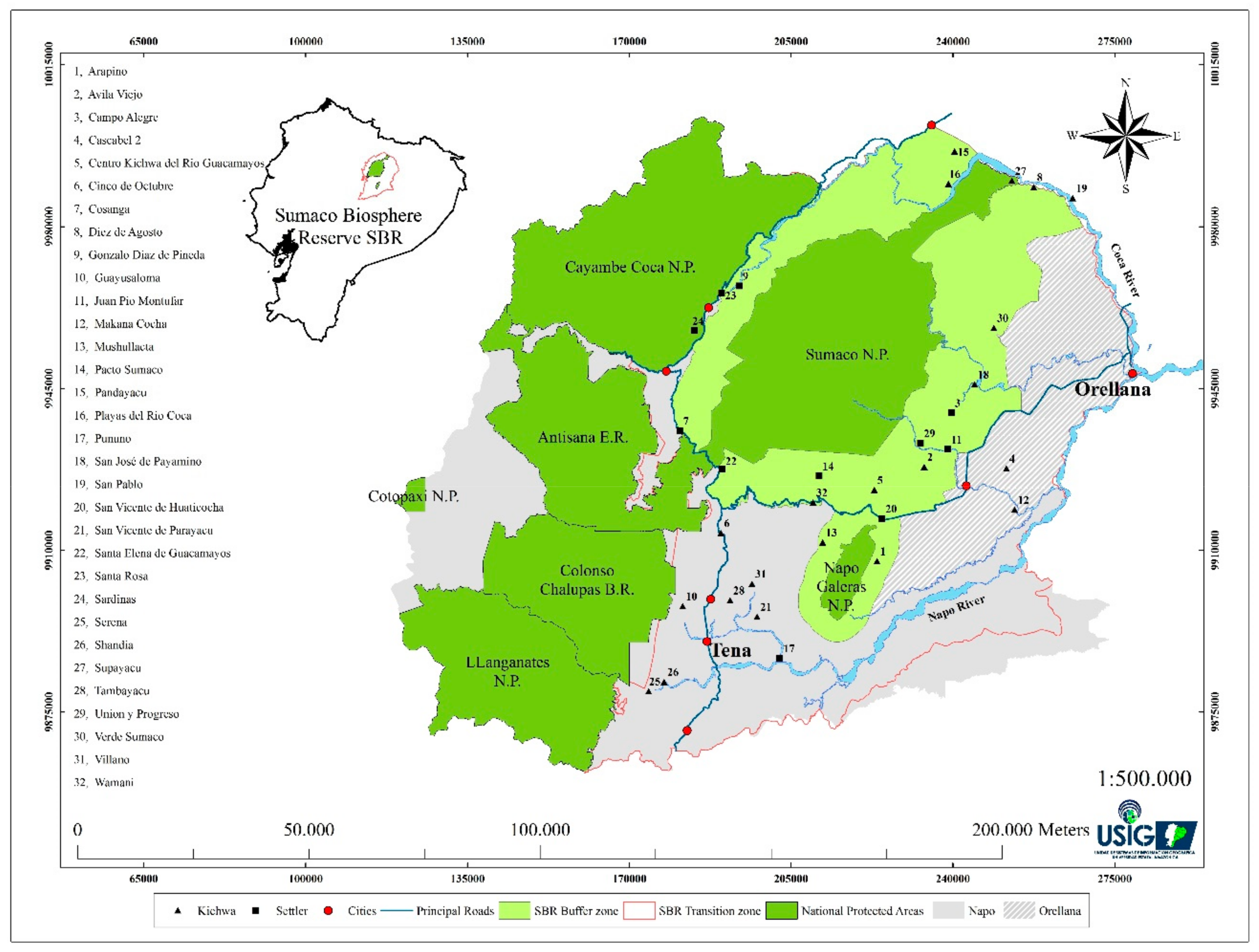
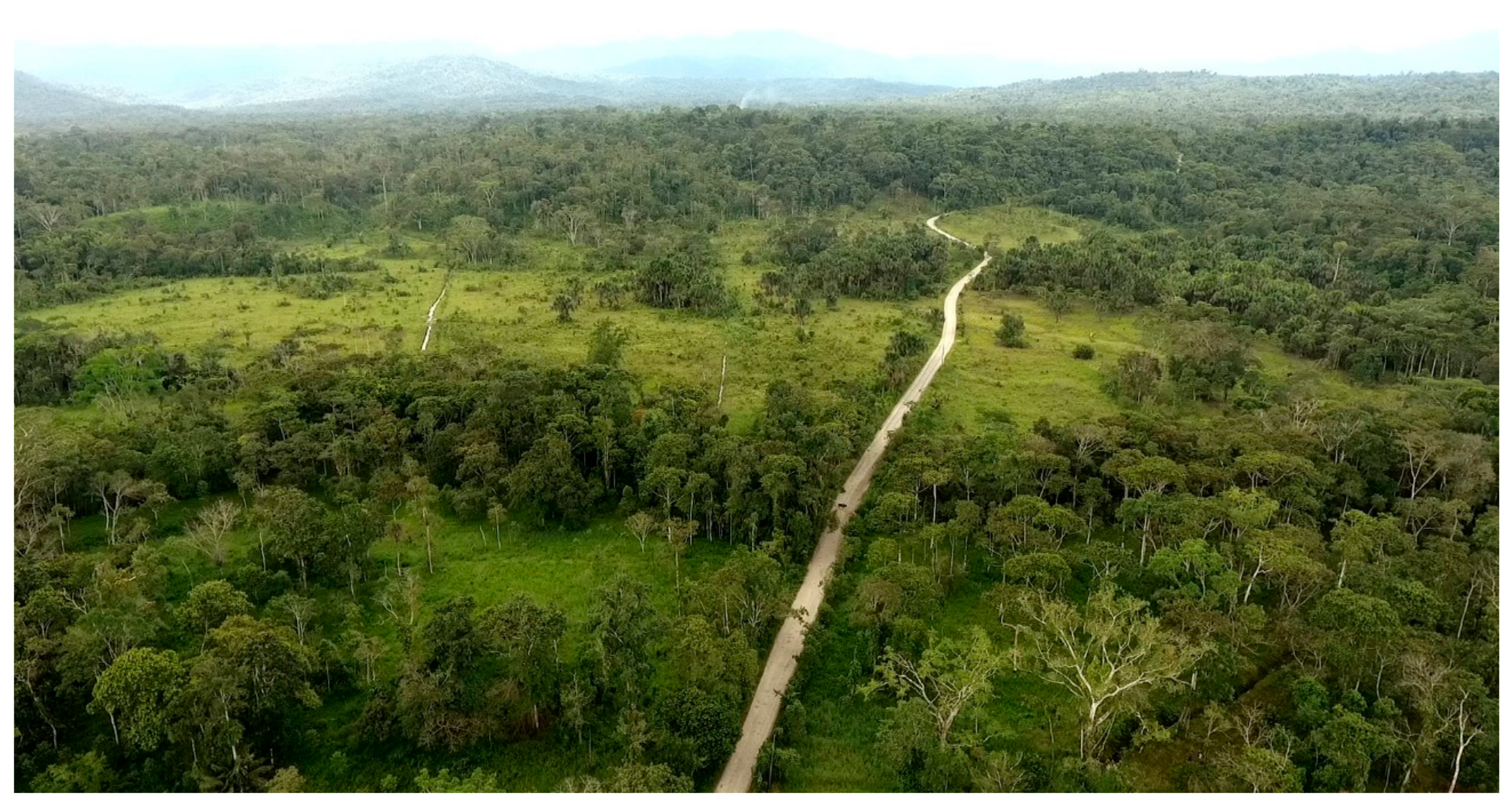
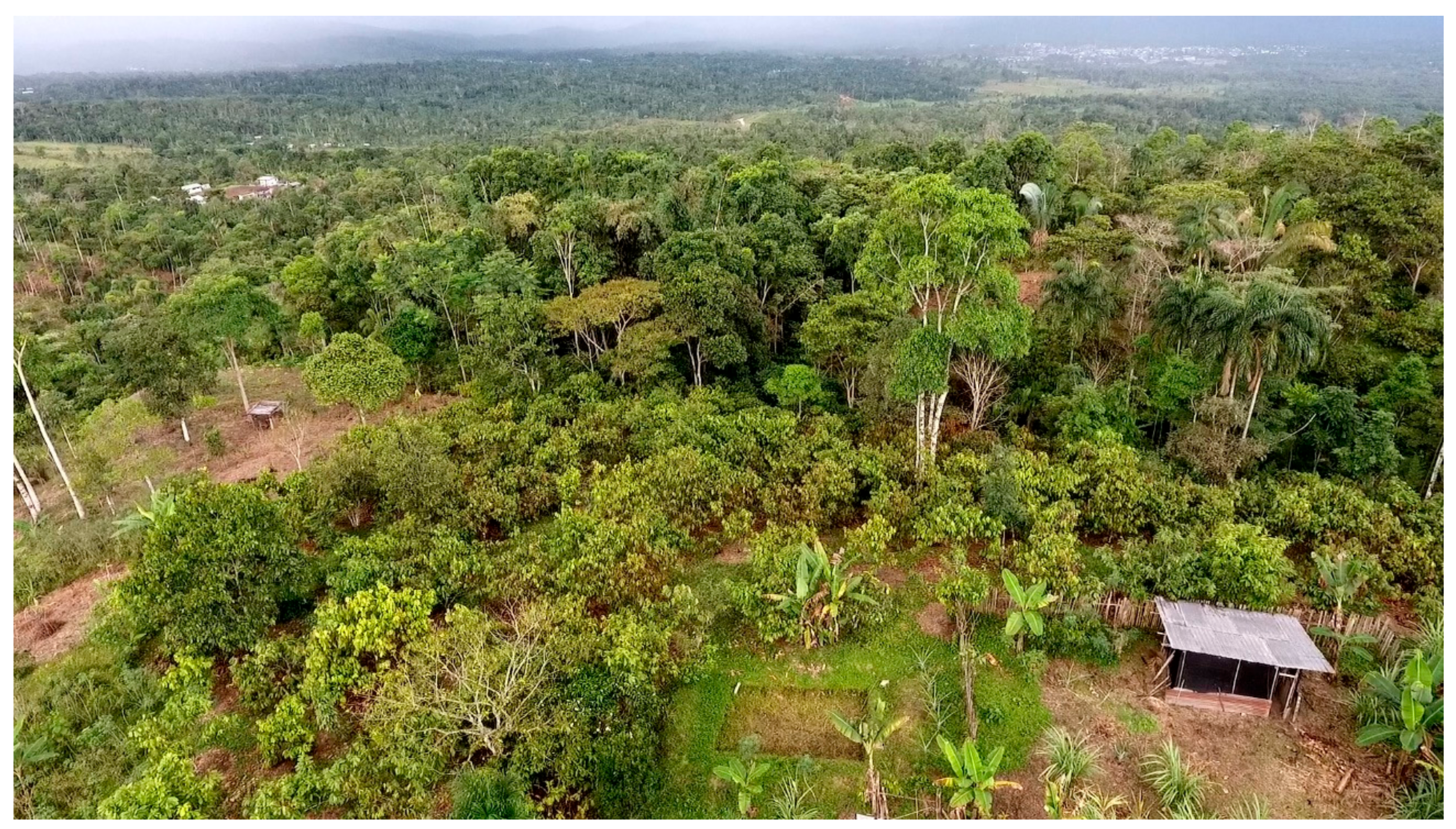
2.1. Study Area and Agricultural Contexts

The northern and central part of the EAR, prior the petroleum era, was populated by indigenous people and very few colonists, with the forest landscape largely intact [36]. Since the discovery of crude oil in 1967, this region began to be occupied by agricultural settler families [37] who migrated from other rural areas of Ecuador [38,39], then roads were laid down for the oil exploitation and the Agrarian Reform Laws were enacted (1964 and 1972), which stimulated the colonization of Amazonian forest land [37,39]. These factors have promoted an intense process of land use change that generally follows similar productive and survival strategies, including the cultivation of subsistence and cash crops, pasture to raise cattle [40,41,42] and timber logging [39,41,43], as well as land fragmentation due to population growth [38,40]. However, during the last two decades, Ecuador has made efforts to encourage sustainable development. In 2008, Ecuador became the first country to grant legal rights to nature, with the aim of improving livelihoods and agricultural production systems in the EAR [42] and in 2011 with the government announced the ATPA, which promotes a sustainable productive transformation [35].

This study was conducted in the buffer and transition zones of the Sumaco Biosphere Reserve (SBR), where around one million hectares of tropical forest were established as a biosphere reserve by UNESCO’s Man and Biosphere program (Biosphere reserve are “areas of terrestrial and coastal/marine ecosystems or a combination thereof, which are internationally recognized within the framework of UNESCO’s Programme on Man and Biosphere (MAB)’ (Statutory Framework of World Network of Biosphere Reserves”) in 2000. This site was officially recognized by the Ecuadorian government in 2002. Its core area of conservation is the Sumaco Napo Galeras National Park (PNSNG), which is comprised of 205,751 ha [44]. The SBR is located in the central northern EAR. The SBR is spread between the provinces Napo, Orellana and Sucumbíos and borders four important protected areas: Cayambe Coca National Park, Llanganates National Park, Antisana Ecological Reserve and Colonso-Chalupas Biological Reserve (Figure 1).

According to the Sevilla Strategy, each biosphere reserve serves three complementary functions: “a conservation function, to preserve genetic resources, species, ecosystem and landscapes; a development function, to foster sustainable economic and human development and a logistic support function, to support demonstration projects, environmental education and training and research and monitoring related to local, national and global issues of conservation and sustainable development” [45] (p. 4). Thus, the buffer and transition zones fulfils the development and logistic support functions respectively and this is where the communities within the SBR are located (Figure 1).

The SBR is part of an important ecosystem in the Amazonian foothills, located in an altitudinal gradient from tropical rain forest, 300 to 3732 m above sea level at the Sumaco volcano’s summit. The area is part of the hotspot called the ‘Uplands of Western Amazonia’ [31,46]. Nevertheless, like many other areas of high biodiversity which are under threat from habitat destruction [32], the SBR also faces high rates of deforestation and land use change. From 2008 to 2013, the SBR lost 93,853 hectares of native forest [47]. This accounts for a 10.8% shift to other land uses over a period of 5 years, with a deforestation rate of 2.16% in the whole SBR. This change exemplifies a strong conversion from forests to land for pasture, crops and fallow [47].

Currently, the human population in the SBR is approximately 206,000 and the average annual growth rate is 3% [47]. Most of inhabitants are indigenous Kichwa and less than 40% are migrant settlers.

For most migrant settlers and some Kichwa populations in the SBR, the agricultural systems are made up mainly of cash crops, such as pasture for cattle (Figure 2), cocoa (Theobroma cacao L.), coffee (Coffea canephora Pierre ex A. Froehner), maize (Zea mays L.) and naranjilla (Solanum quitoense Lam.), in addition to staple crops, such as yucca (Manihot esculenta Crantz), plantain (Musa paradisiaca L.) and peach palm (Bactris gasipaes Kunth) [48,49,50,51]. These trends are fairly similar to those found in the northern Ecuadorian Amazon Region [37,39,41] and by Vasco et al. [52] and Lerner et al. [53] in the central and southern Ecuadorian Amazon Region, respectively.

For most of the Kichwa population, the “Chakra” system is the most common traditional agroforestry system [48,51,54,55]. It is characterized by its high level of biodiversity and high number of timber-yielding and fruit trees [48,51,56,57]. The chakra in the SBR is also considered a polyculture [48,56], where the principal crops are cocoa (Theobroma cacao L.), coffee (Coffea canephora Pierre ex A. Froehner) and nowadays guayusa (Ylex Guayusa Loes) [58,59]. These crops grow alongside plants used for medicine, spiritual rituals, making crafts and other consumption purposes [48], as well as together with forest trees (see Vera et al. [56]) and fruit trees for consumption and multipurpose materials (Figure 3). According to Torres and colleagues [51] there are nearly 12,500 ha of cacao cultivated in the chakra system in the buffer and transition areas of the SBR, with the size of chakra plots ranging from 0.5 to 4 ha [51].

2.2. Data Collection

This study used the Poverty and Environment Network (PEN) methodology developed by CIFOR [60]. This approach consisted of four quarterly questionnaires at a household level, two annual household surveys (separated by twelve months) and, two community-level annual surveys. The questionnaires were administered to a sample of 186 households. Households were selected in two steps. Firstly, 32 communities were randomly selected (21 Kichwa and 11 settler), accounting for 12% of the total number of communities (300) inside the buffer and transition zone of the SBR (

Table 1. Main characteristics of the communities selected for the household survey within the Sumaco Biosphere Reserve, 2008.

Community	Elevation m.a.s.l.	Ethnic Group	Population	Major Agricultural Activities
Arapino	538	Kichwa	120	Agriculture, agroforestry
Avila Viejo	596	Kichwa	400	Agriculture, agroforestry
Campo Alegre	420	Settler	490	Agriculture, cattle
Cascabel 2	343	Kichwa	300	Agriculture, timber
Centro K. Río Guacamayos	628	Kichwa	300	Agriculture, agroforestry
Cinco de Octubre	325	Kichwa	60	Agriculture, agroforestry
Cosanga	2004	Settler	700	Cattle, fish ecotourism
Diez de Agosto	377	Kichwa	80	Agriculture, agroforestry
Gonzalo Diaz de Pineda	1625	Settler	350	Cattle, monoculture
Guayusaloma	1997	Kichwa	108	Agroforestry, cattle
Juan Pio Montufar	497	Settler	700	Agriculture, timber
Makana Cocha	325	Kichwa	130	Agriculture, timber
Mushullacta	936	Kichwa	600	Agriculture, agroforestry
Pacto Sumaco	1519	Settler	600	Agroforestry, cattle
Pandayacu	472	Kichwa	550	Agriculture, agroforestry
Playas del Rio Coca	566	Kichwa	124	Agriculture, agroforestry
Pununo	414	Settler	250	Timber, Agriculture
San José de Payamino	304	Kichwa	325	Agriculture, agroforestry
San Pablo	349	Kichwa	500	Agriculture, agroforestry
San Vicente de Huaticocha	621	Settler	220	Cattle, agriculture
San Vicente de Parayacu	825	Kichwa	22	Agriculture, agroforestry
Santa Elena de Guacamayos	1646	Settler	135	Cattle, agriculture, fish
Santa Rosa	1493	Settler	350	Cattle, agriculture
Sardinas	1706	Settler	600	Cattle, agriculture
Serena	544	Kichwa	280	Agriculture, agroforestry
Shandia	514	Kichwa	320	Agriculture, agroforestry
Supayacu	395	Kichwa	55	Agriculture, agroforestry
Tambayacu	699	Kichwa	500	Agriculture, agroforestry
Union y Progreso	761	Settler	150	Agriculture, cattle
Verde Sumaco	324	Kichwa	290	Agriculture, agroforestry
Villano	821	Kichwa	370	Agriculture, agroforestry
Wamani	1174	Kichwa	700	Agroforestry, cattle

Source: Analysis from survey data PEN/RAVA—SBR, (project grant TF090577), 2008.

; Figure 1). The use of this approach ensures a fair representation of the communities and improves the robustness of the results [61]. The proportion of Kichwa and migrant settlers’ communities in our sample is consistent with that reported for the SBR as a whole (70% Kichwa and 30% migrant settlers [62]. Next, five to seven households were randomly selected in each community.

This paper is part of a collaborative research project conducted in the Amazon region seeking to understand the heterogeneity of livelihood patterns and the level of dependency on environmental resources in Amazonian contexts characterized by local or traditional populations engaged in agricultural activities. The project was implemented in 2008–2010 by a team of researchers linked to the Network for the Study of Livelihoods and Environment in the Amazon (RAVA). RAVA’s tangible objective was to generate a solid shared regional database to define which Amazonian communities rely on natural resources and on agriculture for their livelihoods. This project is also part of the PEN.

2.3. Identification of Livelihood Strategies

We adopted the livelihood strategy clusters identified by Torres et al. [42]. These authors used two multivariate techniques: (a) first a Principal Component Analysis (PCA) to reduce dimensionality using the proportion of nine income sources. The nine income variables used in the PCA were the relative earnings from: environmental resources, fishing in rivers, aquaculture (fish ponds), business activities, wages from employment, forestry uses, agricultural production, livestock production and other activities; (b) followed by an Agglomerative Hierarchical Clustering (AHC), where the first five major components resulting from the PCA were used and accounted for 70.15% of the cumulative variance of the original income data, which was considered sufficient to develop the HCA. Thus, Torres et al. [42] determined four LS, namely Forest-based, Crop-based, Livestock-based and Wage-based. In the same study, the percentage of crop land and pasture land, as well as the total income, differed significantly across the four household LS with p < 0.001. These differences are analysed in this paper, including a break-down of each crop. In addition, we analysed the effect of the four LS and ethnicity on agricultural diversification.

Additionally, two important household characteristics of LS should be considered from a previous study: (a) firstly, that the proportion of the remaining forest land was in average 64% for those households engaged in Forest-based LS, 60% for those in Crop-based LS, 53% for households in Livestock-based LS and 65% for households in Wage-based LS; (b) secondly, that off-farm income (including jobs, business and other income such as remittances or land rent) are important income sources in the SBR. These off-farm activities comprise not less than 21% of the total income of all LS and an average of around 78% for those households engaged in Wage-based LS [42].

2.4. Computing Agricultural Diversification

To measure agricultural diversification amongst the LS, we first used the number of crop areas (NCA), which involves the numbers of household crops and pasture areas. Secondly, we measured the level of agricultural crop area diversification, computing the Shannon diversity index (H_{crop_area}). This methodology is commonly used to assess species diversity [63]. The complete formula of the H applied in this paper is described as follows:

$$H_{crop\_area}=-{\sum }_{i=1}^S[({cropshare}_i)\times ln({cropshare}_i)],$$

(1)

where, S is the number of farm crop area sources and cropshare_i is the share of crop area from activity i in total household crop area. The Shannon index H_{crop_area} takes into account both the number of crops sources and their evenness. Based on this H index, the Shannon equitability index, E, is calculated as:

$$E_{crop\_area}=\left(-\frac{H_{crop\_area}}{{\sum }_{i=1}^S\left(\frac{1}{S}\ast ln(\frac{1}{S})\right)}\right)\times 100,$$

(2)

where the denominator is the maximal possible H and E ranges from 0 to 100, reflecting the share of the actual crop area diversification in relation to the maximum possible diversity of crop area.

2.5. Modelling Agricultural Diversification and Their Determinants

We used a linear regression model to examine the determinants of agricultural diversification. Ordinary least square regression shows the determinant variable for each category versus the base category (in our case, crop-based strategy). We therefore used a model with the following form:

Y_i = β X_i + ε_i

(3)

where Y is the number of crop area source (NCS) and H_{crop_area}, X is a vector of individual and household characteristics described in

Table 2. Descriptive statistics of dependent variables used in the regression models.

Variables	Nature	Description	Mean (Standard Deviation)
Dependent variable (OLS)
Hcrop_area	Continuous	Shannon diversity index of crop area	0.75 (0.5)
NCS	Continuous	Number of crop sources (Richness)	2.9 (1.6)
Dependent variable (MLM)
Household degree of crop area diversification	Categorical	Values taken from one to three based on the results of the Shannon equitable diversification status of Ecrop_area: high diversification, medium diversification and low diversification
Independent variables
Forest-based LS	Dummy	Numbers of households in forest-based LS (0/1)	36
Crop-based LS	Dummy	Numbers of households in crop-based LS (0/1)	81
Livestock-based LS	Dummy	Numbers of households in livestock-based LS (0/1)	23
Wage-based LS	Dummy	Numbers of households in wage-based LS (0/1)	46
Age head household	Continuous	Age of household head (years)	44.4 (12.1)
Household size	Continuous	Number of household members	6.6 (3.4)
Ethnicity (Kichwa)	Dummy	Household head is Kichwa (0/1)	66
Education head	Continuous	Length of formal education of household head (years)	6.2 (3.5)
Access to credit	Dummy	Households access to any type of credit (0/1)	54
Subsistence income	Continuous	Percentage of subsistence income	24.2
Remaining forest land	Continuous	Percentage of remaining forest cover on farm	46.6
Total land	Continuous	Household’s total land (ha)	28.3 (20.5)
Inside buffer zone	Continuous	Percentage of households inside the buffer zone/SBR	68
Distance city	Continuous	Time it takes to reach cities from communities (minutes)	70.1 (62.8)
Road access	Dummy	Availability of road to access village by car (0/1)	78

Notes: OLS Ordinary least square. MLM multinomial logit model. LS Livelihood strategies. (0/1) identifies dummy variables.

, β is a vector of coefficients, the direction and magnitude of which are of interest in this study and ε stands for the disturbance term.

Additionally, we used a multinomial logit model to identify the determinants of the degree of agricultural diversification. The MLM shows the determinant variables for each category versus the base category (in this case, crop-based strategy). We chose this methodology because it is appropriate for determining the influence of a selected set of explanatory variables on a dependent variable with more than two unordered outcomes [64]. In this case, the model’s dependent variable is the result of the diversification degree from the Shannon equitable indices (E_{crop_area}), with the three determined agricultural diversification levels: high diversification, medium diversification and low diversification, which accounted for fifteen independent variables (Table 2). Thus, the model was specified as the probability of occurrence of a particular degree of diversification given the independent variables. We therefore used a model of the following form:

$$\mathrm{Pr}(Y_i=K-1)=\frac{e^{\beta }K-1^{\cdot X_i}}{1+{\sum }_{k=1}^{K-1}{e}^{\beta }{k}^{\cdot X_i}},$$

(4)

where K is the number of diversity degrees (in this case three), one of which is the main level of diversification of an individual i, X is a vector of independent variables and β is a vector of coefficients the magnitude and direction of which are of fundamental interest for this study. The dependent variables are the three diversification levels. The model contained fourteen explanatory variables: forest-based LS, livestock-based LS, wage-based LS, ethnicity, age of household head, education of household head, household size, access to credit, forest land, total land, allocation, distance to city and road access (see Table 2 for a more detailed description). The average total income was not included in the model to avoid endogeneity since the four LS were developed from income percentages.

3. Results

The following section uses cross-sectional study results to examine households’ agricultural area and income distributions among four livelihoods strategies identified in the SBR. We also describe the result of the econometrics analyses, presenting relationships between variables and the determinants of agriculture diversification.

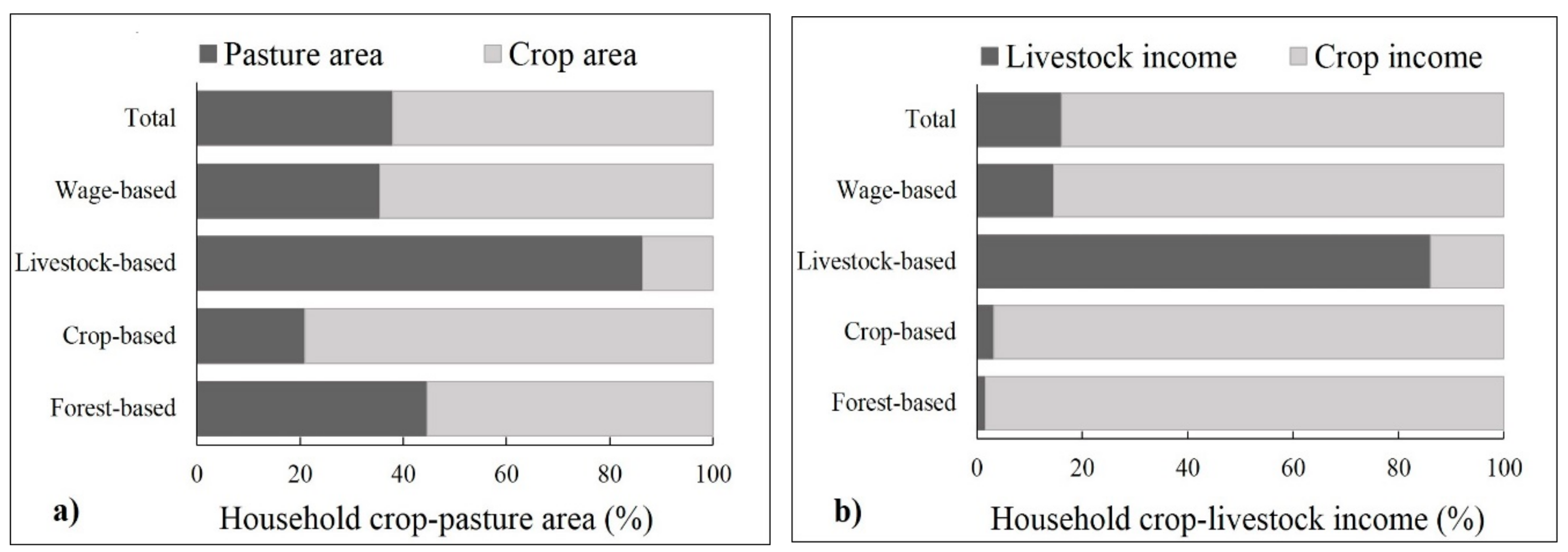
3.1. Agricultural Area Distribution across Livelihood Strategies

The mean household cultivated area across all LS was 7.64 ha. The main crops according to their proportion of area were: pasture (36%), traditional agroforestry system (locally known as Chakra) (36%), coffee (14%), cocoa (11%), maize (11%), naranjilla (3%), cassava (2%), rice (1%), plantain (1%) and other crops (2%). However, only pasture, chakra, coffee and maize were statistically significant with p < 0.001 among the four livelihood strategies (

Table 3. Average of area shares of different crops and pastures by livelihood strategies.

Crop Area/LS	Absolute (Abs.) and Relative (Rel.) Mean Crops Sources								Overall n = 186		Significance
	Forest-Based Strategy n = 36		Crop-Based Strategy n = 81		Livestock-Based Strategy n = 23		Wage-Based Strategy n = 46
	Abs. (ha)	Rel. (%)	Abs. (ha)	Rel. %	Abs. (ha)	Rel. %	Abs. (ha)	Rel. %	Abs. (ha)	Rel. %
Maize	0.55 a (0.81)	8.7 (13.9)	0.70 a (0.85)	15.5 (20.8)	0.13 b (0.43)	1.2 (3.7)	0.26 b (0.50)	9.1 (20.0)	0.49 (0.76)	10.8 18.6)	***
Rice	0.06 (0.24)	1.5 (6.0)	0.06 (0.20)	1.9 (6.3)	- -	- -	0.02 (0.10)	0.5 (3.6)	0.04 (0.17)	1.3 (5.2)	-
Cassava	0.03 (0.12)	0.4 (1.2)	0.05 (0.15)	2.3 (11.5)	- -	- -	0.03 (0.15)	2.8 (14.9)	0.04 (0.13)	1.8 (10.6)	-
Plantain	0.09 (0.22)	1.2 (3.2)	0.05 (0.17)	1.1 (3.2)	0.03 (0.11)	0.2 (0.8)	0.038 (0.15)	0.9 (3.4)	0.05 (0.17)	0.9 (3.1)	-
Naranjilla	0.41 a (0.74)	6.3 (12.6)	0.22 a (0.55)	3.3 (8.6)	0.04 b (0.20)	0.1 (0.8)	0.10 a,b (0.31)	2.1 (7.1)	0.21 (0.52)	3.2 (8.8)	**
Cocoa	0.59 a (0.89)	7.6 (12.3)	0.51 a (0.70)	12.0 (19.3)	0.10 b (0.25)	3.0 (10.5)	0.54 a (0.92)	14.8 (23.3)	0.49 (0.77)	10.7 (18.7)	*
Coffee	0.55 a (0.95)	8.6 (14.9)	0.78 a (0.91)	22.6 (44.3)	0.06 c (0.17)	2.7 (10.5)	0.29 b (0.72)	8.6 (19.3)	0.52 (0.85)	14.0 (32.1)	***
Crops in Chakra	1.68 a (2.28)	18.9 (22.6)	1.01 a (1.34)	24.8 (45.3)	0.29 c (1.05)	1.1 (2.9)	0.77 b,c (1.06)	18.3 (22.7)	0.99 (1.52)	19.1 (34.1)	***
Pasture	5.41 a (7.30)	43.4 (38.3)	2.34 a (5.15)	20.5 (29.9)	14.8 b (11.1)	86.5 (28.5)	3.15 a (4.74)	33.7 (40.2)	4.68 (7.60)	36.4 (39.8)	***
Other	0.08 (0.22)	0.8 (2.1)	0.11 (0.37)	1.3 (4.8)	0.14 (0.30)	4.9 (20.7)	0.02 (0.10)	2.2 (14.7)	0.08 (0.29)	1.8 (10.7)	-
Total mean crop area	9.5 b (7.31)	100	5.88 a (5.78)	100	15.67 c (11.61)	100	5.26 a (5.02)	100	7.64 (7.63)	100	***
Total mean property size †	35.7 b (18.4)	100	24.1 a (18.1)	100	39.6 c (22.7)	100	24.4 a (22.0)	100	28.3 (20.55)	100	***

Significance⁠ was performed for the mean of crops areas in absolute terms (ha). Significance levels: *, **, *** are 90%, 95% and 99%, respectively. Values in parenthesis are standard deviations of the mean. Letters in superscript denote significant differences among LS based on ANOVA test. † Total mean plot size includes forest and fallow land and was added to examine the proportion of agriculture area in the discussion section. Source: Authors computation from survey data PEN/RAVA—SBR, (project grant TF090577), 2008.

).

However, for households engaged in the Forest-based LS, the most important crops in terms of cultivated areas were: pastures (43%), chakra (19%), cocoa, coffee and corn (around 8%) and naranjilla (6%). For Crop-based LS households, the most representative crops were chakra (25%), coffee (23%), pastures (20%), maize (16%) and cocoa (12%). For Livestock-based LS, pastures constituted 87% of their area, followed by cocoa and coffee (with about 3%). For Wage-based households LS, pastures accounted for (34%), followed by chakra (18%), cocoa (15%) and maize (9%). The highest mean area under cultivation was Livestock-based households LS, with around 16 ha. The lowest average was in Wage-based LS, with around 5 ha (Table 3).

3.2. Agricultural Income Distribution among Livelihood Strategies

Table 4. Average of income sources among livelihood strategies (LS) in absolute terms (U.S.$) and percentage share of total crops and livestock income.

Crops/LS	Absolute (Abs.) and Relative (Rel.) Mean Crops Sources								Overall n = 186		Significance
	Forest-Based Strategy n = 36		Crop-Based Strategy n = 81		Livestock-Based Strategy n = 23		Wage-Based Strategy n = 46
	Abs. (U.S.$)	Rel. %	Abs. (U.S.$)	Rel. %	Abs. (U.S.$)	Rel. %	Abs. (U.S.$)	Rel. %	Abs. (U.S.$)	Rel. %
Maize	66.8 a,b (138.3)	11.4 (23.9)	132.9 b (224.9)	15.9 (20.6)	22.0 a (68.1)	0.7 (1.8)	30.5 a (79.0)	9.3 (18.8)	81.1 (172.7)	11.5 (20.0)	***
Rice	- -	- -	6.7 (27.0)	1.4 (5.7)	- -	- -	16.3 (110.5)	1.0 (6.9)	7.0 (57.6)	0.9 (5.1)	-
Cassava	42.9 (175.2)	5.8 (18.1)	85.3 (167.7)	13.2 (20.0)	198.0 (934.7)	3.3 (15.3)	53.3 (137.5)	13.5 (25.2)	83.1 (358.7)	10.6 (121.3)	-
Plantain	26.5 (46.5)	8.9 (20.3)	40.3 (54.6)	7.8 (13.1)	26.7 (102.3)	0.7 (1.8)	16.1 (34.8)	8.9 (21.4)	30.0 (57.8)	7.4 (16.5)	-
Naranjilla	323.5 a (936.8)	23.9 (35.5)	161.6 a,b (500.1)	9.8 (23.0)	9.3 b (32.9)	0.7 (2.8)	30.8 b (135.2)	5.0 (19.5)	141.8 (539.1)	10.2 (25.0)	*
Cocoa	112.5 a (214.1)	19.8 (33.5)	112.7 a (176.0)	14.7 (21.4)	29.2 b (62.7)	1.2 (3.1)	56.1 b (102.2)	21.2 (32.3)	88.4 (161.7)	15.7 (26.5)	*
Coffee	86.0 a,b (171.2)	15.2 (24.6)	166.1 b (259.0)	22.5 (27.6)	14.2 a (40.0)	14.0 (5.3)	25.4 a (71.7)	9.4 (19.9)	97.1 (200.1)	15.3 (24.5)	***
Livestock	16.0 a (68.7)	1.5 (6.4)	46.0 a (186.2)	3.13 (13.6)	2221.8 b (1475.3)	82.3 (27.4)	76.5 a (242.1)	12.0 (32.0)	316.8 (896.8)	14.8 (33.0)	***
Other	29.9 a (64.7)	5.1 (11.1)	132.3 a,b (450.1)	9.0 (18.6)	203.6 b (511.1)	5.5 (11.2)	9.7 a (51.3)	2.2 (9.9)	91.0 (353.3)	6.1 (14.8)	*
Total agricultural income	704.1 a,b (917.1)	100	884.3 b (807.9)	100	2725.0 c (1754.0)	100	314.8 a (365.5)	100	936.2 (1159.9)	100	***
Total Household income †	2021 a,b (1618)	100	1449 a (1154)	100	2898 b (1736)	100	1353 a (1586)	100	1750 (1524)	100	***

Significance⁠ was performed for the mean of crops-livestock income in absolute terms (U.S.D). Significance levels: *, *** are 90% and 99%, respectively. Values in parentheses are standard deviations of the mean. Letters in superscript denote significant differences amongst LS based on the ANOVA test. † Total household income included forest and off-farm income and was added up in order to examine the proportion of contribution of agriculture income in the discussion section. Source: Authors computation from survey data PEN/RAVA—SBR, (project grant TF090577), 2008.

presents the results from a one-year period for the nine most important agricultural income sources assessed in this study. A total of fourteen crop products were reported. Five of these crops were present in a few households with irrelevant quantities. This category was labelled as “other” and includes citrus fruits, peach palm, avocado and tree tomato. Regarding the overall sample, income from cocoa, coffee and livestock are the most important, accounting for about 15% of the total crop-livestock income. For those households engaged in Forest-based LS, naranjilla (24%), cocoa (20%) and coffee (15%) are the most important crops for income generation. Crop-based LS consisted of households with four main crops sources: coffee (23%), maize (16%), cocoa (15%) and yucca (13%). Households in Livestock-based LS obtained substantial income from two sources: livestock and coffee, representing (82%) and (14%) of total crop-livestock income respectively. Households in Wage-based LS attained income from three sources: cocoa (21%), livestock (12%) and yucca (14%). However, in absolute terms, households in Livestock-based LS obtained the highest agricultural income with an average of U.S.$2725. While the lowest agricultural income was obtained for those households in Wage-based LS with an average of U.S.$315 (Table 4).

3.3. Crop-Livestock Area and Income Relation among Livelihood Strategies

Figure 4 shows the relative proportion of crop-livestock area (a). The average share of pasture area was 38%, whilst for Livestock-based it was 86%, followed by Forest-based (45%), Wage-based (35%) and Crop-based (21%). The remaining proportion of land in Figure 4a concerns crop areas. To better understand the relationship between cultivated areas and income, we also computed the relative crop-livestock income for the whole sample and for each LS. Thus, the livestock income average in the whole sample accounted for 16% of total household crop-livestock income. Furthermore, for households engaged in livestock-based LS, the average livestock income was around 86% of the total agricultural income, followed by wage-based LS (15%), Crop-based LS (3%) and Forest-based LS (2%) (Figure 4b).

3.4. Agricultural Diversity Indices

We used three different measurements of agricultural diversity, using crop area sources. Thus, the majority of farmers were diversified in their cropping activities, with an average in the whole sample of 0.75 in the Shannon-Weaver H_{crop_area} index, 0.61 in the equity index and 2.9 in numbers from crop sources (

Table 5. Shannon index, richness by livelihood strategies.

Crops/LS	Absolute and Relative Mean Crops Sources				Overall n = 186	Significance
	Forest-Based Strategy n = 36	Crop-Based Strategy n = 81	Livestock-Based Strategy n = 23	Wage-Based Strategy n = 46
Hcrop_area	0.83 (0.49)	0.94 (0.50)	0.20 (0.29)	0.61 (0.51)	0.75 (0.54)	***
Ecrop_area (%)	67.08 (32.15)	74.20 (33.30)	21.04 (27.27)	56.41 (41.64)	61.85 (38.36)	***
Number of crop area sources (NCS)	3.3 (1.6)	3.4 (1.5)	1.8 (1.0)	2.4 (1.3)	2.9 (1.5)	***

Notes: *** stand for significance at 99%. Standard deviations are in parentheses. H_{crop_area} Shannon diversity index of crop area. E_{crop_area} (%) Percentage of Shannon diversity index of crop area Source: Authors computation from survey data PEN/RAVA—SBR, (project grant TF090577), 2008. 3.5. Determinants of Agricultural Diversification.

). About 18% of the households were specialized producers growing a single crop only, the majority being in grasslands for cattle ranching and cocoa plantation, most of them involved in Livestock-based LS and Wage-based LS.

The H_{crop_area} differed significantly across the four LS (p < 0.001). Crop-based LS showed the highest average index (0.94), followed by Forest-based LS (0.83) and Wage-based LS (0.61). Meanwhile the lowest index (0.20) was in households involved in Livestock-based LS (Table 4). We also computed the numbers of crop sources (NCS) as another measure of diversification. The results reflect an average of 3.4 and 3.3 for number of crops per household in Crop-based LS and Forest-based LS, respectively, whilst the lowest average was obtained in households within the Livestock-based LS (1.8) (Table 5).

The results of the multiple linear regressions for the determinants of household crop area diversification, as well as the number of crop sources are presented in

Table 6. Ordinary least squares (OLS) regression predicting the determinant of crop area diversification.

Variables	NCS	Hcrop_area
Livelihoods strategies
Forest-based LS	−0.513 (0.292)	−0.195 * (0.093)
Livestock-based LS	−1.786 *** (0.329)	−0.642 *** (0.097)
Wage-based LS	−0.833 *** (0.244)	−0.263 *** (0.086)
Individual variables
Kichwa (yes)	0.825 *** (0.287)	0.351 *** (0.096)
Age of household head	−0.001 (0.052)	−0.006 (0.018)
Age squared	−0.000 (0.000)	0.000 (0.000)
Education of head (years)	−0.022 (0.030)	−0.002 (0.010)
Household variables
Household size	0.017 (0.030)	0.015 (0.010)
Access to credit (yes)	0.203 (0.201)	0.046 (0.065)
Forest land (ha)	−0.021 (0.012)	0.003 (0.004)
Total land (ha)	0.052 *** (0.011)	0.007 * (0.003)
Community variables
Inside buffer zone (yes)	−0.202 (0.241)	−0.062 0.078)
Distance to city (minutes)	−0.001 (0.001)	0.000 (0.000)
Road access (yes)	0.765 *** (0.265)	0.196 ** (0.093)
Numbers of observation	186	186
F (14, 171)	12.44 ***	20.12 ***
Pseudo R2	0.375	0.406

Notes: NCS Number of crop sources. *, **, *** stand for significance at 90%, 95% and 99%, respectively. Standard deviations are in parentheses. Source: Authors computation from survey data PEN/RAVA—SBR, (project grant TF090577), 2008.

. On average, households with Livestock-based LS have lower NCS and H_{crop_area} than their peers with Crop-based LS. A similar pattern is observed for households mostly engaged in Wage-based LS, which, ceteris paribus, exhibit lower levels of crop diversification. Households with Forest-based LS have only lower H_{crop_area} than those with Crop-based LS, Whilst the NCS and H_{crop_area} are higher for households located in communities next to a road.

3.5. Determinants of Degree of Diversification

To determine the level of agricultural diversification, we used the Shannon equitable index (E) in the crop area (see Equation (2) and Table 5) over the 186 households. Figure 5 shows three levels of agricultural area diversification determined in a range of: low diversification (<25%), medium diversification (<26–75%) and high diversification (>75%).

In,

Table 7. Multinomial logit model predicting the determinants of the degree of agricultural area diversification. (Marginal effects).

Variables	Agricultural Area Diversification
	High Diversification	Medium Diversification	Low Diversification
Livelihoods strategies
Forest-based LS	−0.191 (0.128)	0.054 (0.116)	0.137 (0.149)
Livestock-based LS	−0.644 *** (0.057)	−0.107 (0.084)	0.752 *** (0.096)
Wage-based LS	−0.224 * (0.111)	0.044 (0.112)	0.179 (0.121)
Individual variables
Kichwa (yes)	0.414 *** (0.112)	−0.058 (0.101)	−0.355 ** (0.138)
Age of household head	−0.043 (0.028)	0.028 (0.025)	0.014 (0.020)
Age squared	0.000 (0.000)	−0.000 (0.000)	−0.000 (0.000)
Education of head (years)	−0.002 (0.016)	0.007 (0.013)	−0.004 (0.013)
Household variables
Household size	0.033 ** (0.016)	−0.001 (0.013)	−0.031 ** (0.014)
Access to credit (yes)	0.088 (0.104)	0.035 (0.081)	−0.124 (0.087)
Forest land (ha)	0.023 *** (0.008)	−0.018 *** (0.005)	−0.005 (0.006)
Total land (ha)	−0.010 (0.006)	0.017 *** (0.004)	−0.007 (0.005)
Community variables
Inside buffer zone (yes)	−0.058 (0.121)	0.005 (0.095)	0.053 (0.092)
Distance to city (minutes)	−0.000 (0.000)	0.000 (0.000)	−0.000 (0.001)
Road access (yes)	0.057 (0.151)	0.280 *** (0.077)	−0.338 ** (0.160)
Numbers of observation	186
Chi2 (28)	128.01 ***
Pseudo R2	0.33
Log likelihood	−126.38

Significance levels: *, **, *** are 90%, 95% and 99%, respectively. Values in parentheses are standard deviations of the coefficients. Source: Authors computation from survey data PEN/RAVA—SBR, (project grant TF090577), 2008.

the MLM shows the households’ adoption of the three degrees of agricultural diversification determined from E (Figure 5). Households in the Livestock-based LS (p < 0.001) and Wage-based LS (p < 0.05) are less likely to have highly diversified agricultural areas, compared to households with Crop-based LS, whilst households in Livestock-based LS have a strong tendency to adopt low diversified crop areas. Ethnicity (in this case Kichwa) has a significant effect (p < 0.001) on the adoption of highly diversified agricultural systems. The results also show that household size (p < 0.01) and forest land (p < 0.001) are likely related to the adoption of highly diversified crop areas. Total land (p < 0.001) and road access (p < 0.001) have a positive effect on medium diversification and the proportion of forest land (p < 0.001) negative effects medium diversification crop areas. On the other hand, low diversification is positively affected by Livestock-based LS and ethnicity (migrant settlers). Additionally, low diversified households are located at short distances from urban areas.

4. Discussion

In this section, we discuss the main findings and offer some policy recommendations for practitioners to promote sustainable production in the Amazon.

4.1. Small-Scale Agriculture in the SBR

Throughout the study area (SBR), agriculture (crops and livestock) accounts for about 40% of the total annual household income, reflecting that household income still depends, to a large extent, on agricultural income, as in many other parts of the EAR [41,52,65]. Furthermore, the amount of land devoted to agricultural uses is still small (7.6 ha per household) in the SBR. These patterns of small-scale farming are consistent with previous research [52,66,67,68], which reported similar values for other areas in the EAR.

In this context of small-scale agriculture, our results identified two groups. The first group were relatively diversified in their cropping activities and are represented by households engaged in Crop-based and Forest-based LS (Table 5). These patterns of agricultural diversification align as a strategy that safeguards farmers with a variety of crops adapted to the Amazon’s fragile and poor soils [69,70], frequently referred to as not suitable for agriculture [71]. The second group suggests a tendency towards more specialized producers for those households following Livestock-based LS and Wage-based LS, especially in communities with better access to cities and thus to markets, showing market-oriented forms of land use, consistent with previous research in the EAR [52,59,66,72,73]. This trend in the SBR is a commonplace for the cultivation of grasslands for cattle ranching as well as in maize and cocoa plantations.

4.2. Determinants of Agricultural Diversification

4.2.1. Socioeconomic Factors Affecting Agricultural Diversification

The OLS regressions provide evidence that ethnicity has a positive effect on both the diversification indices utilized (H_{crop_area} and NCS), with Kichwa households keeping more diversified farms than their migrant settlers counterparts (Table 6). A possible explanation is that the Kichwa population continues to maintain their traditional agroforestry practices based on subsistence agriculture [74]. They do so by using the “chakra,” a traditional agroforestry system, characterized not only as a polyculture [48,56] but also for its high floristic diversity [51,54,75]. Land size is an important factor influencing the H_{crop_area} and NCS in the SBR. This is consistent with previous research, which reported a strong correlation between this variable and crop diversification [76,77]. Overall, this reflects that larger farms are more diversified in terms of number of crops and crop areas. Road accessibility positively influences number of crops and crop area diversification. This indicates that roads facilitate the transport of products to markets [78]. This implication is consistent with the theory of von Thünen & Hall [79] but it also could reinforce the link between forest clearing and the expansion of agriculture near roads [80,81]. This is found to be the case independently of which LS they are involved in. Moreover, given the absence of data surrounding the factors enabling high agricultural diversification at local levels in the EAR and the currently crucial importance for practitioners, we provide more evidence on households using high diversification. Thus, amongst household variables, household size is likely related to the adoption of highly diversified agricultural systems. One possible explanation is that agricultural diversification may be influenced by the availability of household labour. This explanation is similar to that of Culas [82] but differing from Asante and others [25], who found lower agricultural diversification for households with more family labour and higher numbers of dependents. Our results in the SBR suggest a profile of highly diversified farmers: households belonging the Kichwa ethnic group, with large families, remnants of forest land from which they obtain their livelihood, mainly from crops and the forest, are more likely to adopt highly diversified agricultural systems. This may be related to the fact that agroforestry, in general, has played an important role in indigenous tropical areas [83]. In particular, the Kichwa population in the SBR still rely on their culturally traditional chakra system [48] and their aforementioned subsistence agriculture [52].

4.2.2. Tendency to Agricultural Specialization

The results from OLS regression also provide evidence stating that households with Livestock-based LS and Wage-based LS are negatively associated with agricultural diversification in comparison with households in Crop-based LS. In the first case, it is possible that households engaged in Livestock-based LS have large areas devoted to pastures [42], which diminishes agricultural diversification on their farms. As for households earning their livelihood principally from wage work, our results may reflect that these kinds of households lack the labour required to keep a diversified farm due to the fact that some of their members are engaged in off-farm employment [42]. Reinforcing these findings, the results of the MLM show that smaller migrant settler households, which are not accessible by road and are engaged in Livestock-based LS, are more likely to adopt low agricultural diversification, with high trends towards specialization in monoculture activities. These activities greatly risk for pest and disease outbreaks [83].

4.3. Policy Implication for More Sustainable Production Systems

The methodological message for policy intervention, suggests that there is a potential for grouping households into LS in order to improve the analysis of household agricultural diversification in rural areas. As a matter of fact, we examined the agricultural diversification using the four LS identified by Torres et al. [42]: Forest-based, Crop-based, Livestock-based and Wage-based LS. Our findings indicate that households who utilize Livestock-based LS not only have the largest landholdings but also the least diversified. This notion demonstrates the heterogeneous livelihood schemes experienced by households living in the same area [84,85]. Additionally, the relative proportion of crop-livestock area versus crop-livestock income, highlights the fact that, only for those households engaged in Livestock-based LS, the relationship of pasture areas and livestock income is economically efficient. However, this relationship could be less resilient to agricultural risk and climate change. That is not the case for the rest of the households involved in the remaining LS. In fact, the average area in pasture for those households in the Forest-based LS was 43%, whilst their proportion of income via livestock was only 1.5%. This condition is common for those households in the remaining LS (see Figure 4a,b).

Based on these results, we summarize that livestock systems in the EAR reduce the degree of agricultural diversification due to the extensive use of pasture for cattle ranching [39,53,73] and recommend the following: (a) The livelihood strategy approach should be used to identify and facilitate the acceptance of farmers to convert less efficient or abandoned pastures areas into more sustainable production systems. For example, households engaged in Forest-based LS, Crop-based LS and Wage-based LS have a significant proportion of land in pastures areas, which does not reflect a significant contribution to their income (see Figure 4a,b). These households could be the potential target group to promote land conversion and the production of sustainable commodities to face agriculture risk [18,19]; (b) Degraded grazing areas of households within Livestock-based LS should be improved by planting new timber-yielding trees in pastures or allowing natural trees to regrow as found by Lerner and colleagues [53] in the southern EAR, especially under difficult conditions. In conjunction with the establishment of “live fences” and implementation of the best management practices to transition Livestock-based LS into a more sustainable low-emission management systems, with potential enrolments in REDD+ programs [53] and a reduced-emission agricultural policy [86]; (c) The fact that crops contribute to more than 40% of income and are still largely part of the traditional “chakra” system, we recommend considering this aspect in the redirection of agricultural incentives in the EAR to reward the sustainable traditional agricultural system [55]. This is because chakra provides a plethora of ecosystem services [87] and is, characterized by having a high number of timber-yielding and fruit trees [48,51,56,57,75], edible and medicinal plants [51,54], leaf litter restoration and a minimization process of water erosion compared to monocultures and pastures [70]. Thus, the chakra system is an example of the use of sustainable production to combat biodiversity loss and climate change for small-scale farmers [48,49,51]. This is especially true for the Crop-based LS and Forest-based LS, which have between 80% and 56% in crop areas, respectively. In the current context of ATPA, the chakra system is an essential element for a sustainable transition [48,88]. Finally, these insights are useful for practitioners and decision makers, who seek to address the challenge of sustainably by increasing food security and incomes without damaging the environment [5,6,89]. They are also vital in order to support the Ecuadorian government, specifically regarding the strengthening of the ATPA, whose aim to convert around 300,000 ha of pasture areas into more sustainable production systems [34,35].

5. Conclusions

This study aimed at assessing the factors influencing agricultural diversification for farmers within the buffer and transition zone of the Sumaco Biosphere Reserve. The results reflect that policy makers should devise multiple approaches for the different livelihood strategies used by households in the Ecuadorian Amazon Region. Crop-based LS and Forest-based LS are the most diversified, whilst Livestock and Wage-based LS are the least diversified. In addition, the use of the traditional chakra system facilitates agricultural diversification, so that the promotion of the diversified chakra system should be encouraged, whilst improving the Livestock-based LS and Wage-based LS with a more diversified strategy in order to cope with possible climate change events. Certainly, agricultural diversification in the Ecuadoran Amazon Region may play an important role in the success of the provision of food security of, self-employment and of the production of sustainable commodities to increase rural incomes. All these efforts would be supported by the national and local governments, as well as development agencies. Finally, these suggestions would establish valid and efficient instruments in the facilitation of the agenda for a productive transformation in the Ecuadorian Amazon.

References

1. Tilman, D.; Fargione, J.; Wolff, B.; D’Antonio, C.; Dobson, A.; Howarth, R.; Schindler, D.; Schlesinger, W.H.; Simberloff, D.; Swackhamer, D. Forecasting agriculturally driven global environmental change. Science 2001, 292, 281–284. [Google Scholar] [CrossRef] [PubMed]
2. Herrero, A.M.; Thornton, P.K.; Notenbaert, A.M.; Wood, S.; Msangi, S.; Freeman, H.A.; Bossio, D.; Dixon, J.; Peters, M.; van de Steeg, J.; et al. Smart investments in sustainable food production: Revisiting mixed crop–livestock systems. Science 2010, 327, 822–825. [Google Scholar] [CrossRef] [PubMed]
3. Seufert, V.; Ramankutty, N.; Foley, J.A. Comparing the yields of organic and conventional agriculture. Nature 2012, 485, 229–232. [Google Scholar] [CrossRef] [PubMed]
4. Paul, C.; Knoke, T. Between land sharing and land sparing—What role remains for forest management and conservation? Int. For. Rev. 2015, 17, 210–230. [Google Scholar] [CrossRef]
5. Tilman, D.; Cassman, K.G.; Matson, P.A.; Naylor, R.; Polasky, S. Agriculture sustainability and intensive production practices. Nature 2002, 418, 671–677. [Google Scholar] [CrossRef] [PubMed]
6. Tilman, D.; Balzer, C.; Hill, J.; Befort, B.L. Global food demand and the sustainable intensification of agriculture. Proc. Natl. Aclad. Sci. USA 2011, 108, 20260–20264. [Google Scholar] [CrossRef] [PubMed]
7. Le Queré, C.; Al, E. Global carbon budget 2017. Earth Syst. Sci. Data 2018, 10, 405–448. [Google Scholar] [CrossRef]
8. Joshi, P.K.; Gulati, A.; Birthal, P.; Tewari, L. Agriculture diversification in south asia: Patterns, determinants and policy implications. Econ. Political Wkly. 2004, 39, 2457–2467. [Google Scholar]
9. Knoke, T.; Román-Cuesta, R.M.; Weber, M.; Haber, W. How can climate policy benefit from comprehensive land-use approaches? Front. Ecol. Environ. 2012, 10, 438–445. [Google Scholar] [CrossRef]
10. Michler, J.D.; Josephson, A.L. To specialize or diversify: Agricultural diversity and poverty dynamics in Ethiopia. World Dev. 2017, 89, 214–226. [Google Scholar] [CrossRef]
11. Pellegrini, L.; Tasciotti, L. Crop diversification, dietary diversity and agricultural income: Empirical evidence from eight developing countries. Can. J. Dev. Stud. 2014, 35, 221–227. [Google Scholar] [CrossRef]
12. Ashley, C.; Carney, D. Sustainable Livelihoods: Lessons from Early Experience; Department for International Development: London, UK, 1999; p. 64. [Google Scholar]
13. Ellis, F. The determinants of rural livelihood diversification in developing countries. J. Agric. Econ. 2000, 51, 289–302. [Google Scholar] [CrossRef]
14. Altieri, M.A. Linking ecologists and traditional farmers in the search for sustainable agriculture. Front. Ecol. Environ. 2004, 2, 35–42. [Google Scholar] [CrossRef]
15. McCord, P.F.; Cox, M.; Schmitt-harsh, M.; Evans, T. Land use policy crop diversification as a smallholder livelihood strategy within semi-arid agricultural systems near mount kenya. Land Use Policy 2015, 42, 738–750. [Google Scholar] [CrossRef]
16. Jones, A.; Shrinivas, A.; Bezner-Kerr, R. Farm production diversity is associated with greater household dietary diversity in malawi: Findings from nationally representative data. Food Policy 2014, 46, 1–12. [Google Scholar] [CrossRef]
17. Denevan, W.M. Prehistoric agricultural methods as models for sustainability. Adv. Plant Pathol. 1995, 11, 21–43. [Google Scholar]
18. Amine, M.B.; Brabez, F. Determinants of on-farm diversification among rural households: Empirical evidence from rural households: Empirical evidence from Northern Algeria. Int. Food Agric. Econ. 2016, 4, 87–99. [Google Scholar]
19. Ullah, R.; Shivakoti, G.P. Adoption of on-farm and off-farm diversification to manage agricultural risks are these decisions correlated? Outlook Agric. 2014, 43, 265–271. [Google Scholar] [CrossRef]
20. Tung, D.T. Measurement of on-farm diversification in Vietnam. Outlook Agric. 2017, 46, 3–12. [Google Scholar] [CrossRef]
21. McNamara, K.T.; Weiss, C. Farm household income and on- and off-farm diversification. J. Agric. Appl. Econ. 2005, 37, 37–48. [Google Scholar] [CrossRef]
22. Babatunde, R.O.; Qaim, M. Patterns of income diversification in rural Nigeria: Determinants and impacts. Q. J. Int. Agric. 2009, 48, 305–320. [Google Scholar]
23. Bartolini, F.; Andreoli, M.; Brunori, G. Explaining determinants of the on-farm diversification: Empirical evidence from Tuscany Region. Bio-Based App. Econ. 2014, 3, 137–157. [Google Scholar]
24. Archibald, B.; Asuming-Brempong, S.; Onumah, E.E. Determinants of income diversification of farm households in the western region of Ghana. Q. J. Int. Agric. 2014, 53, 55–72. [Google Scholar]
25. Asante, B.O.; Villano, R.A.; Patrick, I.W.; Battese, G.E. Determinants of farm diversification in integrated crop—Livestock farming systems in Ghana. Renew. Agric. Food Syst. 2016, 33, 1–19. [Google Scholar] [CrossRef]
26. Ersado, L. Income Diversification in Zimbawe: Welfare Implications from Urban and Rural Areas; World Bank: Washington, DC, USA, 2006; Volume 3964, p. 26. [Google Scholar]
27. Schwarze, S.; Zeller, M. Income diversification of rural households in central Sulawesi, Indonesia. Q. J. Int. Agric. 2005, 44, 61–73. [Google Scholar]
28. Mathebula, J.; Molokomme, M.; Jonas, S.; Nhemachena, C. Estimation of household income diversification in south africa: A case study of three provinces. S. Afr. J. Sci. 2017, 113, 1–9. [Google Scholar] [CrossRef]
29. Asfaw, S.; Pallante, G.; Palma, A. Diversification strategies and adaptation deficit: Evidence from rural communities in Niger. World Dev. 2018, 101, 219–234. [Google Scholar] [CrossRef]
30. Fausat, A.F. Income diversification determinants among farming households in Konduga, Borno State, Nigeria. Acad. Res. Int. 2012, 2, 555–561. [Google Scholar]
31. Myers, N. Threatened biotas: “Hot spots” in tropical forests. Environmentalist 1988, 8, 187–208. [Google Scholar] [CrossRef] [PubMed]
32. Mittermeier, R.A.; Myers, N.; Thomsen, J.B.; da Fonseca, G.A.B.; Olivieri, S. Biodiversity hotspots and major tropical wilderness areas: Approaches to setting conservation priorities. Conserv. Biol. 1998, 12, 516–520. [Google Scholar] [CrossRef]
33. Sierra, R. Patrones y Factores de Deforestación en el Ecuador Continental, 1990–2010. Y un Acercamiento a Los Próximos 10 Años; Forest Trends: Quito, Ecuador, 2013; p. 51. [Google Scholar]
34. MAGAP. Agenda de Transformacion Productiva en la Amazonia Ecuatoriana; MAGAP: Quito, Ecuador, 2014; pp. 1–123. [Google Scholar]
35. MAGAP. Atpa Proyecto Reconversion Agroproductiva Sostenible de la Amazonia; MAGAP: Quito, Ecuador, 2014; p. 11. [Google Scholar]
36. Mena, C.F.; Bilsborrow, R.E.; McClain, M.E. Socioeconomic drivers of deforestation in the Northern Ecuadorian Amazon. Environ. Manag. 2006, 37, 802–815. [Google Scholar] [CrossRef] [PubMed]
37. Bilsborrow, R.E.; Barbieri, A.F.; Pan, W. Changes in population and land use over time in the Ecuadorian Amazon. Acta Amazón. 2004, 34, 635–647. [Google Scholar] [CrossRef]
38. Pan, W.K.Y.; Bilsborrow, R.E. The use of a multilevel statistical model to analyze factors influencing land use: A study of the Ecuadorian Amazon. Glob. Planet. Chang. 2005, 47, 232–252. [Google Scholar] [CrossRef]
39. Pichón, F. Colonists, land allocation decisions, land use and deforestation in the Amazon frontier. Econ. Dev. Cult. Chang. 1997, 45, 707–744. [Google Scholar] [CrossRef]
40. Pan, W.; Carr, D.; Barbieri, A.; Bilsborrow, R.; Suchindran, C. Forest clearing in the Ecuadorian Amazon: A study of patterns over space and time. Popul. Res. Policy Rev. 2007, 26, 635–659. [Google Scholar] [CrossRef] [PubMed]
41. Torres, B.; Bilsborrow, R.; Barbieri, A.; Torres, A. Cambios en las estrategias de ingresos económicos a nivel de hogares rurales en el norte de la Amazonía Ecuatoriana. Rev. Amazón. Cienc. Tecnol. 2014, 3, 221–257. [Google Scholar]
42. Torres, B.; Günter, S.; Acevedo-cabra, R.; Knoke, T. Livelihood strategies, ethnicity and rural income: The case of migrant settlers and indigenous populations in the Ecuadorian Amazon. For. Policy Econ. 2018, 86, 22–34. [Google Scholar] [CrossRef]
43. Vasco, C.; Torres, B.; Pacheco, P.; Griess, V. The socioeconomic determinants of legal and illegal smallholder logging: Evidence from the Ecuadorian Amazon. For. Policy Econ. 2017, 78, 133–140. [Google Scholar] [CrossRef]
44. Ministerio del Ambiente del Ecuador. Superficie del Parque Nacional Sumaco Napo Galeras; Acuerdo 016 MAE; MAE: Quito, Ecuador, 2013; p. 8. [Google Scholar]
45. UNESCO. Biosphere Reserves: The Sevilla Stratey and the Statutary Framework of the World Network; UNESCO: Paris, France, 1996; p. 21. [Google Scholar]
46. Myers, N.; Mittermeier, R.A.; Mittermeier, C.G.; da Fonseca, G.A.B.; Kent, J. Biodiversity hotspots for conservation priorities. Nature 2000, 403, 853–858. [Google Scholar] [CrossRef] [PubMed]
47. Ministerio del Ambiente del Ecuador-Deutsch Gesellschaft fuer Internationale Zusammentarbeit. Segunda Medición del Uso del Suelo y Cobertura Vergetal en la Reserva de Biosfera Sumaco; MAE-GIZ: Quito, Ecuador, 2013; pp. 1–118. [Google Scholar]
48. Coq-Huelva, D.; Higuchi, A.; Alfalla-Luque, R.; Burgos-Morán, R.; Arias-Gutiérrez, R. Co-evolution and bio-social construction: The Kichwa agroforestry systems (chakras) in the Ecuadorian Amazonia. Sustainability 2017, 9, 1920. [Google Scholar] [CrossRef]
49. Jadan, O.; Cifuentes, M.; Torres, B.; Selesi, D.; Veintimilla, D.; Günter, S. Influence of tree cover on diversity, carbon sequestration and productivity of cocoa systems in the Ecuadorian Amazon. Bois Forets Trop. 2015, 325, 35–47. [Google Scholar] [CrossRef]
50. Oldekop, J.A.; Bebbington, A.J.; Hennermann, K.; McMorrow, J.; Springate, D.A.; Torres, B.; Truelove, N.K.; Tysklind, N.; Villamarín, S.; Preziosi, R.F. Evaluating the effects of common-pool resource institutions and market forces on species richness and forest cover in Ecuadorian indigenous Kichwa communities. Conserv. Lett. 2013, 6, 107–115. [Google Scholar] [CrossRef]
51. Torres, B.; Jadan, O.; Aguirre, P.; Hinojosa, L.; Günter, S. The Contribution of Traditional Agroforestry to Climate Change Adaptation in the Ecuadorian Amazon: The Chakra System; Leal Filho, W., Ed.; Springer: Berlin/Heidelberg, Germany, 2015; pp. 1973–1994. [Google Scholar]
52. Vasco Pérez, C.; Bilsborrow, R.; Torres, B. Income diversification of migrant colonists vs. Indigenous populations: Contrasting strategies in the Amazon. J. Rural Stud. 2015, 42, 1–10. [Google Scholar] [CrossRef]
53. Lerner, A.M.; Rudel, T.K.; Schneider, L.C.; McGroddy, M.; Burbano, D.V.; Mena, C.F. The spontaneous emergence of silvo-pastoral landscapes in the Ecuadorian Amazon: Patterns and processes. Region. Environ. Chang. 2014, 15, 1421–1431. [Google Scholar] [CrossRef]
54. Coq-Huelva, D.; Torres, B.; Bueno-Suárez, C. Indigenous worldviews and western conventions: Sumak kawsay and cocoa production in Ecuadorian Amazonia. Agric. Hum. Values 2017, 35, 163–179. [Google Scholar] [CrossRef]
55. Torres, B.; Starnfeld, F.; Vargas, J.C.; Ramm, G.; Chapalbay, R.; Jurrius, I.; Gómez, A.; Torricelli, Y.; Tapia, A.; Shiguango, J.; et al. Gobernanza Participativa en la Amazonía del Ecuador: Recursos Naturales y Desarrollo Sostenible; Universidad Estatal Amazónica ed.; Universidad Estatal Amazónica: Quito, Ecuador, 2014; p. 124. [Google Scholar]
56. Vera, V.R.R.; Cota-Sánchez, J.H.; Grijalva Olmedo, J.E. Biodiversity, dynamics and impact of chakras on the Ecuadorian Amazon. J. Plant Ecol. 2017. [Google Scholar] [CrossRef]
57. Jadán, O.; Günter, S.; Torres, B.; Selesi, D. Riqueza y potencial maderable en sistemas agroforestales tradicionales como alternativa al uso del bosque nativo, Amazonía del Ecuador. Rev. For. Mesoam. Kurú 2015, 12, 13–22. [Google Scholar] [CrossRef]
58. Sidali, K.L.; Yépez Morocho, P.; Garrido-pérez, E. Food tourism in indigenous settings as a strategy of sustainable development: The case of Ilex guayusa Loes. In the Ecuadorian Amazon. Sustainability 2016, 8, 967. [Google Scholar] [CrossRef]
59. Krause, T.; Ness, B. Energizing agroforestry: Ilex guayusa as an additional commodity to diversify Amazonian agroforestry systems. Int. J. Biodivers. Sci. Ecosyst. Serv. Manag. 2017, 13, 191–203. [Google Scholar] [CrossRef]
60. Angelsen, A.; Jagger, P.; Babigumira, R.; Belcher, B.; Hogarth, N.J.; Bauch, S.; Börner, J.; Smith-Hall, C.; Wunder, S. Environmental income and rural livelihoods: A global-comparative analysis. World Dev. 2014, 64, S12–S28. [Google Scholar] [CrossRef] [Green Version]
61. Cavendish, W. How do Forests Support, Insure and Improve the Livelihoods of the Rural poor? A Research Note; Center for International Forestry Research: Bogor, Indonesia, 2003; pp. 1–23. [Google Scholar]
62. Valarezo, V.; Gómez, J.; Mejía, L.; Célleri, Y. Plan de Manejo de la Reserva de Biosfera Sumaco; Fundación Bio-Parques: Tena, Ecuador, 2002; p. 137. [Google Scholar]
63. Magurran, A.E. Diversity indices and species abundance models. In Ecological Diversity & Its Measurement; Springer: Dordrecht, The Netherlands, 1988; pp. 7–32. [Google Scholar]
64. Wooldridge, J.M. Econometric Analysis of Cross Section and Panel Data, 2nd ed.; The MIT Press: Cambridge, MA, USA; London, UK, 2002. [Google Scholar]
65. Murphy, L.L. Colonist farm income, off-farm work, cattle and differentiation in ecuador’s northern Amazon. Hum. Organ. 2001, 60, 67–79. [Google Scholar] [CrossRef]
66. Gray, C.L.; Bilsborrow, R.E.; Bremner, J.L.; Lu, F. Indigenous land use in the Ecuadorian Amazon: A cross-cultural and multilevel analysis. Hum. Ecol. 2008, 36, 97–109. [Google Scholar] [CrossRef]
67. Sellers, S.; Bilsborrow, R.; Salinas, V.; Mena, C. Population and development in the Amazon: A longitudinal study of migrant settlers in the northern Ecuadorian Amazon. Acta Amazon. 2017, 47, 321–330. [Google Scholar] [CrossRef]
68. Vasco, C.; Tamayo, G.; Griess, V. The drivers of market integration among indigenous peoples: Evidence from the Ecuadorian Amazon. Soc. Nat. Resour. 2017, 30, 1212–1228. [Google Scholar] [CrossRef]
69. Bravo, C.; Benítez, D.; Vargas, J.C.; Reinaldo, A.; Torres, B.; Aideé, M. Caracterización socio-ambiental de unidades de producción agropecuaria en la Región Amazónica Ecuatoriana: Caso Pastaza y Napo Socio-environmental characterization of agricultural production units in the Ecuadorian Amazon Region, subjects: Pastaza and Napo. Rev. Amazón. Cienc. Tecnol. 2015, 4, 3–31. [Google Scholar]
70. Bravo, C.; Torres, B.; Alemán, R.; Marín, H.; Durazno, G.; Navarrete, H.; Gutiérrez, E.; Tapia, A. Indicadores morfológicos y estructurales de calidad y potencial de erosión del suelo bajo diferentes usos de la tierra en la Amazonía Ecuatoriana. An. Geogr. Univ. Complut. 2017, 37, 247–264. [Google Scholar] [CrossRef]
71. Mainville, N.; Webb, J.; Lucotte, M.; Davidson, R.; Betancourt, O.; Cueva, E.; Mergler, D. Decrease of soil fertility and release of mercury following deforestation in the Andean Amazon, Napo River Valley, Ecuador. Sci. Total Environ. 2006, 368, 88–98. [Google Scholar] [CrossRef] [PubMed]
72. Lu, F. Integration into the market among indigenous peoples. Curr. Anthropol. 2007, 48, 593–602. [Google Scholar] [CrossRef]
73. Rudel, T.K.; Bates, D.; Machinguiashi, R. A tropical forest transition? Agricultural change, out-migration and secondary forests in the Ecuadorian Amazon. Ann. Assoc. Am. Geogr. 2002, 92, 87–102. [Google Scholar] [CrossRef]
74. Lu, F.; Gray, C.; Bilsborrow, R.E.; Mena, C.F.; Erlien, C.M.; Bremner, J.; Barbieri, A.; Walsh, S.J. Contrasting colonist and indigenous impacts on Amazonian forest. Conserv. Biol. 2010, 24, 881–885. [Google Scholar] [CrossRef] [PubMed]
75. Jadán Maza, O.; Torres, B.; Selesi, D.; Peña, D.; Rosales, C.; Günter, S. Diversidad florística y estructura en cacaotales tradicionales y bosque natural (Sumaco, Ecuador). Colomb. For. 2016, 19, 5–18. [Google Scholar] [CrossRef]
76. Ashfaq, M.; Hassan, S.; Naseer, M.Z.; Baig, I.A.; Asma, J. Factors affecting farm diversification in rice-wheat. Pak. J. Agric. Sci. 2008, 45, 91–94. [Google Scholar]
77. Makate, C.; Wang, R.; Makate, M.; Mango, N. Crop diversification and livelihoods of smallholder farmers in Zimbabwe: Adaptive management for environmental change. SpringerPlus 2016, 5, 1135. [Google Scholar] [CrossRef] [PubMed]
78. Revelo, J.; Sandoval, P. Factores que Afecta la Produccion y Productividad de la Naranjilla (Solanum quitoense lam.) en la Región Amazónica del Ecuador; INIAP, Santa Catalina: Quito, Ecuador, 2003; p. 110. [Google Scholar]
79. Von Thünen, J.H.; Hall, P.G. Isolated State: An English Edition of der Isolierte Staat; Pergamon Press: Pergamon, Turkey, 1966. [Google Scholar]
80. Southgate, D.; Sierra, R.; Brown, L. The causes of tropical deforestation in Ecuador: A statistical analysis. World Dev. 1991, 19, 1145–1151. [Google Scholar] [CrossRef]
81. Angelsen, A.; Kaimowitz, D. Rethinking the causes of deforestation: Lessons from economics models. World Bank Res. Obs. 1999, 14, 73–98. [Google Scholar] [CrossRef] [PubMed]
82. Culas, R.J. Causes of farm diversification over time: An Australian perspective on an eastern Norway model. Aust. Farm Bus. Manag. J. 2006, 3, 1–9. [Google Scholar]
83. Wilson, M.H.; Lovell, S.T. Agroforestry—The next step in sustainable and resilient sgriculture. Sustainability 2016, 8, 574. [Google Scholar] [CrossRef]
84. Nielsen, J.Ø.; Rayamajhi, S.; Uberhuaga, P.; Meilby, H.; Smith-Hall, C. Quantifying rural livelihood strategies in developing countries using an activity choice approach. Agric. Econ. 2013, 44, 57–71. [Google Scholar] [CrossRef]
85. Walelign, S.Z.; Charlery, L.; Smith-Hall, C.; Chhetri, K.; Larsen, H.O. Environmental income improves household- level poverty assessments and dynamics. For. Policy Econ. 2016, 71, 23–35. [Google Scholar] [CrossRef]
86. Rudel, T.K.; Defries, R.; Asner, G.P.; Laurance, W.F. Changing drivers of deforestation and new opportunities for conservation. Conserv. Biol. 2009, 23, 1396–1405. [Google Scholar] [CrossRef] [PubMed]
87. Delgado-Aguilar, M.J.; Konold, W.; Schmitt, C.B. Community mapping of ecosystem services in tropical rainforest of Ecuador. Ecol. Indic. 2017, 73, 460–471. [Google Scholar] [CrossRef]
88. Whitten, N.E. Symbolic inversion, the topology of El Mestizaje and the spaces of Las Razas in Ecuador. J. Latin Am. Anthropol. 2003, 8, 52–85. [Google Scholar] [CrossRef]
89. Arslan, A.; Cavatassi, R.; Alfani, F.; McCarthy, N.; Lipper, L.; Kokwe, M. Diversification under climate variability as part of a CSA strategy in rural Zambia. J. Dev. Stud. 2018, 54, 457–480. [Google Scholar] [CrossRef]
Figure 1. Map of the study area showing the thirty-two communities selected in the Sumaco Biosphere Reserve’s (SBR’s) buffer and transition zone in the provinces of Napo, Sucumbíos and Orellana.
Sustainability 10 01432 g001
Figure 2. Traditional silvopasture system, Arosemena Tola, Ecuadorian Amazon Region.
Sustainability 10 01432 g002
Figure 3. Traditional agroforestry system (Chakra) based on cocoa plants, Archidona canton, Ecuadorian Amazon Region.
Sustainability 10 01432 g003
Figure 4. Average share of: (a) household crop and pasture area; (b) crop and livestock annual household incomes across the four livelihood strategies.
Sustainability 10 01432 g004
Figure 5. Percentage of households across diversification level, using Shannon equitable index.
Sustainability 10 01432 g005