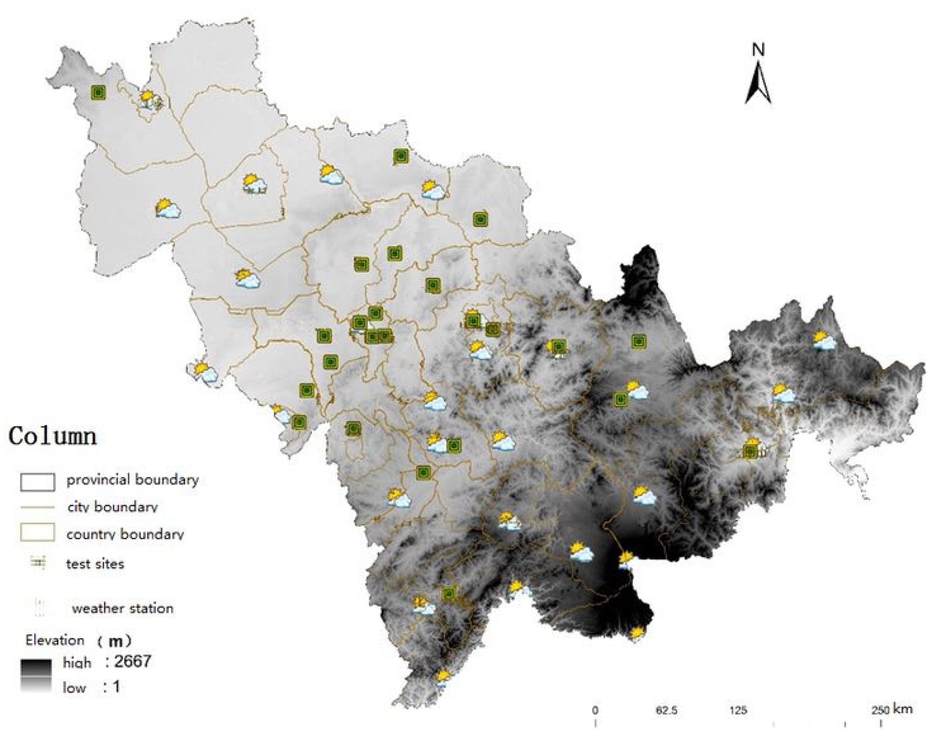
Spatial Layout of Multi-Environment Test Sites: A Case Study of Maize in Jilin Province

Abstract

Variety regional tests based on multiple environments play a critical role in understanding the high yield and adaptability of new crop varieties. However, the current approach mainly depends on experience from breeding experts and is difficulty to promote because of inconsistency between testing and actual situation. We propose a spatial layout method based on the existing systematic regional test network. First, the method of spatial clustering was used to cluster the planting environment. Then, we used spatial stratified sampling to determine the minimum number of test sites in each type of environment. Finally, combined with the factors such as the convenience of transportation and the planting area, we used spatial balance sampling to generate the layout of multi-environment test sites. We present a case study for maize in Jilin Province and show the utility of the method with an accuracy of about 94.5%. The experimental results showed that 66.7% of sites are located in the same county and the unbalanced layout of original sites is improved. Furthermore, we conclude that the set of operational technical ideas for carrying out the layout of multi-environment test sites based on crop varieties in this paper can be applied to future research.

1. Introduction

Variety regional test, as a key to new crop variety performance and market prospects, has an irreplaceable role in breeding [1]. Since 2000, United States constructed a regional test network based on hundreds of test sites to represent almost all types of planting environments [2]. China has also built a systematic regional test network [3,4,5]. To accurately assess each variety within 2–3 years, every test site must be highly representative of planting environments, which cover several elements such as weather, soil, terrain, biological factors, etc., called multi-environments. However, regional test results are still inconsistent with actual crop results. An important reason for this result is that neither the number nor the locations of test sites could adequately represent the multi-environments.

Clustering, a fundamental method in regionalization based on multi-environments, has been used in maize planting environments for different applications. To deal with the sparse data from observed stations such as meteorological data, previous studies can be divided into two major categories: (1) studies that focus on environments clustering of the site itself, for instance, ecological and climatic factors limiting maize production including drought [6,7,8], sunshine [9], insufficient accumulated temperature [10], high temperature heat damage [11], and terrain conditions [12]; and (2) studies that build index system for clustering based on transferring the observed station data mainly on calendar time into the regular grid data by spatial interpolation method [13,14,15,16,17,18]. In fact, the environmental conditions of phenophase have a greater impact on crop varieties.

The accurate prediction of new varieties would be increased by the accumulated data from the same test sites for years. Therefore, selecting suitable test sites is a prerequisite for successful testing. The factors affecting the selection of test sites are not only limit to multi-environments [19,20], but also include flat terrain, uniform fertility, good irrigation, drainage conditions, and convenient transportation [21]. Currently, the existing system mainly concerns representativeness, stability, and yield of every site. The study results from researchers whom mainly focus on the representativeness, stability, and area discrimination of every site and rarely consider the planting area [22] are difficult to apply.

Planting environmental factors, as the geographical objects, usually have a certain spatial correlation. The traditional sampling methods could not apply to planting environment. Spatial sampling algorithms that are very popular [23,24,25] are seldom used in test site layout. In some previous practical applications [26,27,28,29], sites were selected based on expert knowledge. However, as the theoretical research continues to deepen in the fields of spatial sampling algorithms and spatial autocorrelation algorithms, researchers began to use spatial sampling models to optimize the sampling results to ensure the accuracy and avoid the bias caused by the subjective judgment.

In this paper, we propose a three-stage spatial layout method: (1) based on meteorological data, soil nutrient data, and topographical data during the phenophase period, we clustered the planting environment by spatial clustering method; (2) we used spatial stratified sampling to determine the minimum number of test sites in each type of environment; and (3) combined with factors such as the convenience of transportation and the planting area, the layout of multi-environment test sites was constructed according to spatially balanced sampling method. We take maize in Jilin Province, one of the main maize producing areas, as a case study.The experimental results were compared with existing sites to verify the availability of our method.

2. Materials and Methods

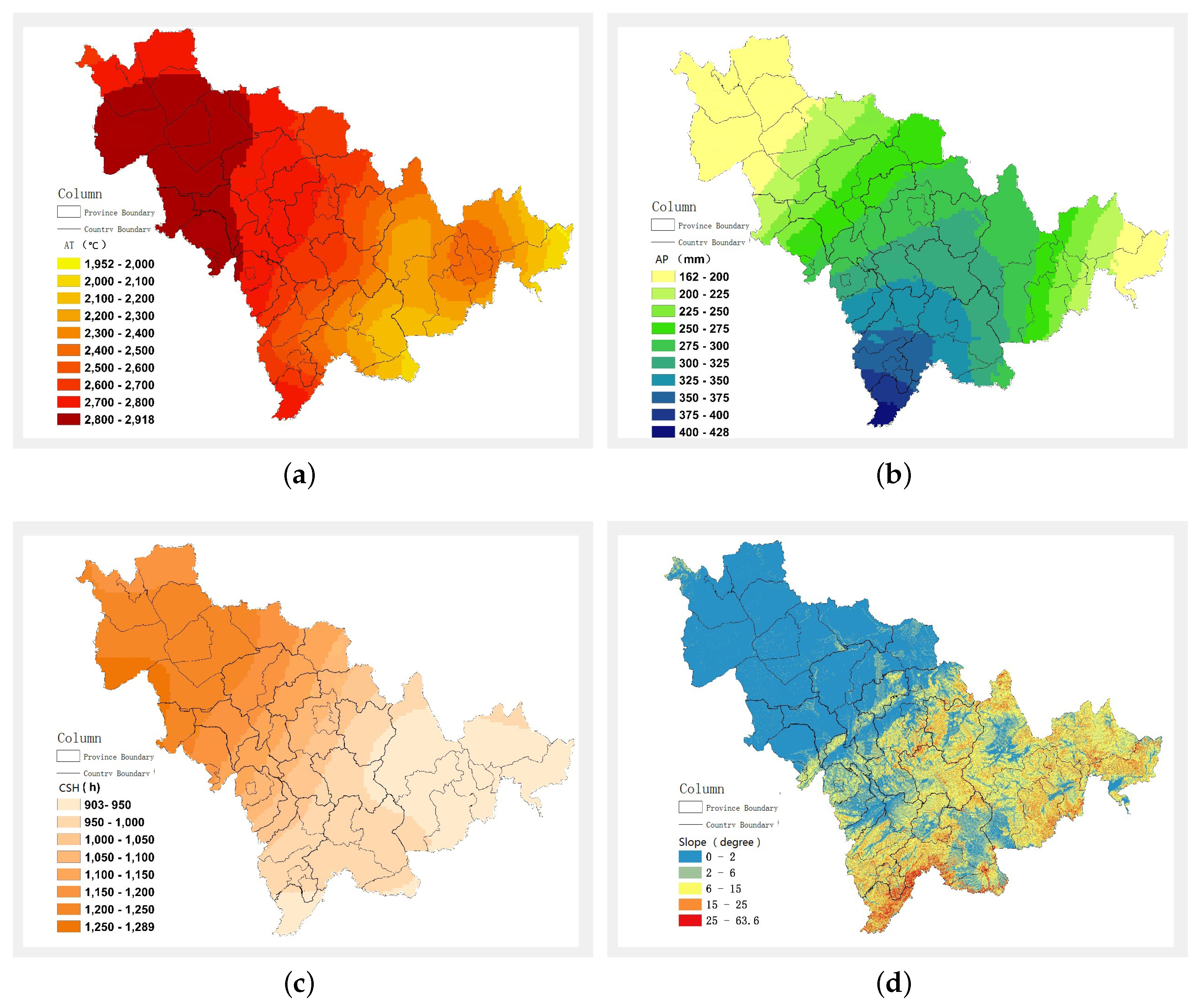
2.1. Index System Construction

The selection of indicators is the fundamental step for environmental recognition. In this paper, we use indicators as a theoretical basis for the layout of maize variety regional test sites which are used to select new varieties that are not only suitable for planting in different environments but also stable and high yield. The first principle of selecting indicators is the ecological factors that have a great impact on maize production but are independent from each other. The limiting factors of maize production mainly include cultivation and planting techniques, ecological and climatic factors, seed variety, soil, and biological stress [30]. Here, we use the following four ecological and climatic factors to build the indicator system: let {n,i} denote the days and index in grown period.

• Accumulated temperature (AT) which refers to the accumulation daily average temperature (t) from sowing to maturity is formulated as:

  $$AT=\sum _{i=1}^n{t}_{i}subjectto:t_i\ge 10{}^{\circ }\mathrm{C}$$

  (1)
• Accumulated Precipitation (AP) which refers to accumulation of precipitation during whole grown period is formulated as:

  $$AP=\sum _i^n{P}_i$$

  (2)

  $P_i$ refers to daily i precipitation (units:mm)
• Cumulative Sunshine Hours (CSH) which refers to accumulation of sunshine hours during whole grown period is formulated as:

  $$CSH=\sum _i^n{S}_i$$

  (3)
• Elevation and Slope

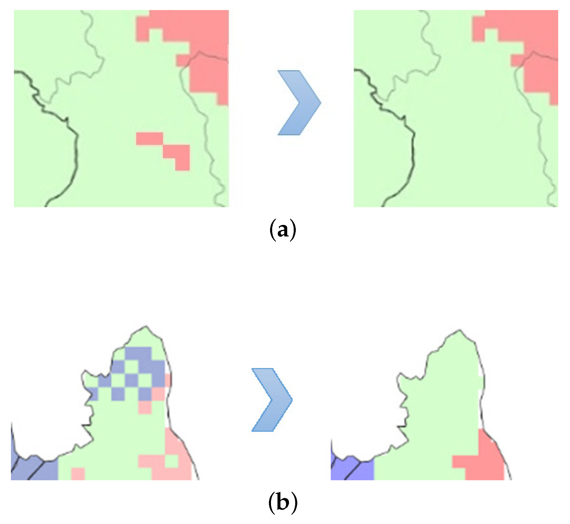
2.2. Data Pre-Processing

In this study, meteorological data were provided by National Meteorological Center of China. The phenological data of spring maize and summer maize were obtained from China crop growthand farmland soil moisture data were provided by the National Meteorological Information Center of China and the China Ministry of Agriculture. Meanwhile, we collected some survey data from Agro-Seed Industry Companies. The national geography data used in this study were 1:4 million scale provincial and county administrative division vector data. The slope data came from the DRM (Shuttle Radar Topography Mission) 90 m resolution DEM data [31]. The distribution of test sites and weather stations in Jilin Province [32] is shown in Figure 1.

We used the Global Moaran’s I index and Z points to measure the spatial autocorrelation of each indicators. Positive and negative Maran’s I index values represent the corresponding positive and negative correlations of indicators. If Z points > 1.96, the spatial object is aggregated. If Z points < −1.96, the spatial object is decentralized [33]. We used the normal QQ plot to see if the data are normally distributed, and normalized the data using Equation (4).

$$Z=\frac{x-min(X)}{max(X)-min(X)}$$

(4)

where Z denotes the normalized value of each pixel (x), and $min(X)$ and $max(X)$ denote the minimum and maximum values of all pixels (X) before normalization, respectively.

2.3. Spatial Clustering

We proposed an integrated clustering algorithm for spatial attributes based on ISOData method [34,35], where the implementation is in three phases. (1) Cluster pedigree maps: $R^2$ and semi-$R^2$, are used to evaluate the clustering results and determine the number of clusters. (2) ISOData clustering algorithm is used for the planting environment. (3) Spatial continuity adjustments are made according to spatial adjustment rules. Partitions obtained have as many differences between classes as possible, small intraclass differences, and spatial continuity.

Four criteria for determining the number of clusters based on pedigree maps are as follows: (1) The distance between the centres of gravity are as far as possible. (2) The number of classes must meet practical purposes. (3) Practical purposes lead to the number of clusters. (4) The results obtained by different clustering methods should have the same class. Assume that sample size of n is divided into k categories, as $C_1,C_2,\dots ,C_k$. $n_t$ denotes the number of samples in Class $C_t$. Let {${\dot{X}}^t$, $X_i^t$} denote the center of gravity and the i-th (i = $1,\dots ,n_t$) sample of $C_t$. $R_k^2$ is defined as follows:

$$R_k^2=1-\frac{{\sum }_{t=1}^k{W}_t}{T}$$

(5)

where $W_t={\sum }_{t=1}^{n_t}{(X_i^t-\dot{X^t})}^2$ and $T={\sum }_{t=1}^k{\sum }_{i=1}^{n_t}{(X_i^t-\dot{X^t})}^2$. We use $R_k^2$ to evaluate the performance of the clustering with k clusters.The larger $R_k^2$, the better performance based on k clusters. We also choose the semi-$R^2$ in this paper:

$$\text{semi-}{R}_k^2=R_{k+1}^2-R_k^2$$

(6)

A larger semi-$R_k^2$ means a better performance of K+1 clusters.

Two spatial data adjustment rules for the raster data are defined as follows. Scenario 1: Other clusters distribute sporadic in a certain cluster. We use area threshold to determine whether the sporadic areas are retained. Scenario 2: the areas neighbor multiple clusters. Here, we calculate the difference between this area and all neighboring clusters and merge with the nearest one. The difference value D is defined as:

$$D=\sqrt{\frac{{\sum }_{i=1}^n{({\dot{X}}_i-{\dot{Y}}_i)}^2}{n}}$$

(7)

where ${\dot{X}}_i$ denotes the mean of the i-th attribute of class of this area and ${\dot{Y}}_i$ denotes one of the near cluster. n is number of attributes of one class.

2.4. Sample Strategy

We used a spatial sampling model proposed by Zhao et al. [32]; in this study, the relationship between the number of test sites x and sampling accuracy is defined as:

$$x=\frac{(\sum W_h{S}_h\sqrt{C_k})\sum (\frac{W_h{S}_h}{\sqrt{c_h}})}{y+\frac{1}{n}\sum W_h{S}_h^2}$$

(8)

The number of samples in each layer is calculated as the following formula:

$$n_h=\frac{W_h{S}_h/\sqrt{C_h}}{\sum W_h{S}_h/\sqrt{C_h}}\times n$$

(9)

where N is the total number of grid samples, n is the number of test sites, h is the planting environment class, $N_h$ is the number of samples in the h type of planting environments, $W_h=\frac{N_h}{N}$ is the weight of h type of planting environments, $S_h$ is true standard deviation of the h type of planting environments, and $C_h$ is the cost of investigating a single sample of a planting environment.

3. Results

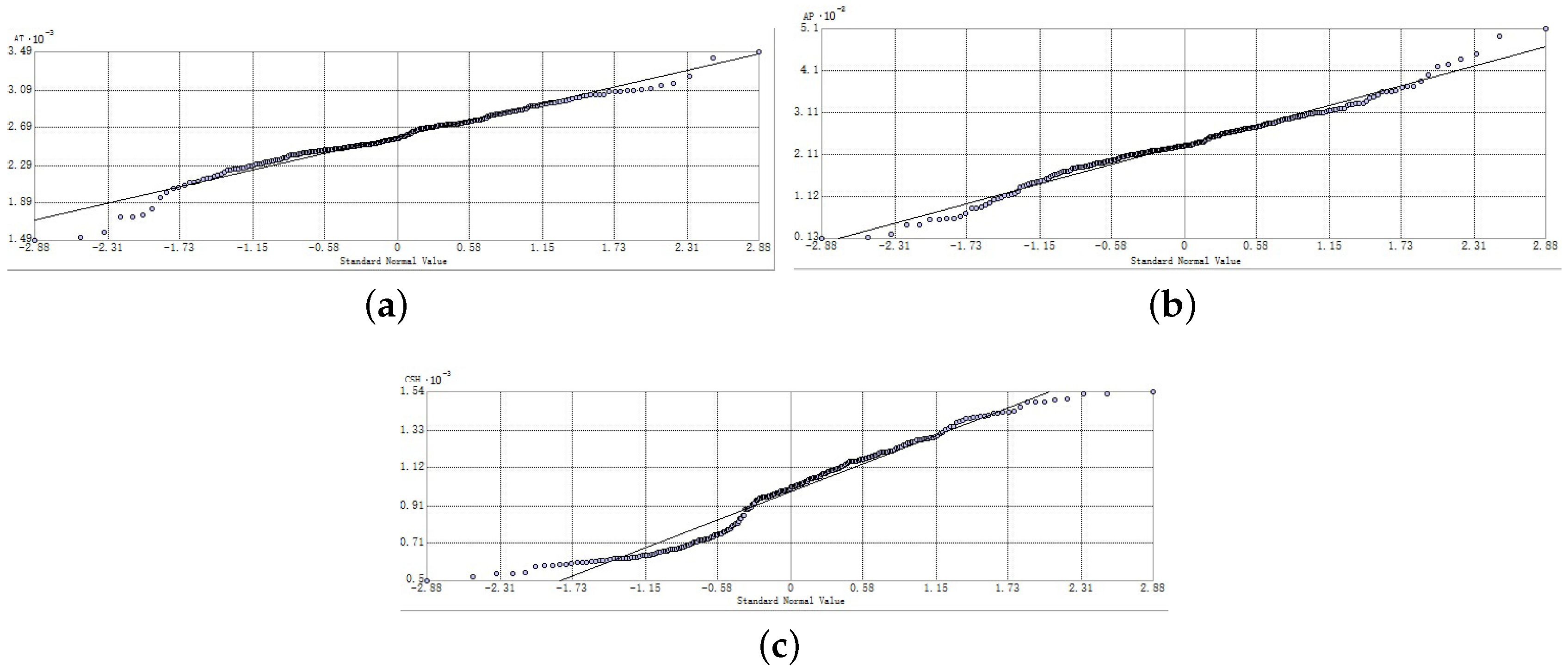
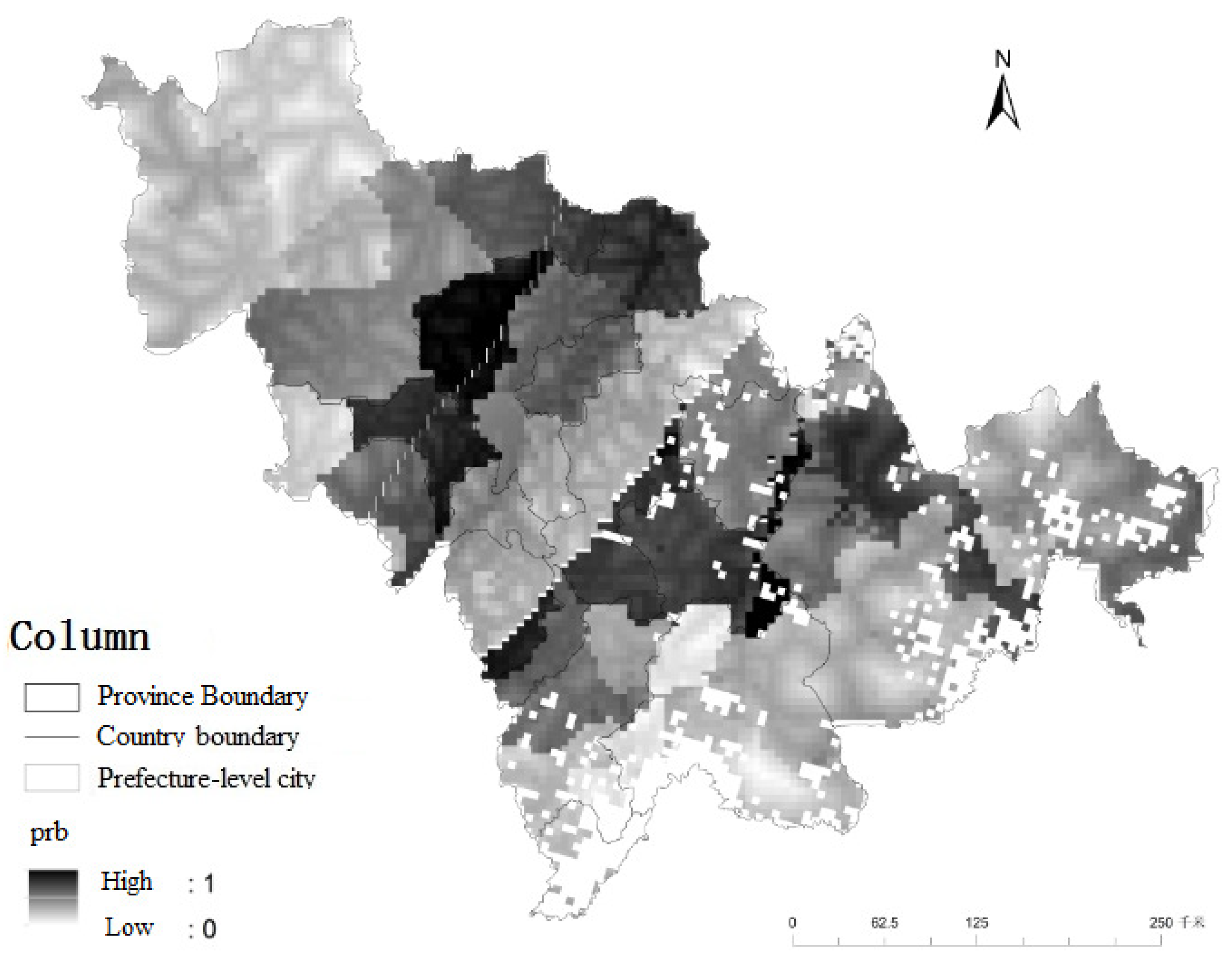
3.1. Data Processing

Moran’s I index of all three indicators is positive, which means all of them have spatial autocorrelation. The Z points are all greater than 1.96, indicating that the spatial distributions of the factors are clustered and the reliability is high (

Table 1. The Moran’s I index, Variance, and Z points of the three indicators.

Indicators	Moran I	Variance	Z points
AT	0.531548	0.006411	6.951109
AP	0.656345	0.006324	8.567889
CSH	0.685310	0.006488	8.818582

). Hence, we use statistical spatial interpolation for all three indicators.

It can be seen in Figure 2 that all three factors are close to the normal distribution and the mathematical exceptions are unknown. Thus, we used the Ordinary Kriging method to interpolate AP and CSH. As the temperature is reduced by 0.6 ${}^{\circ }$C for each 1000 m increased in elevation, we used Cokriging method to consider elevation for AT. The normal transformation parameters were not set and the grid resolution is 5000 m (Figure 3).

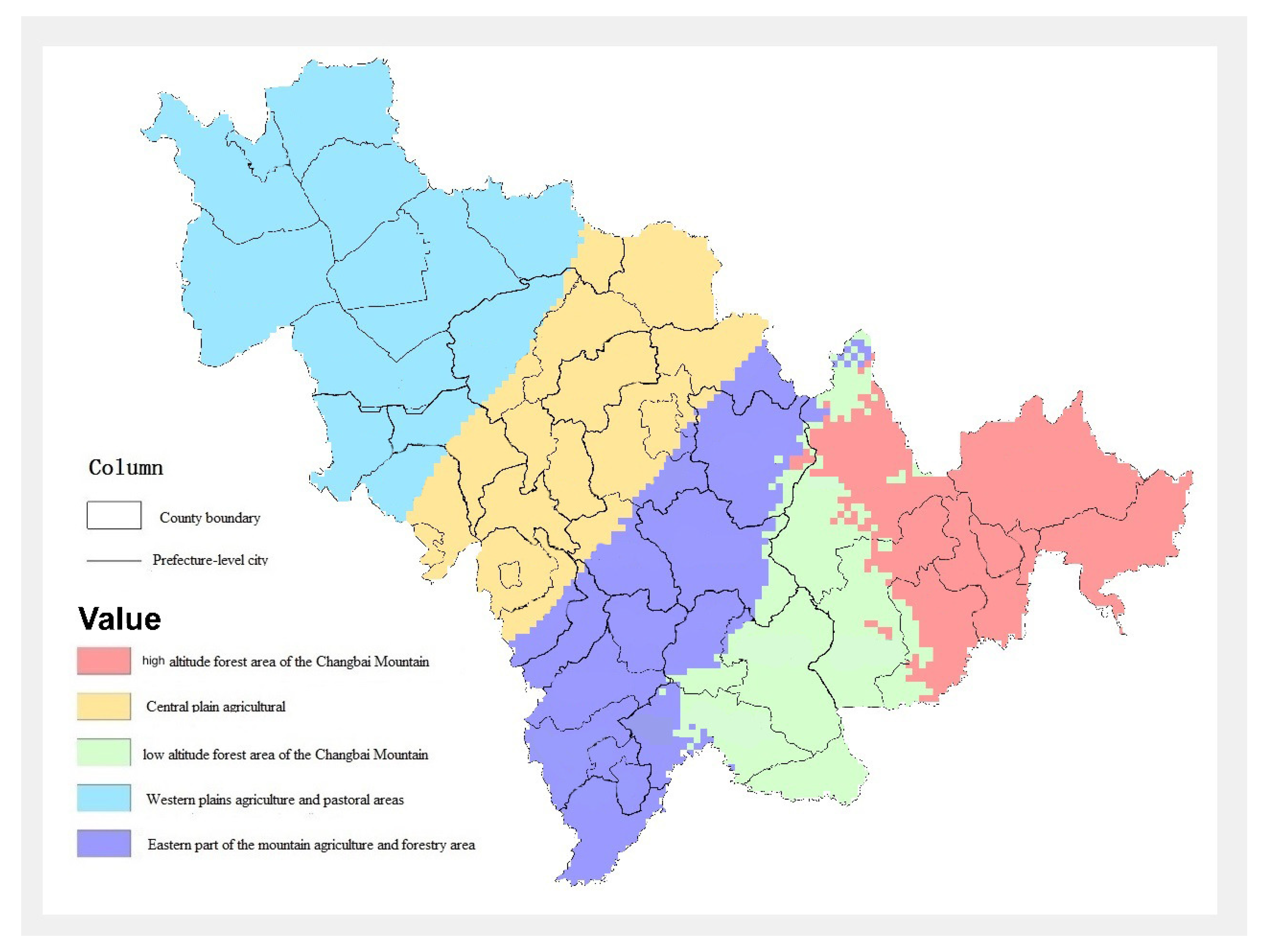
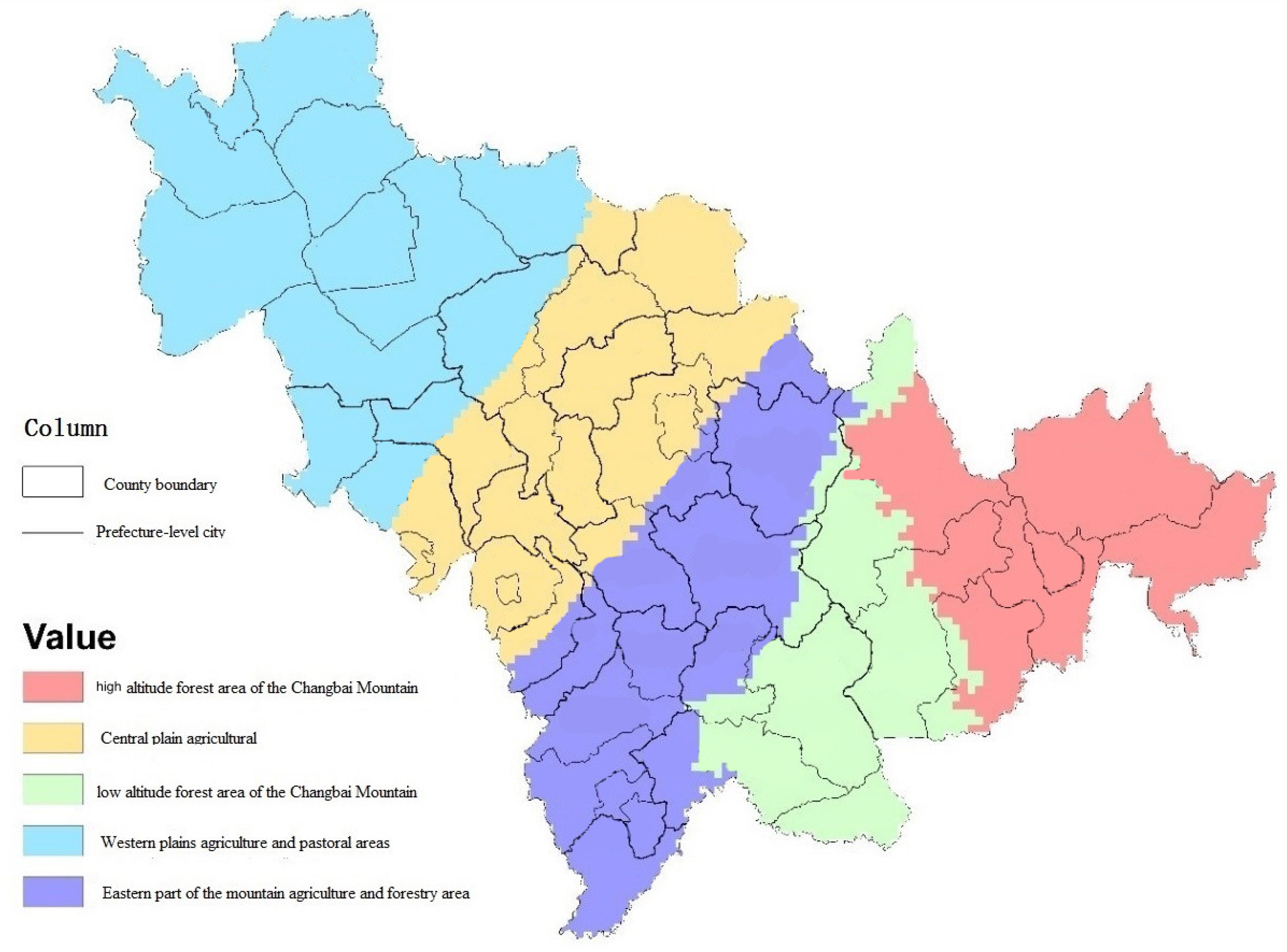
3.2. Multi-Environments Clustering

We divided the planting environments into 2–9 categories, and calculated the $R^2$ to evaluate the effect of clustering. The $R^2$ and semi-$R^2$ for different numbers of classes are shown in

Table 2. $R^2$ and semi-$R^2$ for different numbers of clusters.

Number of Clusters	${\mathit{R}}^2$	semi-${\mathit{R}}^2$
9	0.926
8	0.911	0.015
7	0.904	0.007
6	0.891	0.013
5	0.880	0.009
4	0.826	0.054
3	0.787	0.039
2	0.663	0.124

.

We found $R^2$ are all around 0.9 with no significant difference using more than five clusters. Furthermore, it is largest at four clusters, thus we selected five as the number of clusters to divide the planting environments (Figure 4).

We used spatial continuity adjustment rules in the planting environment of Jilin Province as a case study. Two methods are used to adjust planting environment (Figure 5).

Maize planting environmental divisions is shown in Figure 6.

As a result, combining geography and actual conditions, the planting environment in Jilin Province is divided into five districts: High Altitude Forest area of the Changbai Mountain (HAFCM), Low Altitude Forest area of the Changbai Mountain (LAFCM), Eastern part of the mountain Agriculture and Forestry Area (EAF), Central Plains Agricultural (CPA), and Western plain Agricultural and Pastoral Area (WAP).

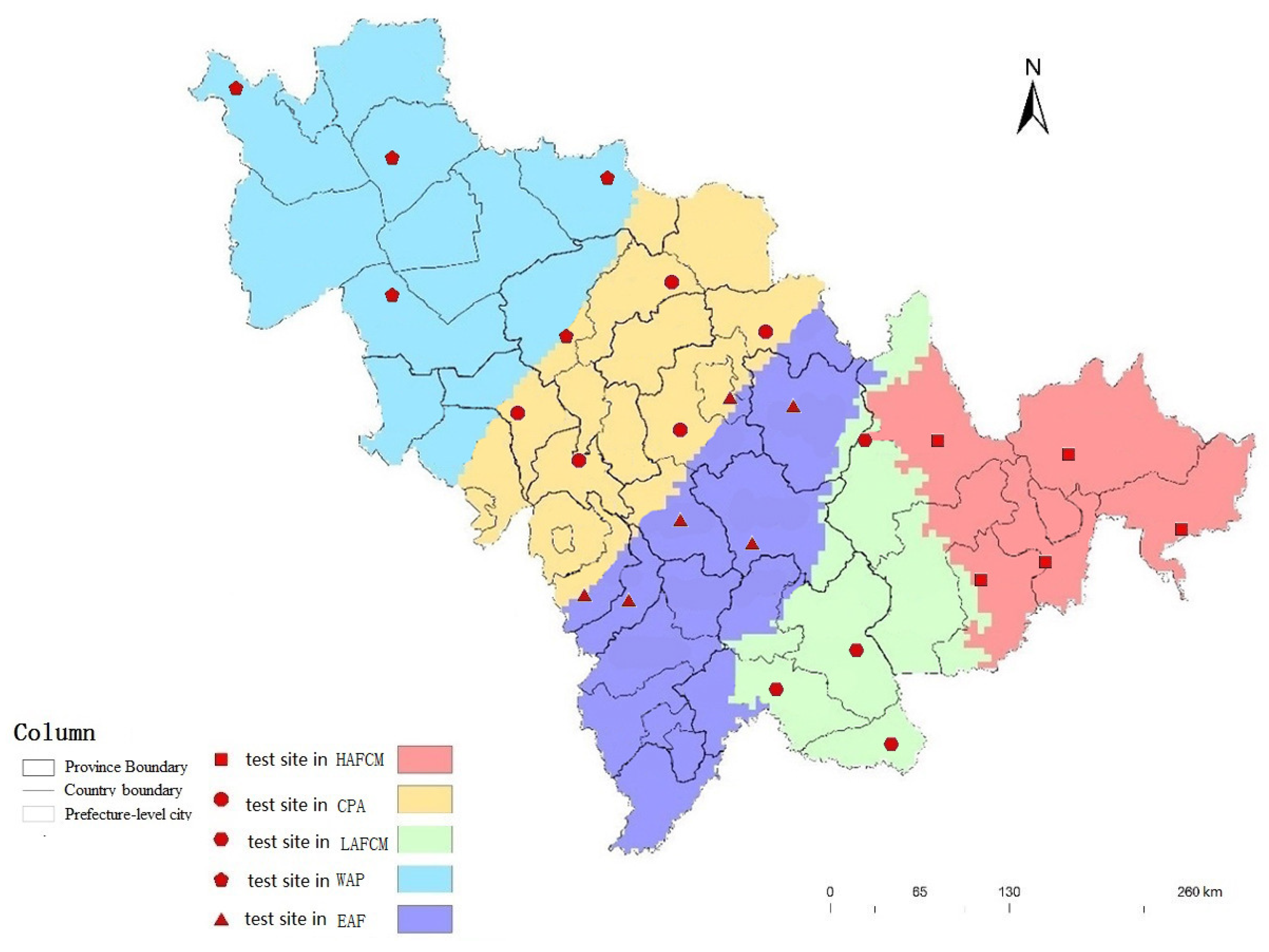
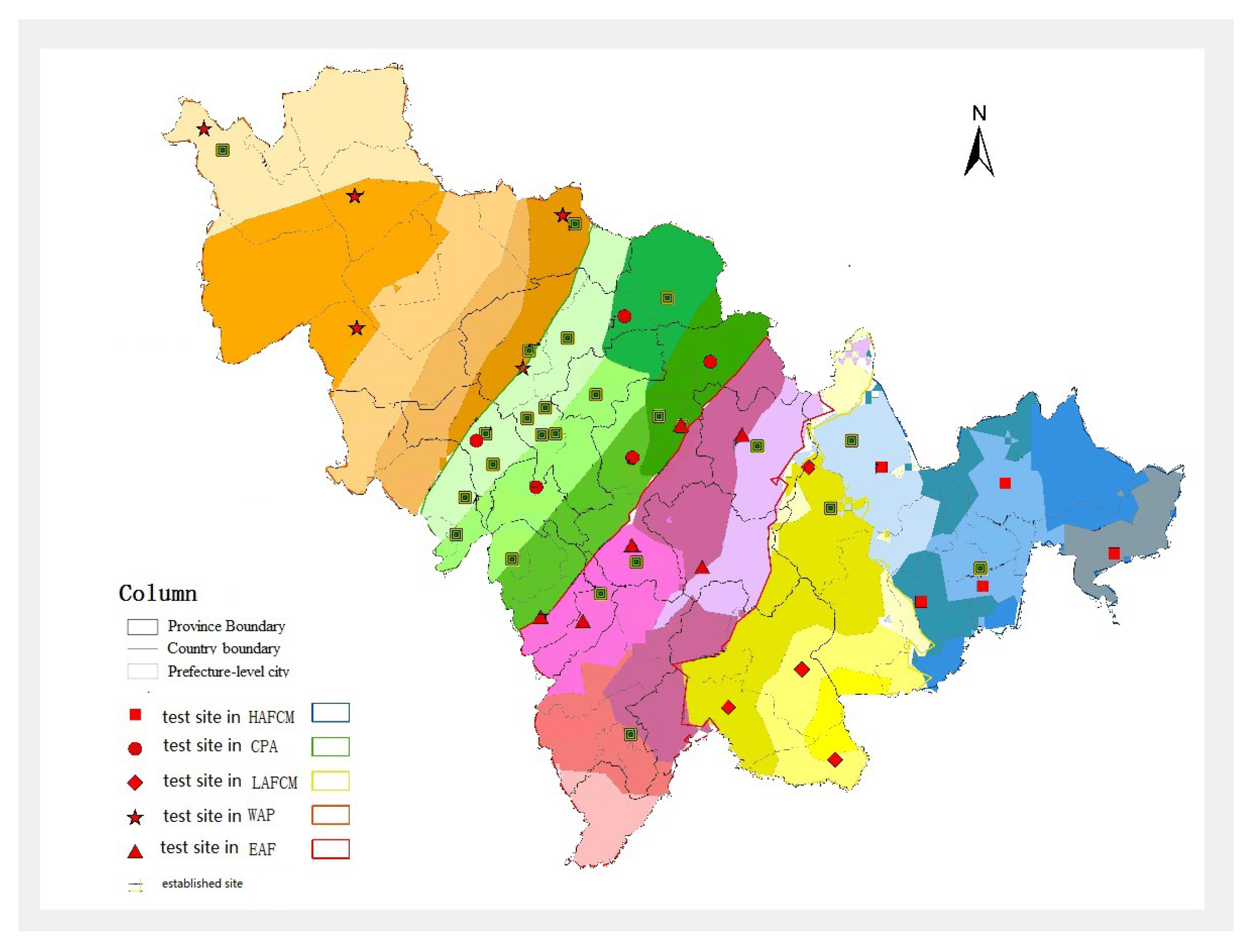
3.3. Test Sites Layout

The layout of test sites based on multi-environments in Jilin Province mainly considers the following three issues: (1) the minimum number of test sites; (2) the number of sites for each type of planting environment; and (3) the site locations. Test sites layout consists of four steps:

Step 1. In Jilin Province, in addition to the site’s ability to fully represent the different regional planting environment, the following factors should be considered: the distance to roads, and the total planted area. We use the national and provincial road data to calculate the degree of convenience for traffic.

Step 2. Using Equation (8), we can conclude that at least 25 sites should be deployed to meet the sampling accuracy requirements (error = 0.05). In this study, we also considered that the cost of single-sample surveys of all types is equal. According to Equation (9), we obtained the number of each type: $N_{(HAFCM)}=5, N_{(CPA)}=5, N_{(LAFCM)}=4, N_{(WAP)}=5, and N_{(EAF)}=6$.

Step 3. A probability grid, which was used for site location, was constructed (Figure 7) based on following three factors: (1) representation of the planting environment (pdist): the distance from the sample to the cluster center; (2) planting area (area); and (3) road distance (roaddist). Based on the expert knowledge, the weights of pdist, area, and roaddist in Jilin Province were set to: as $w_{(pdist)}=0.1,w_{(area)}=0.8,$ and $w_{(roaddist)}=0.1$. The calculation formula for the probability raster (prb) is:

$$prb=(\frac{pdist}{max(pdis)}\times w_{(pdist)}+\frac{area}{max(area)}\times w_{(area)}+[1-\frac{roaddist}{max(roaddist)}]\times w_{(roaddist)})\times slope$$

(10)

Step 4. We used spatially balanced sampling to set up a testing site for each type of planting environment. (Figure 8)

The sample relative accuracy calculated using Equation (8) is 94.5% when the number of test sites $x=25$.

4. Discussion

4.1. Clustering Attribute Statistics

The statistics of five types of planting environment are shown in

Table 3. Statistics of five types of planting environment.

Type	Range AT	Mean	Range AP	Mean	Range CSH	Mean	Range Elevation	Mean
LAFCM	1950–2500	2300	180–300	240	900–970	926	2–1481	600
HAFCM	2040–2500	2250	250–360	300	900–1000	953	330–2670	860
EAF	2330–2770	2570	280–430	340	920–1050	980	90–1500	500
CPA	2600–2900	2740	240–330	280	1030–1180	1110	130–850	240
WAP	2630–2920	2830	160–260	200	1170–1280	1217	100–640	160

.

In HAFCM, the terrain fluctuated greatly, area of maize is less, and it is prone to frost damage because of the earlier frost period. In contract, AP and CSH of LAFCM are relatively small. EAF, a semi-mountainous valley, is generally basin and plain, where the arable land is relatively large and suitable for agricultural development. The climate of this area is mild, e.g., AT is between 2330 ${}^{\circ }$C and 2770 ${}^{\circ }$C with abundant AP. CPA is the main maize belt in Jilin Province. Most of the cultivated land is concentrated and contiguous, which is suitable for mechanized farming. It has abundant photothermal resources, for instance, AT is between 2600 ${}^{\circ }$C and 2900 ${}^{\circ }$C and AP is between 240 m and 330 mm.

4.2. Planting Environmental Representation

We clustered each type of planting environment using the same clustering method, and compared them with the test site layout results.

Test sites proposed in this paper cover 19 of 25 sub-clusters (Figure 9). However, the number of test sites is still unbalanced.Two reasons may cause this situation: (1) the randomness of spatially-balanced sampling; and (2) the planting areas in sub-clusters are too small.

4.3. Comparison Number of Test Sites

The number of original test sites in Jilin province is 26 (

Table 4. Number of test sites.

Type	Established Sites	Our Method
HAFCM	2	5
LAFCM	1	4
EAF	4	6
CPA	13	5
WAP	3	5

). The spatial distribution of the existing test sites is not well-balanced. For example, in CPA, the number of test sites is 13 which is about half of the total sites. The total established test sites number of HAFCM and LAFCM cannot reflect actual complexity, comparing with nine test sites from our method. In addition, EAF and WAP also need to add two sites according to our method.

5. Conclusions

To tackle with the problems of spare data from multi-environments and inconsistence between regional tests and actual promotion, we propose a spatial layout method that includes the following two novel features: (1) It constructs a clustering index system of planting environment with test site layout as the application purpose. (2) It deduces the appropriate spatial distribution of test points in different cluster by integrating the complexity of each planting environment type. The experiment was run in Jilin Province to simulate the layout of maize variety testing sites. The results show the proposed methods can not only meet requirements for quantity measurement and spatial distribution of test sites, but also provides a set of operational technical ideas for the layout of multi-environment test sites for crop varieties.

References

1. Cooper, M.; Messina, C.D.; Podlich, D.; Totir, L.R.; Baumgarten, A.; Hausmann, N.J.; Wright, D.; Graham, G. Predicting the future of plant breeding: Complementing empirical evaluation with genetic prediction. Crop Pasture Sci. 2014, 65, 311–336. [Google Scholar] [CrossRef]
2. Burnham, L.; King, B.H.; Deline, C.; Barkaszi, S.; Sahm, A.; Stein, J. The US DOE Regional Test Center Program: Driving Innovation Quality and Reliability; Technical Report; Sandia National Laboratories (SNL-NM): Albuquerque, NM, USA, 2015.
3. Gale, F.; Jewison, M.; Hansen, J. Prospects for China’s corn yield growth and imports. Curr. Politics Econ. North. West. Asia 2016, 25, 479–521. [Google Scholar]
4. Fufeng, Q.; Jun, Y.; Torres, D.A.P. Comparison of Corn Production Costs in China, the US and Brazil and Its Implications. Agric. Sci. Technol. 2016, 17, 731–736. [Google Scholar]
5. Li, J.; Zhang, X.; Sun, S.; Wang, S. Analysis of maize variety in national maize main production area using SSR technique I. evaluation of distinctness and uniformity of maize variety. Yumi Kexue (J. Maize Sci.) 2006, 14, 3842. [Google Scholar]
6. Beyene, Y.; Semagn, K.; Crossa, J.; Mugo, S.; Atlin, G.N.; Tarekegne, A.; Meisel, B.; Sehabiague, P.; Vivek, B.S.; Oikeh, S.; et al. Improving maize grain yield under drought stress and non-stress environments in sub-Saharan Africa using marker-assisted recurrent selection. Crop Sci. 2016, 56, 344–353. [Google Scholar] [CrossRef]
7. Harrison, M.T.; Tardieu, F.; Dong, Z.; Messina, C.D.; Hammer, G.L. Characterizing drought stress and trait influence on maize yield under current and future conditions. Glob. Chang. Biol. 2014, 20, 867–878. [Google Scholar] [CrossRef] [PubMed]
8. Naveed, M.; Mitter, B.; Reichenauer, T.G.; Wieczorek, K.; Sessitsch, A. Increased drought stress resilience of maize through endophytic colonization by Burkholderia phytofirmans PsJN and Enterobacter sp. FD17. Environ. Exp. Bot. 2014, 97, 30–39. [Google Scholar] [CrossRef]
9. Zhao, J.; Guo, J.; Mu, J. Exploring the relationships between climatic variables and climate-induced yield of spring maize in Northeast China. Agric. Ecosyst. Environ. 2015, 207, 79–90. [Google Scholar] [CrossRef]
10. Meng, Q.; Hou, P.; Lobell, D.B.; Wang, H.; Cui, Z.; Zhang, F.; Chen, X. The benefits of recent warming for maize production in high latitude China. Clim. Chang. 2014, 122, 341–349. [Google Scholar] [CrossRef]
11. Lobell, D.B.; Hammer, G.L.; Chenu, K.; Zheng, B.; McLean, G.; Chapman, S.C. The shifting influence of drought and heat stress for crops in northeast Australia. Glob. Chang. Biol. 2015, 21, 4115–4127. [Google Scholar] [CrossRef] [PubMed]
12. Deb, P.; Shrestha, S.; Babel, M.S. Forecasting climate change impacts and evaluation of adaptation options for maize cropping in the hilly terrain of Himalayas: Sikkim, India. Theor. Appl. Climatol. 2015, 121, 649–667. [Google Scholar] [CrossRef]
13. Yu, W.; Chen, H. Study on precise comprehensive agricultural climate regional planning of summer maize in Henan Province. Meteorol. Environ. Sci. 2010, 33, 14–19. [Google Scholar]
14. Gong, L.; Wang, C.; Wang, P.; Lv, S.; Wang, J.; Dai, S. Variation of climate suitability of maize in the Northeast of China. J. Maize Sci. 2013, 21, 140–146. [Google Scholar]
15. Wang, D.; Li, G.; Mo, Y.; Cai, M.; Bian, X. Effect of Planting Date on Accumulated Temperature and Maize Growth under Mulched Drip Irrigation in a Middle-Latitude Area with Frequent Chilling Injury. Sustainability 2017, 9, 1500. [Google Scholar] [CrossRef]
16. Dai, L.; Li, C.; Wei, R. Climatic suitability of summer corn and its changes in Hebei province. Ecol. Environ. Sci. 2011, 20, 1031–1036. [Google Scholar]
17. Wang, L.; Xiong, W.; Wen, X.; Feng, L. Effect of climatic factors such as temperature, precipitation on maize production in China. Trans. Chin. Soc. Agric. Eng. 2014, 30, 138–146. [Google Scholar]
18. Zhao, Z.; Qu, Y.; Liu, Z.; Wu, R.; Xia, Y.; Li, S.; Zhang, X. Spatial distribution of interaction effect between variety and environment on maize yield. Trans. Chin. Soc. Agric. Eng. 2015, 31, 232–238. [Google Scholar]
19. Cooper, M.; Smith, O.; Merrill, R.; Arthur, L.; Podlich, D.; Löffler, C. Integrating breeding tools to generate information for efficient breeding: Past, present, and future. In Plant Breeding: The Arnel R. Hallauer International Symposium; Wiley Online Library, 2008; pp. 141–154. [Google Scholar]
20. Crosbie, T.M.; Eathington, S.R.; Johnson, G.R.; Edwards, M.; Reiter, R.; Stark, S.; Mohanty, R.G.; Oyervides, M.; Buehler, R.E.; Walker, A.K.; et al. Plant breeding: Past, present, and future. In Plant Breeding: The Arnel R. Hallauer International Symposium; Wiley Online Library: Hoboken, NJ, USA, 2006; pp. 3–50. [Google Scholar]
21. Butruille, D.V.; Birru, F.H.; Boerboom, M.L.; Cargill, E.J.; Davis, D.A.; Dhungana, P.; Dill, G.M.; Dong, F.; Fonseca, A.E.; Gardunia, B.W.; et al. Maize breeding in the United States: Views from within Monsanto. Plant Breed. Rev. 2015, 39, 199–282. [Google Scholar]
22. Liu, Z.; Yang, J.; Li, S.; Wang, H.; Li, L.; Zhang, X.; Zhu, D. Optimal method of transforming observables into relative values for multi-environment trials in maize. Trans. Chin. Soc. Agric. Eng. 2011, 27, 205–209. [Google Scholar]
23. Delmelle, E. Optimization of Second-Phase Spatial Sampling Using Auxiliary Information. Ph.D. Thesis, The State University of New York, Buffalo, NY, USA, 2005. [Google Scholar]
24. Fischer, M.M.; Wang, J. Spatial Data Analysis: Models, Methods and Techniques; Springer Science & Business Media: Luxemburg, Germany, 2011. [Google Scholar]
25. Wang, J.F.; Stein, A.; Gao, B.B.; Ge, Y. A review of spatial sampling. Spat. Stat. 2012, 2, 1–14. [Google Scholar] [CrossRef]
26. Liu, T.; Wang, J.; Xu, C.; Ma, J.; Zhang, H.; Xu, C. Sandwich mapping of rodent density in Jilin Province, China. J. Geogr. Sci. 2018, 28, 445–458. [Google Scholar] [CrossRef]
27. Wang, J.F.; Jiang, C.S.; Hu, M.G.; Cao, Z.D.; Guo, Y.S.; Li, L.F.; Liu, T.J.; Meng, B. Design-based spatial sampling: Theory and implementation. Environ. Model. Softw. 2013, 40, 280–288. [Google Scholar] [CrossRef]
28. Grafström, A.; Lundström, N.L.; Schelin, L. Spatially balanced sampling through the pivotal method. Biometrics 2012, 68, 514–520. [Google Scholar] [CrossRef] [PubMed]
29. Wang, J.F.; Zhang, T.L.; Fu, B.J. A measure of spatial stratified heterogeneity. Ecol. Indic. 2016, 67, 250–256. [Google Scholar] [CrossRef]
30. Hou, P.; Liu, Y.; Xie, R.; Ming, B.; Ma, D.; Li, S.; Mei, X. Temporal and spatial variation in accumulated temperature requirements of maize. Field Crops Res. 2014, 158, 55–64. [Google Scholar] [CrossRef]
31. Liu, Z.; Qu, Y.; Zhao, Z.; Li, S.; Zhang, X. Temporal and spatial law of promotion center moving and diffusion of excellent maize varieties. Trans. Chin. Soc. Agric. Eng. 2018, 34, 178–185. [Google Scholar]
32. Zhao, Z.; Zhang, X.; Liu, Z.; Yao, X.; Li, S.; Zhu, D. Spatial sampling of multi-environment trials data for station layout of maize variety. In Proceedings of the 2017 6th International Conference on Agro-Geoinformatics, Agro-Geoinformatics, Fairfax, VA, USA, 7–10 August 2017; pp. 1–6. [Google Scholar]
33. Bezdek, J.C. A convergence theorem for the fuzzy ISODATA clustering algorithms. IEEE Trans. Pattern Anal. Mach. Intell. 1980, PAMI-2, 1–8. [Google Scholar] [CrossRef]
34. Abbas, A.W.; Minallh, N.; Ahmad, N.; Abid, S.A.R.; Khan, M.A.A. K-Means and ISODATA Clustering Algorithms for Landcover Classification Using Remote Sensing. Sindh Univ. Res. J.-SURJ (Sci. Ser.) 2016, 48, 315–318. [Google Scholar]
35. Chen, Z.; Chen, Y.; Hu, L.; Wang, S.; Jiang, X.; Ma, X.; Lane, N.D.; Campbell, A.T. ContextSense: Unobtrusive discovery of incremental social context using dynamic bluetooth data. In Proceedings of the 2014 ACM International Joint Conference on Pervasive and Ubiquitous Computing: Adjunct Publication, Seattle, WA, USA, 13–17 September 2014; pp. 23–26. [Google Scholar]
Figure 1. Test sites and weather stations in Jilin Province.
Sustainability 10 01424 g001
Figure 2. The normal plots for AT, AP and CSU of the whole growing period: (a) AT; (b) AP; and (c) CSH.
Sustainability 10 01424 g002
Figure 3. Spatial Distribution of indicators: (a) AT raster by Cokriging interpolation method Considering Elevation; (b) AP raster by Ordinary Kriging method interpolation; (c) CSH raster by Ordinary Kriging method interpolation; and (d) slope of Jilin Province at 90m resolution.
Sustainability 10 01424 g003
Figure 4. Preliminary classification results.
Sustainability 10 01424 g004
Figure 5. Spatial continuity adjustment: (a) Sporadic distribution of other class (red middle) in a certain class (green background). They would be adjusted directly into the adjacent major categories. (b) A region (red upper) is adjacent to more than one class (purple upper and green background) at the same time. Thus, the two types of minimum values are classified into one. The colors filled in the grids represent the same clusters as in Figure 4.
Sustainability 10 01424 g005
Figure 6. Maize planting environmental divisions.
Sustainability 10 01424 g006
Figure 7. Probability grid. The colors represent probability calculated by Equation (10).
Sustainability 10 01424 g007
Figure 8. Layout of test sites.
Sustainability 10 01424 g008
Figure 9. Map of sub-clusters. Different color levels of each cluster represent the sub-clusters in each cluster.
Sustainability 10 01424 g009