Toward the Coordinated Sustainable Development of Urban Water Resource Use and Economic Growth: An Empirical Analysis of Tianjin City, China

Abstract

The coordinated sustainable development of urban water resources and economic growth requires a better understanding of the relationship between industrial water use and economic growth. This study analyzed the relationship between urban industrial water use and economic development in Tianjin City in China (one of the four municipalities directly under the Central Government) from 2005 to 2015. The research combined the logarithmic mean Divisia index model with the Tapio model to develop a new decoupled model analyzing the relationship between urban industrial water use and economic development. The results show that: (1) Tianjin’s industrial water use and economic growth show a clear decoupling; (2) the economic scale effect drives Tianjin’s total industrial water use and economic growth towards weaker decoupling, stabilizing in a weakly decoupled state; and (3) the industrial structure effect and industrial water intensity effect drive the decoupling of industrial water use and economic growth in Tianjin. Finally, the paper provides policy recommendations to promote the decoupling of industrial water use and economic growth.

1. Introduction

Water is an indispensable natural resource and a strategic economic resource for human survival and development. Water resources provide a material basis for the sustainable development of a social economy. China is currently experiencing a gradual deepening of its social economy development and is continuously improving its industrialization and urbanization. The makes the problem of water resource utilization and economic growth increasingly prominent. As one of six megacities in China, Tianjin’s economy has been rapidly and sustainably developing. From 2005–2015, the megacity’s gross domestic product (GDP) grew by 3.8 times, with an average annual growth rate of 14.29%. The population exceeded ten million, with an average annual growth rate of 4.02%. The total volume of water resources was 1.28 billion cubic meters in 2015, accounting for 0.05% of the total water resources in China. The per capita available water volume was only 83.6 cubic meters, which was approximately 1/24 (4%) the national average. These conditions are leading to significant conflicts in the supply and demand of water resources. Given this background, it is important to study the decoupling relationship between industrial water use and economic growth as well as the factors driving the decoupling for Tianjin. This information would help adjust relevant industry development policies, optimize water resources allocation and promote the construction of a water-saving and sustainable society.

Decoupling analyses have been widely applied in recent years. Three main analysis methods are widely used. The first method is the decoupling index model proposed by Organization for Economic Co-operation and Development (OECD) [1]. OECD quantitatively studied the relationship between economic development and water resources utilization/environmental pressure and proposed models for determining relative decoupling and absolute decoupling. The second method is comprehensive decoupling analysis based on variation [2,3]. This method is based on a decoupling relationship study analyzing GDP development and material consumption by 15 members of European Union (EU). The method divides decoupling relationship into six categories. The third method is a decoupling elasticity method, proposed by Tapio [4]. Tapio used this method to analyze the relationship between the GDP of European transportation, the volume of transportation and carbon dioxide (CO₂) emissions from 1970 to 2001. The method specifically divides the decoupling relationship into eight categories.

With the continuous development of decoupling theories and methods, there has been an increase in research on decoupling theories around the worlds [5,6,7,8,9,10,11,12]. In contrast with many previous, large-scale studies, Conrad and Cassar [6] studied the small island of Malta, decoupling economic development from environmental degradation. Environmental degradation was represented by the changes of various environmental indicators, including waste. Wei [7] quantitatively used decoupling theory to investigate the decoupling relationship between economic growth and cultivated land losses caused by the construction occupation in Beijing. Taiyang et al. [8] evaluated the decoupling relationship between GDP growth and construction land expansion across China, 31 provinces in China, non-agricultural sectors and tertiary industry respectively . This was done by constructing a decoupling model of economic growth and construction land expansion. Schandl et al. [9] decoupled environmental pressure from economic growth across thirteen major countries or regions globally from 1990 to 2010 and estimated their material consumption, energy use and carbon footprint from 2010–2050. The results showed that with appropriate policies, it is possible to simultaneously achieve the objectives of sustainable development and economic growth [10]. Naqvi and Zwickl [11] used six economic sectors and six pollution indicators to analyze the decoupling relationship between emissions and GDP growth using a consistent dataset for the EU18 countries. They then analyzed the changes in decoupling states during two sub–periods (1995–2001, 2001–2008) on a country level, applying the decoupling theory of Tapio. Decoupling theories have also been widely used to research carbon emissions and economic growth at the national level [5,12,13,14,15,16], regional level [17,18,19,20] and industrial level [21,22,23,24].

Many previous studies highlight that decoupling analysis has been widely used to decouple the relationships between economic growth and environmental degradation, cultivated land loss, environmental pressure, air pollution and carbon emissions. However, little research has been completed about the decoupling relationship between water resource utilization and economic growth. Hong-li et al. [25] studied the decoupling relationship between total water volume and GDP growth, water utilization and the added value of agriculture and water utilization and the added value of industry for Yunnan province and Guizhou province. Based on the decoupling classification of Vehmas, they further divided the decoupling relationship into six categories. In an United Nations Environment Program (UNEP) Information Resource Planning (IRP) Report, Urama et al. [26] noted the appearance of a relative decoupling of economic growth from water; however, people confronting water problems accounted for almost one-third of the global population. Moreover, problems such as water scarcity and water pollution intensified due to human activities.

Solving the water crisis requires urgent measures to promote the decoupling of water use from economic development. However, research on the decoupling relationship between water utilization and economic development has been still insufficient and deeper study is needed.

Many existing water resource researchers use the measure of water footprint. Arto, Andreoni and Rueda-Cantuche [27] estimated complete time series data from 1995 to 2008 for water use, water footprints and water trade balances for forty-one regions. The research provided useful information for scientific research and policy-setting. Miglietta, De Leo and Toma [28], using a country water footprint, investigated the Environmental Kuznets Curve (EKC) hypothesis to figure out the relationship between water usage and economic development. Miglietta, Morrone and De Leo [29], taking renewable and non-renewable sources into consideration, analyzed the production of electricity by using water footprint as well as economic water productivity approaches. Pellicer-Martínez and Martínez-Paz [30] used a water footprint indicator to assess the environmental sustainability of water resources management at the river basin level. Sallam [31] focused on water resource conflicts between Egypt and Ethiopia in the Nile River Basin and chose a water footprint indicator to study the fair use of shared water resources. However, while the logarithmic mean Divisia index (LMDI) method, without an unexplained residual term, has been extensively used to research energy consumption [5,12,24,32,33,34,35,36] and carbon emissions [5,12,37,38,39,40,41,42], it has been used less in water resource research.

Zhao and Chen [43] applied the LMDI method to decompose the agricultural water footprint of China into a diet structure effect, an efficiency effect, an economic activity effect and a population effect. They further investigated the influence of these effects on the agricultural water footprint. Zhang et al. [44] used the oasis city of Urumqi as a case study, investigating the factors influencing changes in the total volume and intensity of water utilization. Studies applying the LMDI decomposition method in the field of water resources have achieved some successes, however, the depth and breadth of studies have been greater in other domains, including energy consumption and carbon emissions. Further, few studies have combined the LMDI decomposition method and decoupling method to study the relationship between water resources utilization and economic development. Given this background, this paper decomposed the total volume of industrial water and systematically analyzed decoupling states and driving factors of industrial water utilization and economic growth in Tianjin based on the constructed water decoupling model and LMDI decomposition method.

The rest of this paper is organized as follows: Section 2 presents the constructed water decoupling model and LMDI decomposition method; Section 3 presents the empirical research for the decoupling states and describes the factors driving industrial water utilization and economic growth; and Section 4 focuses on optimizing the relationship between industrial water utilization and economic growth and proposes policy solutions that may serve as theoretical references for the construction of a water-saving and sustainable society in Tianjin.

2. Materials and Methods

2.1. Construction of Water Decoupling Model

“Decoupling” is an index used to describe the asynchronous changes of two correlated variables in a given time period. When studying the relationship between economic development and resource consumption, decoupling can be defined as the fracturing of the coupling relationship between the two. When researching the relationship between the economic development and carbon emissions of 20 European countries during 1970–2001, Tapio further proposed a decoupling elastic model

$$\mathrm{e}=\frac{\Delta {\mathrm{co}}_2/{\mathrm{co}}_2}{\Delta \mathrm{G}/\mathrm{G}}$$

(1)

(In this expression, $\Delta {\mathrm{co}}_2/{\mathrm{co}}_2$ represents the carbon emission growth rate; G represents the Gross Domestic Product (GDP); and $\Delta \mathrm{G}/\mathrm{G}$ represents the economic growth rate). It specifically describes the relationship between economic development and carbon emissions.

This study applied the Tapio decoupling elastic model to build a decoupling model focused on industrial water utilization and economic growth. This approach directly replaced carbon emission growth with economic growth rate.

$${\mathrm{e}}_{(\mathrm{H},\mathrm{G})}=\frac{\Delta \mathrm{H}/\mathrm{H}}{\Delta \mathrm{G}/\mathrm{G}}$$

(2)

In Equation (1), ${\mathrm{e}}_{(\mathrm{H},\mathrm{G})}$ represents the decoupling elasticity coefficient of the relationship between industrial water utilization and economic growth; H represents the total volume of industrial water; and $\Delta \mathrm{H}/\mathrm{H}$ represents the industrial water utilization growth rate.

In previous studies, most scholars have defined decoupling and negative decoupling using e = 1. Decoupling states have been divided into 6 categories: strong decoupling, weak decoupling, recessive decoupling, expansive negative decoupling, strong negative decoupling and weak negative decoupling. Tapio was concerned that slight changes not be over-interpreted as significant. As such, the Tapio model uses a ±20% range with the original defined value. That is, the studied value ranges from 0.8 to 1.2; this range of 0.8 < e < 1.2 is defined as the coupling range. Based on changes in the industrial water utilization and economic growth rates, coupling can be divided into two categories: expansive coupling and recessive coupling. The 8 decoupling state categories are provided in

Table 1. Classification of decoupling states.

Decoupling State		$\Delta \mathit{H}/\mathit{H}$	$\Delta \mathit{G}/\mathit{G}$	Elasticity
decoupling	Strong decoupling	<0	>0	e < 0
	Weak decoupling	>0	>0	0 < e < 0.8
	Recessive decoupling	<0	<0	e > 1.2
Negative decoupling	Expansive negative decoupling	>0	>0	e > 1.2
	Strong negative decoupling	>0	<0	e < 0
	Weak negative decoupling	<0	<0	0 < e < 0.8
coupling	Expansive coupling	>0	>0	0.8 < e < 1.2
	Recessive coupling	<0	<0	0.8 < e < 1.2

[4].

Specifically, when the industrial water utilization and economic growth synchronously increase, the states that elasticity falls in the range of 0–0.8, 0.8–1.2 and beyond 1.2 can be defined as weak decoupling, expansive coupling and expansive negative decoupling, respectively. In addition, when the industrial water utilization and economic growth synchronously decrease, the states that elasticity falls in the range of 0–0.8, 0.8–1.2 and beyond 1.2 can be defined as weak negative decoupling, recessive coupling and recessive decoupling, respectively. The rest two states are strong decoupling and strong negative decoupling.

Strong negative decoupling is the worst state. It indicates a recessive economy, while industrial water utilization is increasing. This shows that economic development is not aligned with resource consumption. Strong decoupling is the best state. It indicates that economic growth is increasing, while industrial water utilization is decreasing. The process of encouraging and guiding the relationship between industrial water utilization and economic growth towards strong decoupling can promote the construction of a water-saving society.

2.2. LMDI Decomposition Model

Generally, there are two major techniques for assessing changes: structural decomposition analysis (SDA (SDA is also called IOD (the Input- Output decomposition). It is scientific but for its dependency on Input-Output data, it is hardly used in comparison of regions and time-series analysis.)) as well as index decomposition analysis (IDA (IDA is also called INA (index number analysis).)). The use of SDA is limited for its dependency on Input-Output data. Instead, IDA is extensively used in research because it can apply time-series data and panel data easily [45].

The frequently used form of IDA mainly includes LMDI, which was proposed by Ang [46] and complete decomposition model (CDM), which was proposed by SUN [47] on the basis of the Laspeyres index method.

Due to the complete decomposition of changes in total amounts, without an unexplained residual term, the LMDI method is widely used to decompose factors that contribute to changes in total amounts of a certain measure.

Based on the LMDI decomposition method and Kaya identity [48], this study decomposed the total industrial water utilization of Tianjin as follows:

$$\mathrm{H}={\displaystyle \sum }_{\mathrm{i}}{\mathrm{H}}_{\mathrm{i}}={\displaystyle \sum }_{\mathrm{i}}\left(\frac{{\mathrm{H}}_{\mathrm{i}}}{{\mathrm{G}}_{\mathrm{i}}}·\frac{{\mathrm{G}}_{\mathrm{i}}}{\mathrm{G}}·\frac{\mathrm{G}}{\mathrm{P}}·\mathrm{P}\right)={\displaystyle \sum }_{\mathrm{i}}{(\mathrm{S}}_{\mathrm{i}}·{\mathrm{T}}_{\mathrm{i}}·\mathrm{g}·\mathrm{P})$$

(3)

In this expression, ${\mathrm{H}}_{\mathrm{i}}$ represents the total water utilization of industry; ${\mathrm{G}}_{\mathrm{i}}$ represents the added value of industry; $\mathrm{G}={\displaystyle \sum }_{\mathrm{i}}{\mathrm{G}}_{\mathrm{i}}$; p represents the population of Tianjin. Further, ${\mathrm{S}}_{\mathrm{i}}=\frac{{\mathrm{G}}_{\mathrm{i}}}{\mathrm{G}}$ represents the proportion of the added value that industry provided to Tianjin GDP. In other words, industrial structure, ${\mathrm{T}}_{\mathrm{i}}=\frac{{\mathrm{H}}_{\mathrm{i}}}{{\mathrm{G}}_{\mathrm{i}}},$ represents the water utilization for each unit of added value from industry. In other words, industrial water utilization intensity, $\mathrm{g}=\frac{\mathrm{G}}{\mathrm{P}}$ represents the per capita GDP, or, economic scale.

According to the LMDI additive decomposition method, the changes in industrial water utilization from year 0 to year t can be further rewritten as:

$$\Delta {\mathrm{H}=\mathrm{H}}^{\mathrm{t}}{-\mathrm{H}}^0{=\mathrm{S}}_{\mathrm{i}}^{\mathrm{t}}·{\mathrm{T}}_{\mathrm{i}}^{\mathrm{t}}·{\mathrm{g}}^{\mathrm{t}}·{\mathrm{P}}^{\mathrm{t}}{-\mathrm{S}}_{\mathrm{i}}^0·{\mathrm{T}}_{\mathrm{i}}^0·{\mathrm{g}}^0·{\mathrm{P}}^0=\Delta {\mathrm{H}}_{\mathrm{S}}+\Delta {\mathrm{H}}_{\mathrm{T}}+\Delta {\mathrm{H}}_{\mathrm{g}}+\Delta {\mathrm{H}}_{\mathrm{P}}$$

(4)

In this expression, $\Delta {\mathrm{H}}_{\mathrm{S}},\Delta {\mathrm{H}}_{\mathrm{T}},\Delta {\mathrm{H}}_{\mathrm{g}}\mathrm{and}\Delta {\mathrm{H}}_{\mathrm{P}}$ represent the industrial structure effect, industrial water utilization intensity effect, economic scale effect and population effect, respectively. More specific expressions follow:

$$\Delta {\mathrm{H}}_{\mathrm{S}}={\displaystyle \sum }_{\mathrm{i}}\frac{{\mathrm{H}}_{\mathrm{i}}^{\mathrm{t}}{-\mathrm{H}}_{\mathrm{i}}^0}{{\mathrm{lnH}}_{\mathrm{i}}^{\mathrm{t}}{-\mathrm{lnH}}_{\mathrm{i}}^0}\times \ln \frac{{\mathrm{S}}_{\mathrm{i}}^{\mathrm{t}}}{{\mathrm{S}}_{\mathrm{i}}^0}$$

(5)

$$\Delta {\mathrm{H}}_{\mathrm{T}}={\displaystyle \sum }_{\mathrm{i}}\frac{{\mathrm{H}}_{\mathrm{i}}^{\mathrm{t}}{-\mathrm{H}}_{\mathrm{i}}^0}{{\mathrm{lnH}}_{\mathrm{i}}^{\mathrm{t}}{-\mathrm{lnH}}_{\mathrm{i}}^0}\times \ln \frac{{\mathrm{T}}_{\mathrm{i}}^{\mathrm{t}}}{{\mathrm{T}}_{\mathrm{i}}^0}$$

(6)

$$\Delta {\mathrm{H}}_{\mathrm{g}}={\displaystyle \sum }_{\mathrm{i}}\frac{{\mathrm{H}}_{\mathrm{i}}^{\mathrm{t}}{-\mathrm{H}}_{\mathrm{i}}^0}{{\mathrm{lnH}}_{\mathrm{i}}^{\mathrm{t}}{-\mathrm{lnH}}_{\mathrm{i}}^0}\times \ln \frac{{\mathrm{g}}^{\mathrm{t}}}{{\mathrm{g}}^0}$$

(7)

$$\Delta {\mathrm{H}}_{\mathrm{P}}={\displaystyle \sum }_{\mathrm{i}}\frac{{\mathrm{H}}_{\mathrm{i}}^{\mathrm{t}}{-\mathrm{H}}_{\mathrm{i}}^0}{{\mathrm{lnH}}_{\mathrm{i}}^{\mathrm{t}}{-\mathrm{lnH}}_{\mathrm{i}}^0}\times \ln \frac{{\mathrm{P}}^{\mathrm{t}}}{{\mathrm{P}}^0}$$

(8)

2.3. Expansion of Water Decoupling Model

According to Equations (1) and (3) and based on the LMDI decomposition method, this study expanded the water decoupling model of industrial water utilization and economic growth:

$${\mathrm{e}}_{\left(\mathrm{H},\mathrm{G}\right)}=\frac{\Delta \mathrm{H}/\mathrm{H}}{\Delta \mathrm{G}/\mathrm{G}}=\frac{(\Delta {\mathrm{H}}_{\mathrm{S}}+\Delta {\mathrm{H}}_{\mathrm{T}}+\Delta {\mathrm{H}}_{\mathrm{g}}+\Delta {\mathrm{H}}_{\mathrm{P}}/\mathrm{H})}{\Delta \mathrm{G}/\mathrm{G}}=\frac{\Delta {\mathrm{H}}_{\mathrm{S}}/\mathrm{H}}{\Delta \mathrm{G}/\mathrm{G}}+\frac{\Delta {\mathrm{H}}_{\mathrm{T}}/\mathrm{H}}{\Delta \mathrm{G}/\mathrm{G}}+\frac{\Delta {\mathrm{H}}_{\mathrm{g}}/\mathrm{H}}{\Delta \mathrm{G}/\mathrm{G}}+\frac{\Delta {\mathrm{H}}_{\mathrm{P}}/\mathrm{H}}{\Delta \mathrm{G}/\mathrm{G}}$$

(9)

The decoupling elasticity of Tianjin industrial water utilization and economic growth can be decomposed into the decoupling elasticity of industrial structure ${\mathrm{e}}_{(\mathrm{S},\mathrm{G})}$ decoupling elasticity of industrial water utilization intensity ${\mathrm{e}}_{(\mathrm{T},\mathrm{G})}$, decoupling elasticity of economic scale ${\mathrm{e}}_{(\mathrm{g},\mathrm{G})}$ and the decoupling elasticity of population ${\mathrm{e}}_{(\mathrm{P},\mathrm{G})}$. The associated expression is as follows:

$${\mathrm{e}}_{(\mathrm{H},\mathrm{G})}{=\mathrm{e}}_{(\mathrm{S},\mathrm{G})}{+\mathrm{e}}_{(\mathrm{T},\mathrm{G})}{+\mathrm{e}}_{(\mathrm{g},\mathrm{G})}{+\mathrm{e}}_{(\mathrm{P},\mathrm{G})}$$

(10)

2.4. Data Sources

The primary variables for this study included the Tianjin GDP, the value added by three industries, the total volume of industrial water utilization, the volume of three industrial water utilization and the total population. The time span studied was 2005–2015. To eliminate the influence of price factors, this study adjusted the value added by the three industries to 2005 price levels, using a GDP deflator. Water resources data were collected from the Tianjin Water Resources Bulletin [49]; the remaining data were derived from the Tianjin Statistical Yearbook for 2016 [50].

3. Results and Discussion

3.1. Analysis of the Decoupling Relationship

3.1.1. Analysis of the Decoupling Relationship between the Total Volume of Industrial Water Utilization and Tianjin Economic Growth

From the perspective of the whole situation, this study measured the decoupling elasticity coefficient of industrial water utilization and economic growth in Tianjin from 2005–2015. The study then determined the decoupling states (see

Table 2. Decoupling elasticity coefficient of industrial water consumption and economic.

Years	$\Delta \mathit{H}/\mathit{H}$	$\Delta \mathit{G}/\mathit{G}$	${\mathit{e}}_{\left(\mathit{H},\mathit{G}\right)}$	Decoupling
2005–2006	−0.10	0.60	−0.1605	Strong decoupling
2006–2007	0.17	0.73	0.2322	Weak decoupling
2007–2008	−0.54	0.89	−0.6109	Strong decoupling
2008–2009	0.18	1.04	0.1711	Weak decoupling
2009–2010	−0.59	1.28	−0.4603	Strong decoupling
2010–2011	0.33	1.44	0.2318	Weak decoupling
2011–2012	−0.11	1.41	−0.0780	Strong decoupling
2012–2013	0.54	1.44	0.3736	Weak decoupling
2013–2014	−0.42	1.29	−0.3226	Strong decoupling
2014–2015	0.41	1.32	0.3093	Weak decoupling

) to study decoupling relationship between the total volume of industrial water and economic growth in Tianjin.

Table 2 shows there was a clear decoupling between industrial water utilization and economic growth in Tianjin during 2005–2015. Tianjin attached great importance to the sustainable use of water resources and actively promoted the construction of a water-saving society. Especially for high water-consuming, Tianjin established and implemented water-saving irrigation development plans according to local conditions. Meanwhile, Tianjin was an important city with rapid economic development, which required more in the volume and quality of water resources. Consequently, the decoupling relationship between industrial water use and economic growth changed over time. The decoupling alternated between strong decoupling and weak decoupling, each accounting for 50% of the study years. Tianjin’s GDP increased continuously during the study period. In the ten years, GDP increased by 3.8 times, with the average annual growth rate reaching 14.29%. Moreover, the economic growth rate increased over time. There were also changes in the total volume of industrial water. First, the volume decreased, with fluctuations. After reaching the minimum value, the volume increased, also with fluctuations. The average annual growth rate was −0.15%. This information indicated that economic scale and the total volume of industrial water developed in opposite directions, showing a clear decoupling state.

3.1.2. Analysis of Decoupling Relationship between Water Utilization of Three Industries and Economic Growth in Tianjin

From an industrial perspective, this study measured the decoupling elasticity coefficient of industrial water utilization and economic growth for three Tianjin industries from 2005–2015. The study then determined decoupling states (see

Table 3. Decoupling elasticity coefficient of industrial water consumption and economic growth (three industrial levels).

Year	Primary Industry		Secondary Industry		Tertiary Industry
	e1	Decoupling	e2	Decoupling	e3	Decoupling
2005–2006	−0.0338	Strong decoupling	−0.0056	Strong decoupling	0.0055	Weak decoupling
2006–2007	0.2637	Weak decoupling	−0.0220	Strong decoupling	0.0544	Weak decoupling
2007–2008	−0.1910	Strong decoupling	−0.0375	Strong decoupling	0.0439	Weak decoupling
2008–2009	−0.0296	Strong decoupling	0.0588	Weak decoupling	−0.0341	Strong decoupling
2009–2010	−0.4075	Strong decoupling	0.0361	Weak decoupling	0.1253	Weak decoupling
2010–2011	0.1135	Weak decoupling	0.0259	Weak decoupling	−0.0858	Strong decoupling
2011–2012	−0.0254	Strong decoupling	0.0120	Weak decoupling	−0.1305	Strong decoupling
2012–2013	0.1441	Weak decoupling	0.0463	Weak decoupling	0.0298	Weak decoupling
2013–2014	−0.1930	Strong decoupling	−0.0024	Strong decoupling	0.0524	Strong decoupling
2014–2015	0.2507	Weak decoupling	−0.0104	Strong decoupling	0.0204	Weak decoupling

) to study the decoupling relationship between industrial water utilization and economic growth in Tianjin.

Table 3 shows that the total volume of industrial water and economic growth for the three industrial levels showed stable decoupling. The primary industry was consistently in a strong decoupling state before 2010; the weak decoupling state began to emerge gradually after 2010. The tertiary industry was in a weak decoupling state and developed in a strong decoupling direction after 2010. In general, the water utilization and economic growth of the primary industry and tertiary industry appeared to exhibit strong decoupling. This means the average water utilization decreased as the economic scale increased. In addition, the decrease of industrial water volume used by the primary industry was particularly significant in the past 10 years. The scale of industrial water utilization was reduced by125 million m³, representing a decline of 9.08%. Secondary industry maintained a weak decoupling state after 2008, developed toward strong decoupling after 2013 and gradually stabilized in a decoupling state. The average water utilization and economic scale increased synchronously; however, the 15.42% average increase in economic scale was significantly higher than the average increase in industrial water volume, which increased at a rate of 0.18%.

3.2. Analysis of Decoupling Driving Factors

To further study the decoupling factors driving Tianjin’s industrial water utilization and economic growth, this study used a water decoupling model and decomposed the decoupling elasticity of total industrial water utilization and economic growth into: decoupling elasticity of industrial structure, decoupling elasticity of industrial water utilization intensity, decoupling elasticity of economic scale and decoupling elasticity of the population.

Table 4. Decomposition of decoupling elasticity of industrial water utilization and economic growth.

Year	e(H,S)	e(H,T)	e(H,g)	e(H,P)	e(H,G)
2005–2006	−1.1045	−1.2000	1.6725	0.4716	−0.1605
2006–2007	−1.1916	−0.4454	1.3960	0.4731	0.2322
2007–2008	−0.8713	−1.3180	1.0277	0.5508	−0.6109
2008–2009	−0.7098	−0.4469	0.9515	0.3763	0.1711
2009–2010	−0.5578	−1.0126	0.7196	0.3877	−0.4630
2010–2011	−0.4342	−0.2674	0.6808	0.2527	0.2318
2011–2012	−0.3946	−0.5036	0.5554	0.2647	−0.0780
2012–2013	−0.3289	−0.0392	0.4844	0.2573	0.3736
2013–2014	−0.3010	−0.6928	0.4613	0.2099	−0.3226
2014–2015	−0.2838	−0.0188	0.4762	0.1356	0.3093

shows the more specific data calculation results.

Table 4 shows that the industrial structure effect drove the decoupling between industrial water utilization and economic growth in Tianjin. Figure 1 shows that the proportion of high water-consuming primary industry in industrial structure decreased year-to-year, dropping to only 1.02% in 2015. This was a significantly lower proportion than for secondary and tertiary industry. The proportion of secondary industry in industrial structure rose steadily, from 54.67% in 2005 to 60.04% in 2015; the proportion gradually stabilized at 60%. During this period, though the proportion of tertiary industry in industrial structure has declined, the proportion still exceeded one-third. The decrease in the proportion of low water-consuming and high-yield tertiary industries in industrial structure led directly to a decrease in the industrial structure’s impact on the decoupling effect. Therefore, constructing a future water-saving society requires speeding up the upgrading and optimization of the industrial structure, increasing the proportion of the tertiary industry and guide industrial structure development in the direction of “tertiary, secondary, primary”.

The industrial water utilization intensity effect is another important factor driving the decoupling of industrial water utilization and economic growth in Tianjin. This driving effect is second only to industrial structure effect. Figure 2 and Figure 3 (with amplifications in Figure 3 to highlight the intensity changes of secondary, tertiary industries) show that the water utilization intensity of the three major industries declined year by year. The primary industry was highest level of decline; the secondary and tertiary industries followed. The industrial water utilization intensity of the primary, secondary and tertiary industries changed from 122.6 m³/thousand yuan, 2.2 m³/thousand yuan and 0.7 m³/thousand yuan, respectively, in 2005, to 82.7 m³/ thousand yuan, 0.6 m³/ thousand yuan and 0.2 m³/ thousand yuan, respectively. Again, for primary, secondary and tertiary industries, the water utilization per thousand yuan decreased by 39.9 m³, 1.5 m³ and 0.5 m³; and the water utilization efficiency increased by 1.48 times, 3.67 times and 3.5 times, respectively. The water utilization intensity of the tertiary industry was maintained at 0.2 m³/ thousand yuan, while the water utilization intensity of the secondary industry continued to decline.

These results showed that water-saving and innovative technologies in Tianjin were maturing and were gradually widely applied in different industries. Further, there was initial success in constructing a water-saving and sustainable society in Tianjin. However, the primary industry was generally high water-consuming and the industrial water utilization intensity fluctuated up and down by 84 m³/thousand yuan. As a result, when engaging in future development, Tianjin should maintain the low water utilization intensity of secondary and tertiary industries, while also focusing on primary industry. This would involve implementing strict water utilization control, actively exploring water-saving innovation technology, strengthening the application of water-saving technology and improving the utilization ratio of water resources.

The economic scale effect was the only factor that led to an increase in total industrial water utilization. However, its driving effect on the relationship between industrial water utilization and economic growth in Tianjin has undergone three transformations: expansive negative decoupling to expansive coupling to weak decoupling. The effect finally stabilized in a weak decoupling state. This indicated that the relief of pressure from the increasing industrial water utilization caused by the expansion of economic scale. The population effect consistently drove industrial water utilization and economic growth in Tianjin decoupling. The decoupling elasticity of the population continued to decreasing and the GDP growth rate continued to increase. This indicates that the driving effect of population on the decoupling relationship between industrial water utilization and economic growth strengthened.

4. Conclusions and Recommendations

This research studied the decoupling characteristics and the factors driving the relationship between industrial water utilization and economic growth in Tianjin during 2005–2015. Key conclusions were as follows.

• The total volume of industrial water utilization of Tianjin first decreased, with some fluctuation and then increased, also with some fluctuation. The average annual growth rate was −0.15%, indicating a generally decreasing trend in the total volume of industrial water utilization. Tianjin’s GDP increased year by year, with an average annual growth rate of 14.29%. These results suggest that the industrial water utilization and economic growth in Tianjin achieved a strong decoupling state.
• The economic scale effect drove the relationship between industrial water utilization and economic growth. This led to a transition of expansive negative decoupling to expansive coupling to a sustained state of weak decoupling. This relieved the water pressure caused by the expansion of economic scale. As a result, the growth rate of industrial water utilization was lower than the growth rate of economic growth.
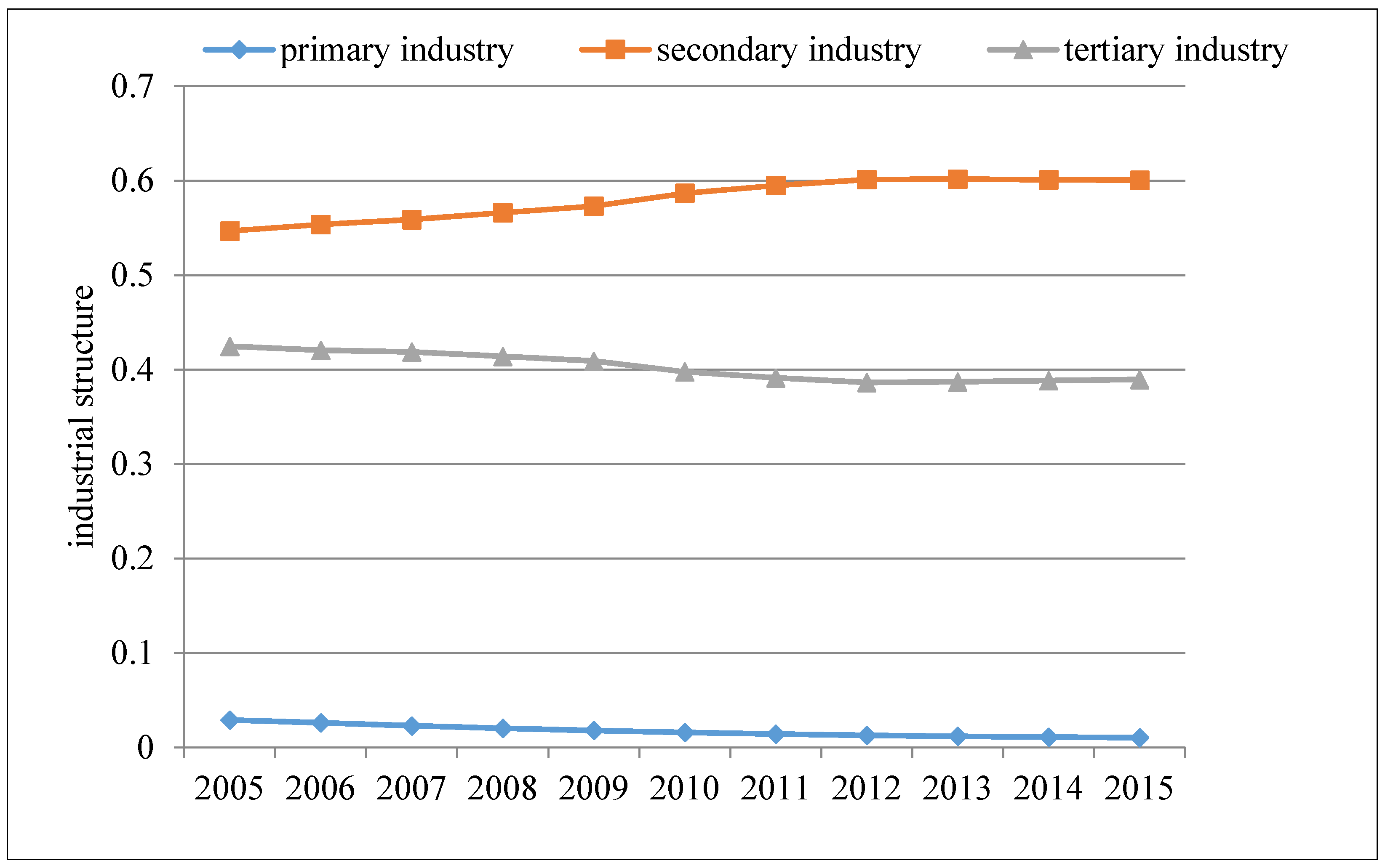
• The industrial structure effect was the main factor driving the decoupling between industrial water utilization and economic growth. The decline in the proportion of primary industry was the main reason for the decline of industrial water utilization. Tianjin’s current industrial structure was “tertiary, secondary, primary”; the proportion of added value from high water-consuming and low-yield primary industries was less than 1.5%. In contrast, the proportion of water utilization was as high as 65%. The proportion of added value from low water-consuming and high-yield tertiary industries was low. As such, there remains significant water-saving potential by optimizing the industrial structure and increasing the representation of the tertiary industry.
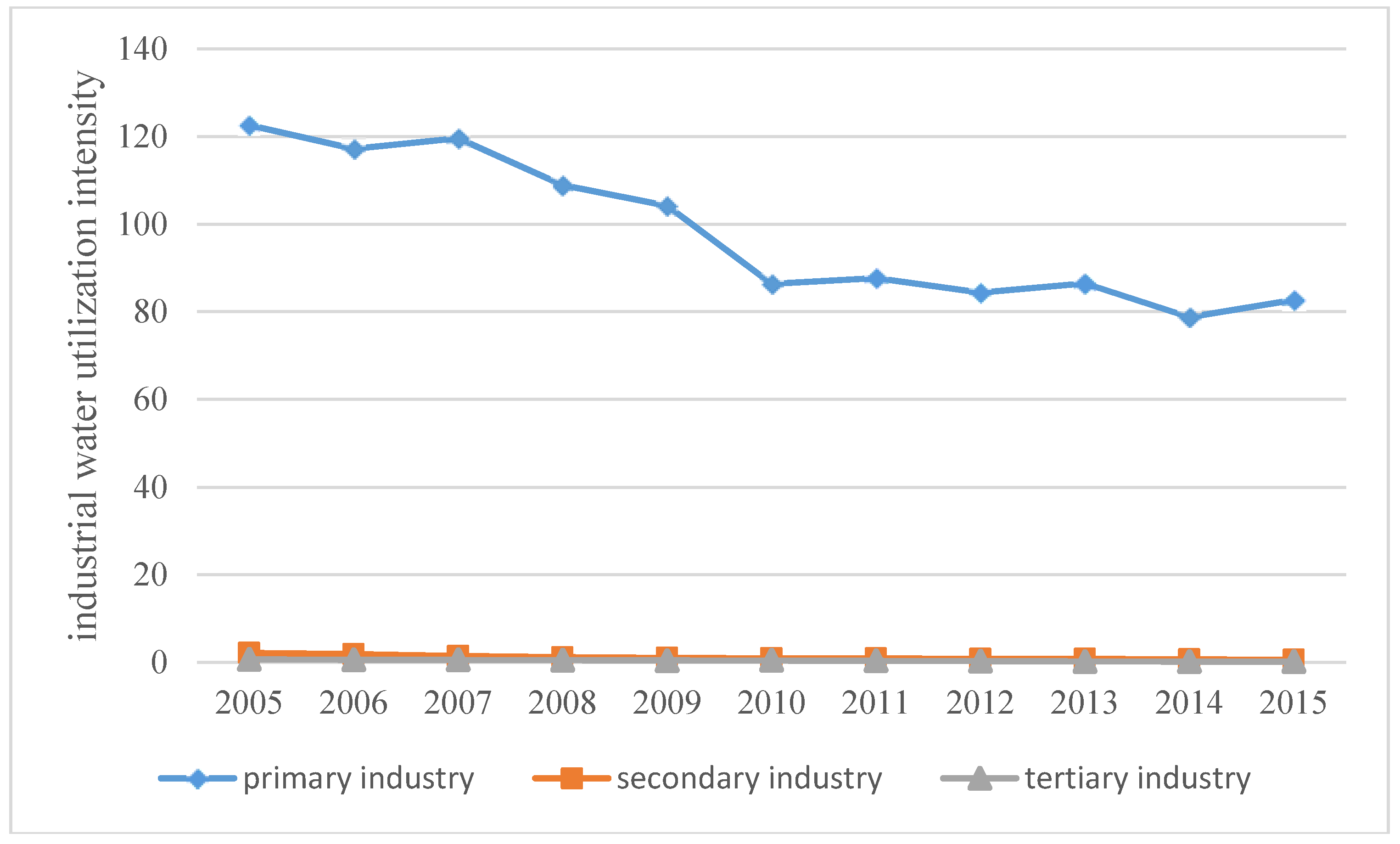
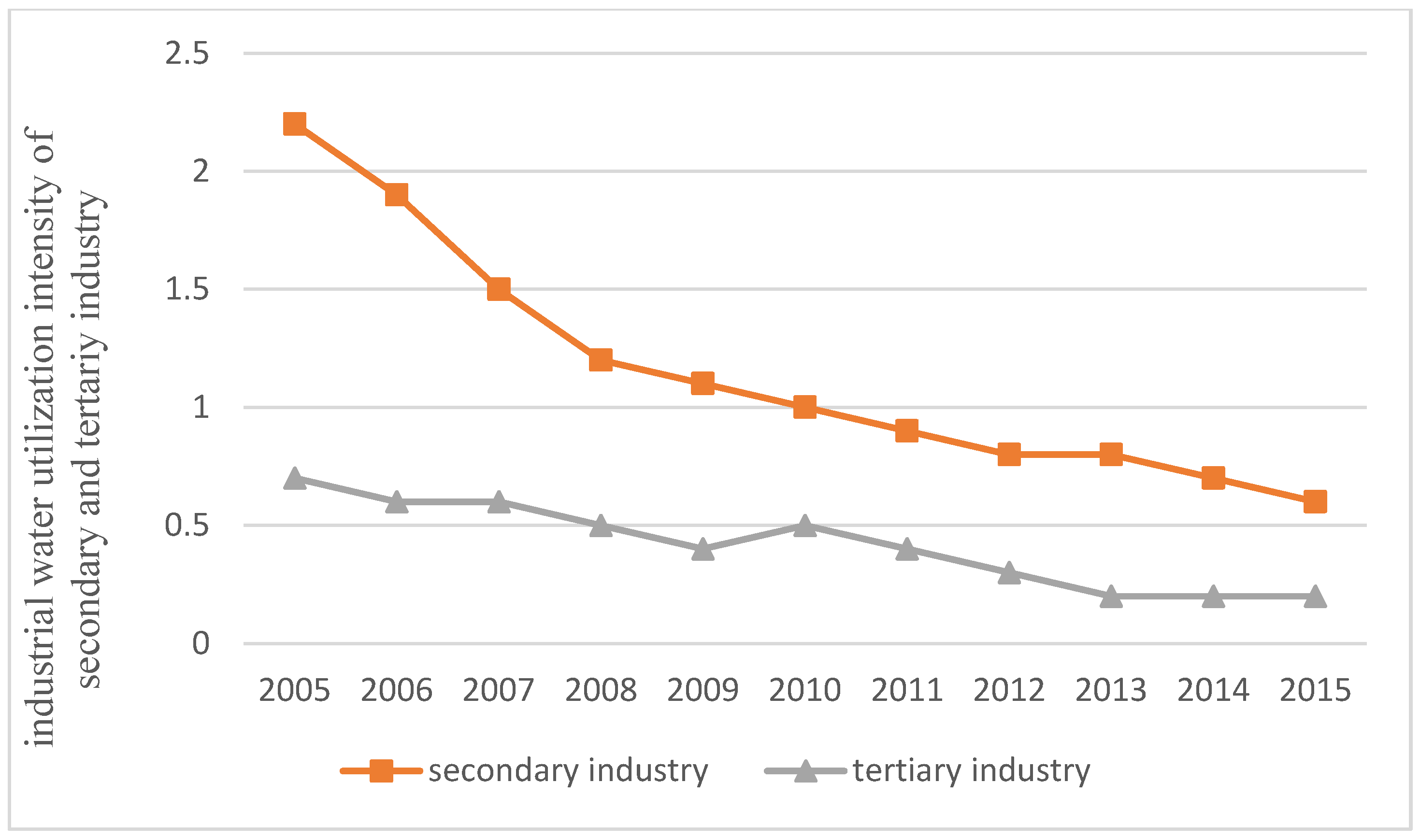
• The industrial water intensity effect steadily drove the decoupling of industrial water utilization from economic growth. During the study period, the industrial water utilization intensity of all three major industries decreased. However, the industrial water utilization intensity of primary industry remained high. Emphasizing reductions in the water utilization intensity of primary industry would help reduce the total volume of industrial water consumed.

Based on study results, the following actions are recommended to better achieve the decoupling of the total volume of industrial water utilization and economic growth.

• Strengthen the control of water utilization and improve the water resource utilization rate. It is important to target high water-consuming primary industries to implement water resources management practices that combine total quantity control and quota management. This would actively improve basic water supply facilities, treat wastewater and sewage and recycle reclaimed water using advanced technology and improve the efficiency of water resources utilization.
• Rapidly optimize the industrial structure and optimize water resource allocation. The changes in the industrial structure have a driving effect on economic growth and industrial water utilization decoupling. We recommend promoting industrial development from a low to high level, increasing the proportion of low water-consuming and high added value tertiary industries, such as financial services and foreign trade. We also recommend transforming economic development patterns and maximizing the construction of a water-saving society.
• Apply water-saving technology and reduce the intensity of industrial water utilization. Industrial water utilization intensity is an important factor driving the decoupling of industrial water utilization and economic growth. Decreasing the water utilization intensity means decreasing the water utilization per GDP. We also recommend improving the efficiency of agricultural irrigation, by adopting water-saving irrigation technologies such as sprinkler irrigation, micro irrigation and drip irrigation; developing and popularizing advanced technology of low water utilization and eliminating the capacity that does not meet standards.

References

1. The Organisation for Economic Co-operation and Development (OECD). OECD Environmental Indicators: Development, Measurement and Use; The Organisation for Economic Co-operation and Development: Paris, France, 2003. [Google Scholar]
2. Toma, P.; Massari, S.; Miglietta, P.P. Life cycle approaches to sustainable regional development. In Life Cycle Approaches to Sustainable Regional Development; Massari, S., Sonnemann, G., Balkau, F., Eds.; Routledge, Taylor & Francis Group: New York, NY, USA, 2016; pp. 143–148. [Google Scholar]
3. Vehmas, J.; Luukkanen, J.; Kaivo-Oja, J. Linking analyses and environmental Kuznets curves for aggregated material flows in the EU. J. Clean. Prod. 2007, 15, 1662–1673. [Google Scholar] [CrossRef]
4. Tapio, P. Towards a theory of decoupling: Degrees of decoupling in the EU and the case of road traffic in Finland between 1970 and 2001. Transp. Policy 2005, 12, 137–151. [Google Scholar] [CrossRef]
5. Wang, Q.; Chen, X. Energy policies for managing China’s carbon emission. Renew. Sustain. Energy Rev. 2015, 50, 470–479. [Google Scholar] [CrossRef]
6. Conrad, E.; Cassar, L. Decoupling Economic Growth and Environmental Degradation: Reviewing Progress to Date in the Small Island State of Malta. Sustainability 2014, 6, 6729–6750. [Google Scholar] [CrossRef]
7. Wei, S. Decoupling cultivated land loss by construction occupation from economic growth in Beijing. Habitat Int. 2014, 43, 198–205. [Google Scholar]
8. Taiyang, Z.; XIanjin, H.; Baiyuan, W. Analysis of decoupling relationship between economic growth and construction land expansion. J. Nat. Resour. 2010, 1, 18–31. [Google Scholar]
9. Schandl, H.; Hatfield-Dodds, S.; Wiedmann, T.; Geschke, A.; Cai, Y.; West, J.; Newth, D.; Baynes, T.; Lenzen, M.; Owen, A. Decoupling global environmental pressure and economic growth: Scenarios for energy use, materials use and carbon emissions. J. Clean. Prod. 2016, 132, 45–56. [Google Scholar] [CrossRef]
10. Lamastra, L.; Miglietta, P.P.; Toma, P.; De, L.F.; Massari, S. Virtual water trade of agri-food products: Evidence from italian-chinese relations. Sci. Total Environ. 2017, 599–600, 474–482. [Google Scholar] [CrossRef] [PubMed]
11. Naqvi, A.; Zwickl, K. Fifty shades of green: Revisiting decoupling by economic sectors and air pollutants. Ecol. Econ. 2017, 133, 111–126. [Google Scholar] [CrossRef]
12. Wang, Q.; Li, R. Journey to burning half of global coal: Trajectory and drivers of China’s coal use. Renew. Sustain. Energy Rev. 2016, 58, 341–346. [Google Scholar] [CrossRef]
13. Andreoni, V.; Galmarini, S. Decoupling economic growth from carbon dioxide emissions: A decomposition analysis of Italian energy consumption. Energy 2012, 44, 682–691. [Google Scholar] [CrossRef]
14. Freitas, L.C.D.; Kaneko, S. Decomposing the decoupling of CO2 emissions and economic growth in Brazil. Ecol. Econ. 2011, 70, 1459–1469. [Google Scholar] [CrossRef]
15. Longhofer, W.; Jorgenson, A. Decoupling reconsidered: Does world society integration influence the relationship between the environment and economic development? Soc. Sci. Res. 2017, 65, 17–29. [Google Scholar] [CrossRef] [PubMed]
16. Roinioti, A.; Koroneos, C. The decomposition of CO2 emissions from energy use in Greece before and during the economic crisis and their decoupling from economic growth. Renew. Sustain. Energy Rev. 2017, 76, 448–459. [Google Scholar] [CrossRef]
17. Lee, C.M.; Rosalez, E.R. Economic Growth, Carbon Abatement Technology and Decoupling Strategy—The Case of Taiwan. Aerosol Air Qual. Res. 2017, 17, 1549–1557. [Google Scholar] [CrossRef]
18. Zhang, M.; Wang, W. Decouple indicators on the CO2 emission-economic growth linkage: The Jiangsu Province case. Ecol. Indic. 2013, 32, 239–244. [Google Scholar] [CrossRef]
19. Zhou, X.; Zhang, M.; Zhou, M.; Zhou, M. A comparative study on decoupling relationship and influence factors between China’s regional economic development and industrial energy–related carbon emissions. J. Clean. Prod. 2016, 142, 783–800. [Google Scholar] [CrossRef]
20. Wang, Q.; Chen, X.; Jha, A.N.; Rogers, H. Natural gas from shale formation—The evolution, evidences and challenges of shale gas revolution in United States. Renew. Sustain. Energy Rev. 2014, 30, 1–28. [Google Scholar] [CrossRef]
21. Diakoulaki, D.; Mandaraka, M. Decomposition analysis for assessing the progress in decoupling industrial growth from CO2 emissions in the EU manufacturing sector. Energy Econ. 2007, 29, 636–664. [Google Scholar] [CrossRef]
22. Lu, I.J.; Lin, S.J.; Lewis, C. Decomposition and decoupling effects of carbon dioxide emission from highway transportation in Taiwan, Germany, Japan and South Korea. Energy Policy 2007, 35, 3226–3235. [Google Scholar] [CrossRef]
23. Zi, T.; Jie, S.; Shi, C.B.; Zheng, L.; Bi, K.X. Decoupling indicators of CO2 emissions from the tourism industry in China: 1990–2012. Ecol. Indic. 2014, 46, 390–397. [Google Scholar]
24. Wang, Q.; Jiang, X.-T.; Li, R. Comparative decoupling analysis of energy-related carbon emission from electric output of electricity sector in Shandong Province, China. Energy 2017, 127, 78–88. [Google Scholar] [CrossRef]
25. Zhu, H.L.; Pan, L.J.; Li, W.Y. Decoupling relationship between water use and economic development in yunnan and guizhou provinces during the first ten years of the great western development strategy. South-to-North Water Transf. Water Sci. Technol. 2013, 11, 1–5. [Google Scholar]
26. Urama, K.C.; Bjørnsen, P.K.; Riegels, N.; Vairavamoorthy, K.; Herrick, J.; Kauppi, L.; Mcneely, J.A.; Mcglade, J.; Eboh, E.; Smith, M. UNEP IRP Report—Options for Decoupling Economic Growth from Water Use and Water Pollution—Factsheet; United Nations Environment Programme: Paris, France, 2016. [Google Scholar]
27. Arto, I.; Andreoni, V.; Rueda-Cantuche, J.M. Global use of water resources: A multiregional analysis of water use, water footprint and water trade balance. Water Resour. Econ. 2016, 15, 1–14. [Google Scholar] [CrossRef]
28. Paolo Miglietta, P.; De Leo, F.; Toma, P. Environmental Kuznets curve and the water footprint: An empirical analysis. Water Environ. J. 2017, 31, 20–30. [Google Scholar] [CrossRef]
29. Miglietta, P.P.; Morrone, D.; Leo, F.D. The Water Footprint Assessment of Electricity Production: An Overview of the Economic-Water-Energy Nexus in Italy. Sustainability 2018, 10, 228. [Google Scholar] [CrossRef]
30. Pellicer-Martínez, F.; Martínez-Paz, J.M. The Water Footprint as an indicator of environmental sustainability in water use at the river basin level. Sci. Total Environ. 2016, 571, 561–574. [Google Scholar] [CrossRef] [PubMed]
31. Sallam, O.M. Water footprints as an indicator for the equitable utilization of shared water resources: (Case study: Egypt and Ethiopia shared water resources in Nile Basin). J. Afr. Earth Sci. 2014, 100, 645–655. [Google Scholar] [CrossRef]
32. Achour, H.; Belloumi, M. Decomposing the influencing factors of energy consumption in Tunisian transportation sector using the LMDI method. Transp. Policy 2016, 52, 64–71. [Google Scholar] [CrossRef]
33. Carmona, M.J.C.; Collado, R.R. LMDI decomposition analysis of energy consumption in Andalusia (Spain) during 2003–2012: The energy efficiency policy implications. Energy Effic. 2016, 9, 1–17. [Google Scholar]
34. González, P.F.; Landajo, M.; Presno, M.J. Multilevel LMDI decomposition of changes in aggregate energy consumption. A cross country analysis in the EU-27. Energy Policy 2014, 68, 576–584. [Google Scholar] [CrossRef]
35. Martínez, C.I.P.; Silveira, S. Energy Use in Manufacturing Industries Evidence from Sweden. 2013. Available online: https://link.springer.com/chapter/10.1007/978-3-642-37753-2_39 (accessed on 23 April 2018).
36. Wang, Q.; Li, R. Drivers for energy consumption: A comparative analysis of China and India. Renew. Sustain. Energy Rev. 2016, 62, 954–962. [Google Scholar] [CrossRef]
37. Cansino, J.M.; Sánchez-Braza, A.; Rodríguez-Arévalo, M.L. Driving forces of Spain’s CO2 emissions: A LMDI decomposition approach. Renew. Sustain. Energy Rev. 2015, 48, 749–759. [Google Scholar] [CrossRef]
38. Mahony, T.O. Decomposition of Ireland’s carbon emissions from 1990 to 2010: An extended Kaya identity. Energy Policy 2013, 59, 573–581. [Google Scholar] [CrossRef]
39. Moutinho, V.; Moreira, A.C.; Silva, P.M. The driving forces of change in energy-related CO2 emissions in Eastern, Western, Northern and Southern Europe: The LMDI approach to decomposition analysis. Renew. Sustain. Energy Rev. 2015, 50, 1485–1499. [Google Scholar] [CrossRef]
40. Oh, I.; Wehrmeyer, W.; Mulugetta, Y. Decomposition analysis and mitigation strategies of CO emissions from energy consumption in South Korea. Energy Policy 2010, 38, 364–377. [Google Scholar] [CrossRef]
41. Timilsina, G.R.; Shrestha, A. Factors affecting transport sector CO2 emissions growth in Latin American and Caribbean countries: An LMDI decomposition analysis. Int. J. Energy Res. 2009, 33, 396–414. [Google Scholar] [CrossRef]
42. Wang, Q.; Li, R. Decline in China’s coal consumption: An evidence of peak coal or a temporary blip? Energy Policy 2017, 108, 696–701. [Google Scholar] [CrossRef]
43. Zhao, C.; Chen, B. Driving force analysis of the agricultural water footprint in China based on the LMDI method. Environ. Sci. Technol. 2014, 48, 12723–12731. [Google Scholar] [CrossRef] [PubMed]
44. Zhang, Y.F.; Yang, D.G.; Tang, H.; Liu, Y.X. Analyses of the changing process and influencing factors of water resource utilization in megalopolis of arid area. Water Resour. 2015, 42, 712–720. [Google Scholar] [CrossRef]
45. Hoekstra, R.; van den Bergh, J.C.J.M. Comparing structural decomposition analysis and index. Energy Econ. 2003, 25, 39–64. [Google Scholar] [CrossRef]
46. Ang, B.W. Decomposition analysis for policymaking in energy: Which is the preferred method? Energy Policy 2004, 32, 1131–1139. [Google Scholar] [CrossRef]
47. Sun, J.W. Changes in energy consumption and energy intensity: A complete decomposition model. Energy Econ. 1998, 20, 85–100. [Google Scholar] [CrossRef]
48. Kaya, Y. Impact of Carbon Dioxide Emission Control on GNP Growth: Interpretation of Proposed Scenarios; IPCC Energy and Industry Subgroup, Response strategies Working Group: IPCC: Paris, France, 1990. [Google Scholar]
49. Tianjin Water Authority. Tianjin Water Resources Bulletin; Tianjin Water Auhtority: Tianjin, China, 2005–2015. [Google Scholar]
50. Tianjin Bureau of Statistics. Tianjin Statistical Yearbook 2016; China Statistics Press: Beijing, China, 2016. [Google Scholar]
Figure 1. Changes in industrial structures in Tianjin during 2005–2015.
Sustainability 10 01323 g001
Figure 2. Changes in the water utilization intensity of three industries in Tianjin during 2005–2015.
Sustainability 10 01323 g002
Figure 3. Changes in the water utilization intensity of secondary and tertiary industries in Tianjin during 2005–2015.
Sustainability 10 01323 g003