Article

Simulating Spatial-Temporal Changes of Land-Use Based on Ecological Redline Restrictions and Landscape Driving Factors: A Case Study in Beijing

1
State Key Joint Laboratory of Environmental Simulation and Pollution Control, School of Environment, Beijing Normal University, Beijing 100875, China
2
Chinese Academy for Environmental Planning, Ministry of Environmental Protection, Beijing 100012, China
*
Author to whom correspondence should be addressed.
Sustainability 2018, 10(4), 1299; https://doi.org/10.3390/su10041299
Submission received: 18 March 2018 / Revised: 19 April 2018 / Accepted: 20 April 2018 / Published: 23 April 2018
(This article belongs to the Special Issue Sustainable Land Uses and Rural Governance)

Abstract

:
A change in the usage of land is influenced by a variety of driving factors and policies on spatial constraints. On the basis of considering the conventional natural and socio-economic indicators, the landscape pattern indicators were considered as new driving forces in the conversion of land use and its effects at small regional extent (CLUE-S) model to simulate spatial and temporal changes of land-use in Beijing. Compared with traditional spatial restrictions characterized by small and isolated areas, such as forest parks and natural reserves, the ecological redline areas increase the spatial integrity and connectivity of ecological and environmental functions at a regional scale, which were used to analyze the distribution patterns and behaviors of land use conversion in the CLUE-S model. The observed results indicate that each simulation scenario has a Kappa coefficient of more than 0.76 beyond the threshold value of 0.6 and represents high agreements between the actual and simulated land use maps. The simulation scenarios including landscape pattern indicators are more accurate than those without consideration of these new driving forces. The simulation results from using ecological redline areas as space constraints have the highest precision compared with the unrestricted and traditionally restricted scenarios. Therefore, the CLUE-S model based on the restriction of ecological redline and the consideration of landscape pattern factors has shown better effectiveness in simulating the future land use change. The conversion of land use types mainly occurred between construction land and cropland during the period from 2010 to 2020. Meanwhile, a large number of grasslands are being changed to construction lands in the mountain towns of northwest Beijing and large quantities of water bodies have disappeared and been replaced by construction lands due to rapid urbanization in the eastern and southern plains. To improve the sustainable use of land resources, it is necessary to adopt the construction and development mode of satellite towns rather than encouraging a disorderly expansion of downtown areas.

1. Introduction

Land-use and land-cover change (LUCC) is considered one of the most profound terrestrial surface changes induced by human activities [1,2]. LUCC emerges from the dynamic interactions between natural and socioeconomic systems, which is identified as a core research field of the studies related to global environmental change [3,4]. Land-use activities caused by needs of development and construction are changing the function and structure of land systems [5]. In urban areas, the conversions from non-construction lands to construction lands represent the most major process and critical form of LUCC [6,7,8,9], which has inevitably brought about negative effects on the landscape pattern and ecological system and put enormous pressure on natural resources and biodiversity [10,11].
With the acceleration of urbanization in China, the acquisition of construction lands for immediate development needs is generally achieved at the expense of degradation of ecological conditions. Frequent and intensive land-use activities have far-reaching consequences for local ecosystems. Reconciling conflicts between ecological conservation and urban development are one of the most formidable challenges encountered in the rapidly developing megacities such as Beijing [12,13,14]. Following this, the concept of ecological redline was first put forward in China during 2011 and was written into Chinese environment protection law in 2014. The implementation of ecological redline policy has been raised to the national strategic level. Ecological redline, recognized as the baseline area of eco-environment system, can provide essential services for the guarantee and maintenance of eco-security and living environment safety [15]. This policy sets rigorous targets for LUCC, which includes that the area cannot be decreased, function cannot be reduced and nature cannot be changed in ecological redline areas. It helps decision-makers to further fill the knowledge gap of “where there can be an orderly development and where there must be strict protection.”
Currently, local and international researchers have carried out related research studies to analyze driving forces and the underlying mechanisms of LUCC [16,17]. Different qualitative and quantitative methods were used to detect the drivers of LUCC [18]. The driving forces of LUCC could be summarized into geographical and socio-economic factors. The former often refers to altitude, slope, aspect and distance to settlements, roads, rails, rivers and green lands; the latter mainly comprises of a city’s GDP, population growth and density. These factors affect land use changes directly or indirectly with high confidence levels [19,20,21,22,23]. Most of existing studies have focused on the response of LUCC to geographical, social and economic drivers, which can provide a reliable reference for simulation of LUCC. Changes in landscape patterns resulting from the usage of land for diverse activities could be a potential reason for non-constructive land fragmentation [24]. The abundance and variety of patch types are the greatest threats to the integrity of lands with ecological functions as well as to the creation of potential conditions for the conversion from non-constructive lands to constructive lands [25,26]. Therefore, ignoring the impacts of landscape pattern dynamics arguably conceals several inherent characteristics of LUCC in spatial distributions. Ecological redline aims to protect the important eco-fragile hotspots and eco-functional areas. It attempts to select the ecosystem services as a way to restrict unreasonable land-use activities compared to the existing restricted areas such as nature reserves, scenic resorts and wetlands. Few studies have been found in the literature that take into account the ecological redline as spatial restriction due to the novelty of the proposed policy. Therefore, it is well worth simulating the land-use changes restricted through ecological redline, which is expected to provide a comprehensive understanding of LUCC.
A variety of models have been widely introduced and exploited to simulate land use changes, such as cellular automata (CA) [27,28], agent-based modeling (ABM) [11] and conversion of land use and its effects modelling (CLUE) [29]. As a tool to simulate the spatio-temporal dynamics of complex systems, the CA model has been extensively used in the study of land use change and urban growth [30]. CA models are not determined by strictly-defined physical and mathematical equations or functions and thus they are simpler and more flexible in their simulation of LUCC. Given the spatial and temporal complexities of LUCC, it is not enough to simulate changes of land use by properly defining conversion rules in CA models. More and more researchers focus on introducing constraints and building models, for example the SLEUTH model developed based on the CA model, to simulate land use changes more realistically [31,32]. However, the CA model has worse performance in simulating multiple land use changes. When different land uses are presented, the simulation involves more spatial variables and parameters and makes conversion rules and model structures more complicated [33]. The process of LUCC is not only associated with natural constraints but also related to human drivers. In the context of ABM, diverse actions and decisions of human are incorporated into modeling of LUCC. The model provides a further understanding of the relationship between human drivers and causal mechanisms of LUCC. However, the main challenge of ABM is to clarify specific interactions between human actors and land systems, especially different response mechanisms and decision-making processes at various organizational levels. In the coupled human-environmental systems, the intrinsic complexity of interactions is so multifaceted that researchers have been exploring an effective approach to explicitly capture human behavior on LUCC [11,34]. The CLUE model was developed to simulate and predict the spatial changes in land-use pattern [29,35]. The CLUE-S version has been mainly used at smaller regional scale instead of larger national extent. It can quantitatively analyze spatial-temporal dynamics of multi-type land-use, particularly simulating possible land changes under a set of specified scenarios and considering driving forces, neighborhood elements and land suitability related to the designed scenarios. Because of its ease of implementation and its ability to simulate multiple land use changes combined with dynamic modelling of competition between different land types, the CLUE-S model has been widely applied in local and regional case studies with the spatial resolution varying from 20 to 1000 m [36,37,38].
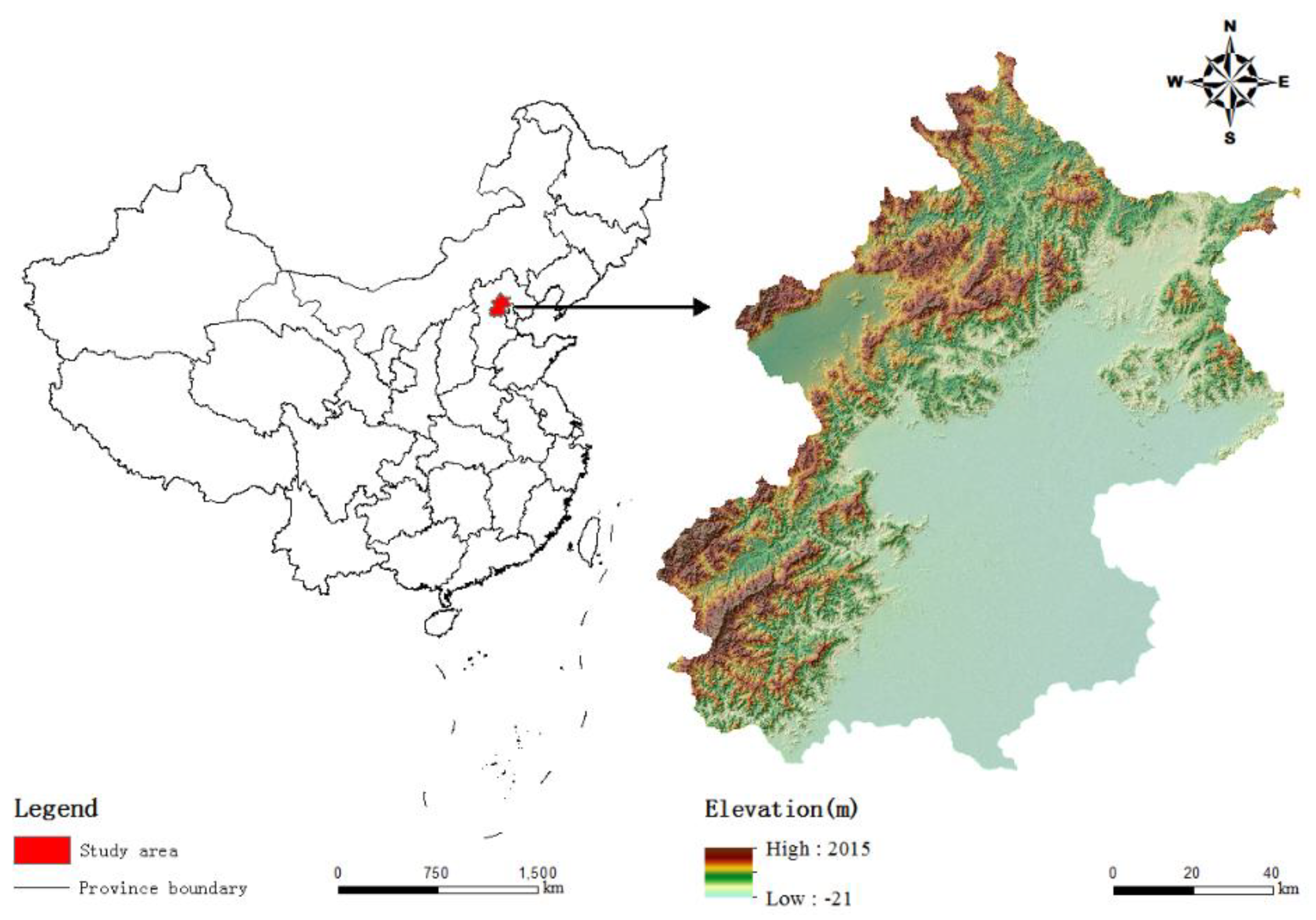
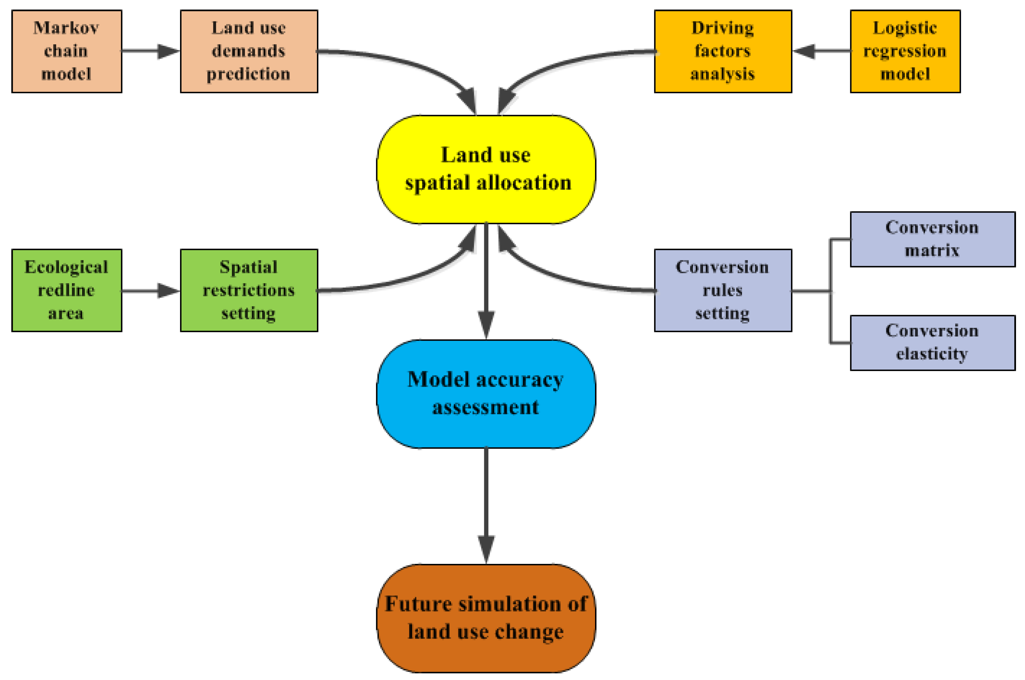
In this study, a CLUE-S model restricted by ecological redline is developed, which also takes into account the landscape metrics based on previous driving forces. The Kappa coefficient is introduced to evaluate the quality and to confirm the validation of the selected model as compared with the models with no restriction areas and traditional restriction areas such as nature reserves. We also apply the model to simulate spatio-temporal changes of land use in Beijing. The result can provide a scientific reference and strategic decision for promoting sustainable urban development.

2. Materials and Methods

2.1. Study Area

Beijing is located at longitude 115.7°–117.4° east and latitude 39.4°–41.6° north (Figure 1). It covers an area of 16,411 km2 with the gradual declination of altitude from northwest to southeast. The permanent population of Beijing increased from 15.4 to 21.7 million between 2005 and 2015, of which approximately 86.5% was urban. The GDP increased from 696.9 to 2301.5 billion RMB over the same period (Beijing Statistical Yearbook, 2016). These changes are related to the rapid urbanization process and corresponding expansion of construction land. Construction land accounted for 21.5% of the total area in 2015. During the same period, Beijing experienced severe degradation of ecosystems. For instance, the wetland area reduced from 4.07% to 1.86% between 1978 and 2005 [39]. There exists an intense conflict between urban development and ecological protection. Scientific land-use planning is urgently carried out to minimize negative ecological impacts during the process of urban expansion.

2.2. Data Sources

Landsat Thematic Mapper (TM) and Enhanced Thematic Mapper Plus (ETM+) images of 2010 and 2015 with a resolution of 30 m were interpreted by researchers to retrieve the types of land-cover. The main steps of data preprocessing included radiation calibration, geometric correction and image mosaic. Land-use types were categorized into 5 classes: croplands, forestlands, grasslands, water bodies and construction lands [40]. The data of terrain and elevation were derived from Shuttle Radar Topography Mission Digital Elevation Model (SRTM DEM) data through the Geospatial Data Cloud Platform (http://www.gscloud.cn/) for slope and aspect extraction, which had a spatial resolution of 90 m. Vegetation index data were also obtained from the Geospatial Data Cloud Platform. Socio-economic data were available from the Beijing Statistical Yearbook.

2.3. CLUE-S Model

The CLUE-S model was used in this study to simulate dynamics of land cover types. It was developed by Wageningen University to simulate explicitly the spatial-temporal land use changes that were specified in certain scenarios. The simulation is based upon the competition of different types of land resources and the location suitability combined with empirical analysis. CLUE-S is divided into the spatial module and non-spatial module. The spatial allocation part includes land use patterns, driving factors, conversion matrix, conversion elasticity and spatial restrictions. The spatial module decides land use changes in different grid cells and needs to be consistent with demands for all types of land resources calculated in the module of non-spatial analysis. The proposed CLUE-S model is often validated by comparing the simulation results with the actual changes of land use. Then, the model can be used to simulate future land use change. An overview of the CLUE-S model is shown in Figure 2.

2.3.1. The Prediction on Land-Use Demands

Land use requirements refer to area changes of all kinds of land-cover types at an aggregate level in the study region. The Markov Chain model describes a dynamic process in which various lands can be converted into each other and transition rates are comparatively stable during certain periods. The probability distribution of land-use in the next status in the model is determined by the current state instead of previous ones [41]. The Markov Chain has been adopted widely to predict temporal changes of land use in a large number of studies [42,43,44]. The matrix of land-use transition probability is first required to be calculated by expressions and requirements as follows:
p = ( p i j ) = [ p 11 p 12 p 1 n p 21 p 22 p 2 n p n 1 p n 2 p n n ]
0 p i j 1 ( i , j = 1 , 2 , , n )
i = 1 n p i j = 1 ( i , j = 1 , 2 , , n )
where p i j is transition probability of the ith type of land into the jth type of land from the current state to next state; n is the total amount of types of land resources; the sum of transition probability is 1.
According to the transition probability matrix and non-after effect of process, the expression of Markov Chain is written as follows [41,44]:
p m = p m 1 p i j
where p m is the probability of state at any moment; p m 1 is the probability of the previous state. The transition rates and dynamic processes of all land types were operated by spatial analysis module in ArcGIS 10.1. The prediction of land-use demands spans 10 years in which two years nodes of 2010 and 2015 were employed to calculate a matrix of transition probability. Successively, land-use requirements in each period were obtained based on the Markov Chain model (Table 1).

2.3.2. Driving Factors Analysis

Land use conversions tend to take place for specific land-use types with the highest “preferences”. The preference reveals the spatial differences of land configuration resulting from interactions of different decision-making processes. The preference is analyzed and estimated by a set of driving factors derived from understandings of land-use change determinants. In the simulation process, logistic regression is an important step aiming to examine relationships between driving forces and the spatial distribution of categories of land use. Variables that make an insignificant contribution to the interpretation of land spatial allocation will be removed from the equation of logistic regression [45]. Once the occurrence probabilities have been calculated, significant driving factors will be retained and insignificant ones will be eliminated [35]. The logistic regression equation was applied in the study to estimate contributions of a wide range of driving factors and further determine the location suitability of a specific type of land resource in a certain grid cell. The logistic regression equation is expressed as follows [29]:
log ( P i 1 P i ) = β 0 + β 1 X 1 + β 2 X 2 + + β n X n
where P i is the occurrence probability of a specific type of land resource in a certain grid cell; X n is the nth driving factor; β 0 is the constant; β n is the coefficient of the nth driving factor.
Driving factors can be generally divided into natural and socio-economic components, which exert a direct or indirect influence on land use conversions. Grid cells can represent natural differences, whereas the administrative units represent the socio-economic differences. The variables are introduced to assess the suitability of a certain location devoted to a specific type of land resource. The natural driving factors obtained include DEM, slope, aspect, vegetation index and distances data to administrative centers, main roads, metro lines, rivers and green land. Distances data were obtained using the tool of “Euclidean Distance” in ArcGIS 10.1. Socio-economic driving factors include GDP, population density and permanent migrant population.
With an increase in the activity of human beings, the frequent and dramatic changes of land use have caused enormous pressures on the integrity of landscape. Landscape fragmentation, in turn, emerges as an important stimulus due to which the geographical and functional relationships of the specified land type are ruptured. The abundance and variety of patch types create potential conditions for land use conversions. Therefore, ignoring the impacts of landscape pattern dynamics possibly conceals several inherent characteristics of LUCC in spatial distributions. Evaluation of the impacts of landscape fragmentation degree on land use changes is essential for urban planning and the management of land resources. Landscape fragmentation describes the land-use spatial structure and provides information about land-use categories in the given region. In this context, landscape fragmentation indicators can be used as valuable variables to quantify the occurrence probability and contribute to improving and enhancing the knowledge of land-use changes [24,25]. In the study, the driving factors of landscape fragmentation include patch densities (PD) of croplands, forestlands, grasslands, water bodies, construction lands and Shannon’s diversity index (SHDI). Landscape fragmentation indicators were calculated by using the software FragStats4.2.
5000 random points within the scope of Beijing were created applying the tool of “Create Random Points” in ArcGIS 10.1. Then values of driving factors were obtained adopting the tool of “Extract Values to Points.” Values of coefficients ( β n ) and constants ( β 0 ) were confirmed by the SPSS20.0. The obtained results have been shown in Table 2.

2.3.3. Settings in the Spatial Restrictions

Spatial restrictions mostly refer to certain areas where changes in land use are restricted based on spatial policies. They can influence spatio-temporal distribution patterns and behaviors of land use conversion. In the CLUE-S, spatial restrictions refer to traditional spatial limitation areas. In general, spatial restrictions play important roles in protecting the designated targets such as natural reserves, scenic spots, historical relics and potable water sources. Large numbers of these areas are small and isolated. Moreover, boundaries of areas are adjusted frequently to satisfy the demands of development and construction [15]. Ecological redline is defined as an insurmountable baseline area, which aims at protecting and maintaining the integrity of important systems to meet different ecological and environmental needs. The ecological redline policy consists of following main objectives. Firstly, protecting the important function areas that can provide services including ecological safety, water storage and clean drinking water to support social and economic developments. Secondly, protecting eco-fragile areas such as regions characterized by soil erosion and land desertification in order to maintain the safety of the human living environment. Thirdly, protecting habitats for important species and maintaining biodiversity. The policy of ecological redline is beneficial for solving spatial mismatches and isolations caused by traditional spatial restrictions and the spatial connectivity will be increased at a regional and national scale. Ecological redline is considered as a mandatory policy and a strict measure for the protection of eco-environment system. Any activity of construction and development will be prohibited within ecological redline areas. Focusing on the large territories covered by the ecological redline policy, rather than the protection of hotspots, will help the city planners and managers in knowing the spatially explicit boundaries of where there can be an orderly development and where there must be strict protection [13,46].

2.3.4. Conversion Rules

In the CLUE-S model, conversion rules include the conversion matrix and conversion elasticity. The conversions that could occur possibly and impossibly are defined in a matrix of land use conversion. The conversion matrix indicates any type of land can be transformed into other types of land. If the value in the conversion matrix is “1”, it means the conversion occurs. However, a value of “0” indicates that land use transition is not possible. In this study, all conversions of land-use types are possible and rows and columns of the conversion matrix are 1. The elasticity of conversion is associated with the reversibility of land use conversions. A certain type of land with irreversible environmental impacts or high capital investment can be difficultly transformed into other types. Therefore, this category is more stable and static than other ones. The conversion elasticity varies from 0 to 1. The higher the conversion elasticity, the more difficult it is for this land type to be changed. The conversion elasticity of each land use type is shown in Table 3.

2.3.5. Land Spatial Allocation

The allocation of land demands to every grid cell continues until allocated goals have been achieved by comparing acquired areas of the specified type of land with required areas iteratively. The competitive advantage for each kind of land type is determined in the iterative process. Values will be increased when the acquired area is not enough for the required area, whereas values will be decreased when the acquired area is larger than the required area in the process of the iteration. Higher values will be obtained with the increase of demand for the specified land type. For a specified land type, total probability in each cell can be calculated by the expression as follows [29]:
T P R O R i , n = P i , n + E L A C n + I T E R n
where T P R O R i , n is the total probability of ith unit for nth land; P i , n is the occurrence probability of nth land for ith unit; E L A C n is the conversion elasticity of nth land; I T E R n is the iteration variable of nth land.

2.3.6. Assessment on the Model Accuracy

The accuracy of CLUE-S is commonly validated through the comparison of simulated results with the actual results of land-use changes over a certain historic period [47]. In this study, the Kappa coefficient was introduced to assess the accuracy and effectiveness of the simulation results. The land-use simulation result in 2015 was obtained based upon the actual map of land-use in 2010 and a comparison was carried out with the actual land use in 2015. The expression of the Kappa coefficient is generally shown as follows [48]:
K a p p a = P o P c P p P c
where P o is the observed correct proportion; P c is the expected correct proportion; P p is the absolute correct proportion. The Kappa coefficient ranges from 0 to 1. The value closer to 1 represents a higher similarity or stronger agreement between the simulation result and the actual map. A Kappa coefficient beyond 0.8 suggests a strong agreement; the value ranging from 0.6 to 0.8 reveals a high agreement; the value between 0.4 and 0.6 shows a moderate agreement; and when the value is below 0.4, the agreement is poor [44].

3. Results

3.1. Spatial Changes of Land-Use Pattern

There has been substantial shrinkage of the croplands and a remarkable expansion of construction lands from 2010 to 2015 (Figure 3 and Table 4). The total area of construction land increased significantly from 275,457.00 ha in 2010 to 346,971.75 ha in 2015, with an average annual increase of 11,919.12 ha. Due to the rapid process of urbanization, other land-use types were occupied to varying degrees. Each type of non-construction land was encroached between 2010 and 2015. The croplands suffered the most decreased area that reached 37,262.50 ha, accounting for 52.10% of the total decreased area of non-construction lands. This was followed by grassland and water body, which respectively accounted for 21.44% and 16.22%. Most of the land-use conversions occurred between construction land and cropland. In terms of the intensity of land change, the total area of water body declined to 33,284.50 ha in 2015, went down by 25.84% with a loss of 11,596.50 ha during 2010–2015, followed by grassland with 13.10%. Conversion from urban non-construction lands to construction lands was the main process and an important form of LUCC. Frequent and intensive human activities had a negative effect on changes of the structure, pattern and function of the land types.

3.2. Ecological Redline Analysis

Based on the data delimited and provided by the Chinese Academy for Environmental Planning and the Beijing Municipal Research Institute of Environmental Protection, traditional spatial restrictions include forest parks, natural reserves, drinking water source areas, historical and cultural relics and famous landscapes and sceneries (Figure 4). They are mainly situated at the northern and western hills and mountains of Beijing, which aim to protect the specified objectives such as forests, scenic spots, historical relics and potable water sources and so forth. Large numbers of these areas are small and isolated and cannot describe the integrity and connectivity of ecological and environmental functions. Moreover, the results ignore some of the functional areas in the southern and eastern plains, which act as positive feedback to local ecological and environmental systems. Ecological redline areas are categorized into 7 classes: headwater conservation, biodiversity maintaining, vital ecological function, soil and water conservation, drinking water source protection, wind prevention and sand fixation and important natural and artificial landscapes (Figure 4). Headwater conservation areas located in the mountains of north Beijing has the largest area of 212,625.86 ha, accounting for 24.73% of the total ecological redline area, followed by important natural and artificial landscapes with an area of 178,075.14 ha, which is 20.71% (Table 5). In contrast, wind prevention and sand fixation areas are the smallest redline regions, only accounting for 1.32% of the total ecological redline area. These redline areas contain traditionally restricted regions and help resolve the spatial isolations of the common spatial restrictions. Ecological redline areas are more connected geographically and are more consistent functionally than the traditionally restricted regions. The ecological redline areas reveal key ecological functional areas in the southern and eastern plains as compared to the traditionally restricted areas, which increase the spatial integrity and connectivity of ecological and environmental functions at a regional scale.

3.3. Accuracy Assessment of Land Use Simulation

The result for the land use pattern in 2015 was simulated depending on the actual map of land-use in 2010. Six scenarios were established and contrasted, applying the model of CLUE-S from the perspectives of the driving factors of landscape pattern and spatial restrictions (Figure 5), including no spatial restrictions but excluding landscape pattern indicators, traditional spatial restrictions excluding landscape pattern indicators, ecological redline restrictions excluding landscape pattern indicators, no spatial restrictions including landscape pattern indicators, traditional spatial restrictions including landscape pattern indicators and ecological redline restrictions including landscape pattern indicators. The Kappa coefficient was adopted to evaluate the accuracy of simulation results and validate the CLUE-S models.
The overall accuracy of each simulated scenario is above 0.76, ranging from 0.6 to 0.8 (Table 6), which represents a good agreement between the actual map and the simulated result in 2015. The results suggest a high percentage of correctly simulated pixels. Scenarios including landscape pattern indicators show a higher accuracy of the simulation than ones excluding landscape pattern indicators. The abundance and variety of land parcels reveal land-use spatial structure and create potential conditions for inter-transitions of different land-use types. Therefore, landscape pattern indicators have effects on land use changes. In the six scenarios, simulated results based on ecological redline restrictions show the highest accuracy as compared to no spatial restrictions and traditional spatial restrictions. Table 7 shows that every type of land has a Kappa coefficient above 0.6 except for water body, which is approximately 0.6. For each type of land-use, simulated results with ecological redline constraints indicate the highest agreements between actual maps and simulated results in three scenarios specified by different spatial restrictions. Ecological redline policy, as a mandatory and the strictest protection policy, focuses on the large numbers of functional areas with the strongest integrity and connectivity in space instead of protecting some of the hotspots at a regional scale. Ecological redline can describe spatially explicit boundaries where there can be an orderly development and where there must be a strict protection. Therefore, the simulated results based on the ecological redline restrictions, with the consideration of landscape pattern indicators, indicate that the model with these settings can effectively simulate LUCC in the future.

4. Discussion

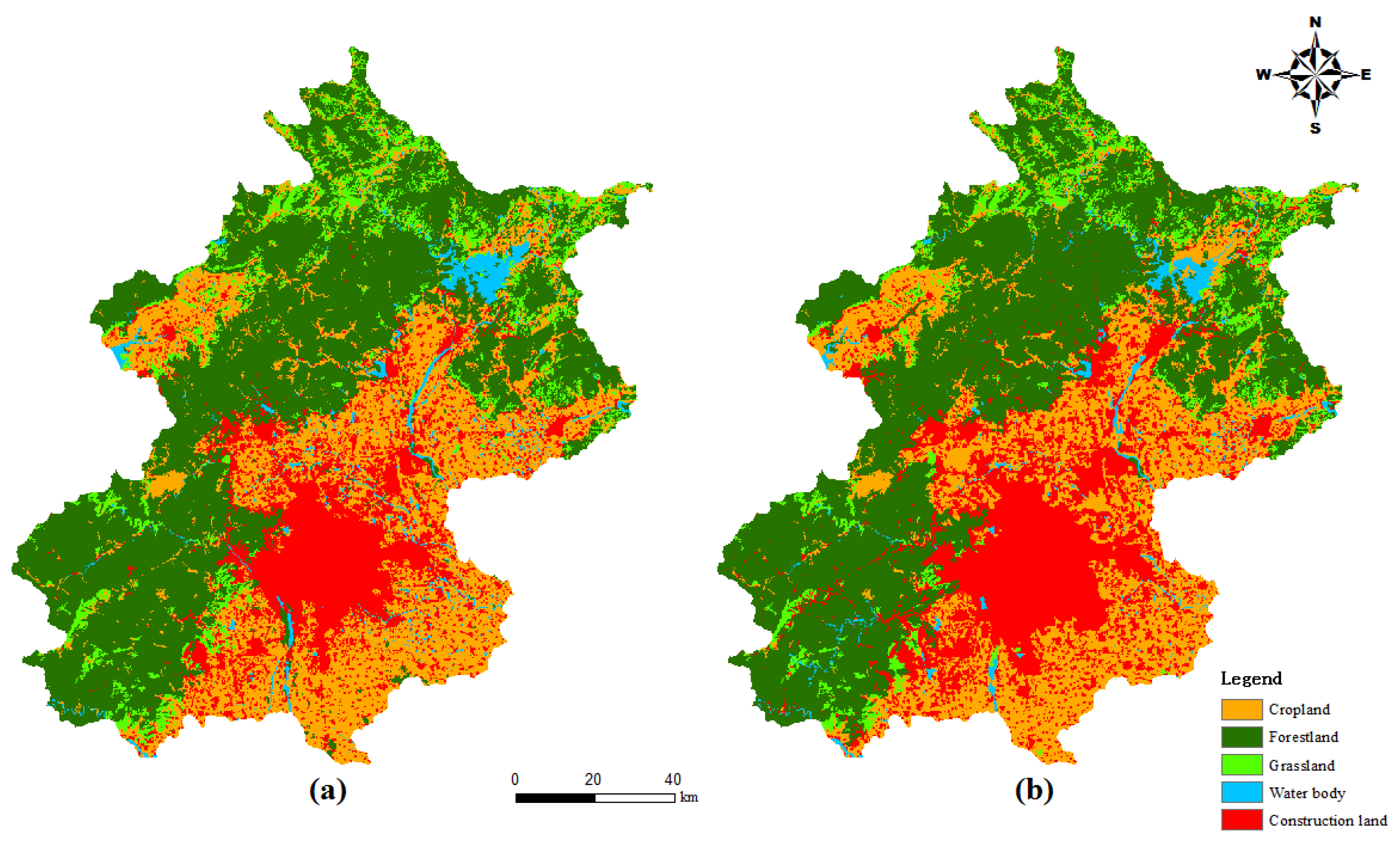
Simulation results confirm a trend that the overall change of land-use in Beijing over the period from 2010 to 2020 focuses on outward expansion around central urban areas, accompanied by the exurban sprawl distributed across multiple counties (Figure 6). This dynamic reflects a spread of human settlements around the central city to the surrounding plains, while the diffusion in mountainous areas is relatively slower and to a much lesser extent. The process of this land-use conversion has been mainly achieved by encroaching on the croplands continuously. There has been a significant encroachment on the croplands and an obvious expansion of construction lands from 2010 to 2020 in the eastern and southern plain of Beijing. In 2010, people’s urban activities and behaviors were mainly concentrated in the central urban areas. In other districts and counties, there was a scattered distribution pattern that did not develop into a larger scale. By 2020, due to the never-ending expansion of the central urban area, the built-up area of the surrounding districts and counties will be expanding, which presents a tendency to gradually connect with the central area and become a spatial agglomeration entity of urban activities at a regional scale. In addition to the large encroachment of croplands, large quantities of grasslands have disappeared and been replaced by construction lands in the mountain towns of northwest Beijing and a significant shrinkage on water bodies occurs due to the rapid urbanization in the eastern and southern plain.
Disorderly spreading of urban space has not only destroyed abundant land resources but also easily triggered a series of problems such as traffic congestion, environmental pollution and population overcrowding. It does not keep in accordance with the goal of sustainable development. Conversely, the development mode of “satellite town” could effectively restrain the undesirable demands of urban sprawl. It depends on the prior urban development of downtown areas and still remains to be independent in order to alleviate the pressures on the population, transportation and industrial development in the central urban areas. According to the result of land use change in Beijing in 2020 simulated by CLUE-S, the decision-makers could take the following measures at the macro level: (1) Implementing stricter ecological redline policy to demarcate spatially explicit boundaries where there can be an orderly development and where there must be a strict protection (2) Encouraging the development and construction of satellite towns in case of overexpansion of downtown areas to ease the high pressures produced by urban sprawl (3) Implementing scientific spatial layout and rational planning of satellite towns to effectively prevent an excessive deterioration and fragmentation of natural landscapes and to restrain the transformation from basic farmlands into construction lands.
With the implementation of Beijing Urban Master Plan (2016–2035) approved by the State Council, Beijing will change the existing urban spatial structure characterized by the single center and focus on the space pattern of multi-center development. In addition, the new planning puts forward definite demands for setting and holding firm to ecological redline and forming a harmonious spatial pattern integrated with mountains, waters, forests, farmlands, lakes and the city in the overall layout. The simulation result, restricted by ecological redline, is most consistent with the actual change of land use from 2010 to 2015, which shows that ecological redline, defined as mandatory space constraint, has been considered in the actual activities of urban planning and management. The CLUE-S model based on ecological redline can simulate future land use changes in a more realistic situation and meet the requirements of the new Beijing Urban Master Plan. According to the simulation result, the obvious expansion trend of the construction land in Beijing’s suburban counties is influenced by the government’s policy of developing new towns, especially in the areas rarely restricted by ecological redline, such as Changping, Shunyi and Miyun. The function of the central urban area is gradually transferred to the suburban counties, which facilitates the formation of a polycentric development pattern. The construction of new towns is an important strategy to attract the population to concentrate in suburban counties and achieve the goal of the balance of population distributing required by Beijing Urban Master Plan.
The model developed in this study considers a comparatively comprehensive driving forces of land-use allocation, which include natural, locational, social, economic and landscape pattern attributes. Landscape pattern factors rarely expressed and described in previous models are considered and simulated in this model. The ecological redline, implemented as the strictest protection policy, sets rigorous requirements for land-use allocation and will play an increasingly important role in future land use changes. Ecological redline areas were restricted as areas with stable functions of land-cover in the simulation, which means that these specific lands in the particular regions were prohibited from all kinds of development and construction activities. The conceptual framework of the CLUE-S model, based on ecological redline restrictions and landscape driving factors, is capable of highlighting the space constraints with spatial integrity and connectivity and potential socio-ecological impacts of urban growth and encroachment on other types of land at the regional scale.
The proposed model can provide a tool for exploring the possible effects related to ecological redline policy and specific landscape pattern factors, which can be used to support further sustainable planning interventions. We believe that the proposed model should be systematically included in practices of spatial planning so as to foster sustainable development at the regional scale. Due to rapid economic growth and urban expansion, conflicts over land resources between humans and nature are continuously increasing [49]. The disordered spatial development and irrational processes in urbanization destroy the essential land systems thereby affecting the local people at this stage and potentially might affect the next generation, which further brings a huge threat to the sustainable development of these regions. Therefore, correct and properly calibrated spatial planning is more necessary than ever; it is precisely through the reduction of soil loss, the protection of drinking water sources and other valuable ecosystems and the preservation of high quality areas for biodiversity and important natural landscapes, that the sustainable abilities can be increased and sustainability targets can be achieved [31]. Additionally, this model also has the merit of having simulated spatially explicit distributions of multiple land use changes, which will be of value in future planning aimed at reducing the loss of non-construction lands for sustainable development in Beijing.
However, a major limitation of this model is the representation of causal mechanisms between driving factors and land-use and land-cover changes. In practice, due to the complexity of land use systems and the diversity of economically, socially and environmentally influencing factors, it is seemingly impossible to assess and analyze all the activities that determine LUCC. The limitation for availability of detailed data results in the lack of elaborate parameterization. In addition, the randomness and uncertainty generated by the limitation increase difficulties of excellent performance and credibility of the model. Therefore, there are several points that can be improved further. Firstly, it is necessary to further explore interactions of land use changes and landscape pattern changes in the model to further find out new driving factors. Secondly, more alternative scenarios should be taken into account, such as scenarios paying attention to economic development and scenario giving priority to environmental protection. Thirdly, the CLUE-S model should be coupled with other methods or models, such as the multi-agent system model, to further improve the accuracy and effectiveness of simulation and prediction.

5. Conclusions

This research featured an application of the CLUE-S model to simulate and analyze past and future land use changes in Beijing, China. We focused on the differences resulting from the application of contrasting scenarios based on spatial restrictions and driving factors. In this paper, on the basis of considering conventional natural and socio-economic indicators, the landscape pattern indicators were considered as new driving forces in the CLUE-S model to simulate spatial and temporal changes of land-use in Beijing. Compared with traditional spatial restrictions characterized by small and isolated areas, such as forest parks and natural reserves, the ecological redline areas increase the spatial integrity and connectivity of ecological and environmental functions at a regional scale, which were used to analyze distribution patterns and behaviors of land use conversion in the CLUE-S model. The validation results show that each simulation scenario has a precision of more than 0.76 and represents a high agreement between the actual map and the simulated result. The simulation scenario based on ecological redline restrictions and landscape driving factors has the highest Kappa coefficient with the value of about 0.7717. The simulation scenarios, including landscape pattern indicators, are more accurate than those without consideration of these new driving forces. The simulation results that use ecological redline areas as space constraints have the highest precision compared with the unrestricted and traditionally restricted scenarios. The CLUE-S model proposed in this paper has shown better effectiveness in simulating future land use change.
In order to simulate a more realistic changes of land use and support the policy decisions of urban development in Beijing, the CLUE-S model based on ecological redline restrictions and landscape driving factors was proposed to forecast and analyze the spatial and temporal dynamics of land at the regional scale. The overall change in Beijing’s land use during the period from 2010 to 2020 concentrates on city-centered outward expansion as well as the exurban sprawl distributed across multiple counties. This change describes an obvious spread of construction lands around the central urban areas to the surrounding plains, while human settlements in the hilly area are expanding at a relatively slower rate and to a much lesser extent. In terms of land-use structure change, land-use conversion mainly occurs between construction land and cropland. A large number of croplands are being converted to construction lands over the period from 2010 to 2020. Moreover, there has been a significant encroachment of grasslands in the mountain towns of northwest Beijing and large quantities of water bodies have disappeared and been replaced by construction lands due to rapid urbanization in the eastern and southern plains. To improve the sustainable use of land resources, it is necessary to adopt the construction and development mode of satellite towns rather than encouraging the disorderly expansion of central urban areas.

Acknowledgments

The authors also would like to acknowledge the contributions of the Beijing Municipal Research Institute of Environmental Protection. The paper was completed with support also from the State Key Joint Laboratory of Environmental Simulation and Pollution Control. The authors thank the anonymous editor for the editing assistance. Lastly, the authors would like to thank the anonymous reviewers for their valuable comments and suggestions on an earlier version of our manuscript.

Author Contributions

Zimu Jia carried out the research and wrote the article as part of a PhD project; Weihua Zeng acted as research co-promoter and contributed to the design of the research proposal and methodology; Bingran Ma and Jing Zhang conducted the data collection and analysis.

Conflicts of Interest

The authors declare no conflict of interest.

Funding

This research was undertaken at the Beijing Normal University, School of Environment and funded by the Innovative Technology Research on Coordinated Development of Regional Economic Construction and Natural Ecological Protection in Multi-type Protected Areas (No. 2017YFC0506403).

References

  1. Turner, B.L.; Lambin, E.F.; Reenberg, A. The emergence of land change science for global environmental change and sustainability. Proc. Natl. Acad. Sci. USA 2007, 104, 20666–20671. [Google Scholar] [CrossRef] [PubMed]
  2. Vitousek, P.M.; Mooney, H.A.; Lubchenco, J.; Melillo, J.M. Human domination of earth’s ecosystems. Science 1997, 277, 494–499. [Google Scholar] [CrossRef]
  3. Aquilué, N.; Cáceres, M.D.; Fortin, M.J.; Fall, A.; Brotons, L. A spatial allocation procedure to model land-use/land-cover changes: Accounting for occurrence and spread processes. Ecol. Model. 2017, 344, 73–86. [Google Scholar] [CrossRef]
  4. Wu, J.G.; Hobbs, R. Key issues and research priorities in landscape ecology: An idiosyncratic synthesis. Landsc. Ecol. 2002, 17, 355–365. [Google Scholar] [CrossRef]
  5. Foley, J.A.; DeFries, R.; Asner, G.P.; Barford, C.; Bonan, G.; Carpenter, S.R.; Chapin, F.S.; Coe, M.T.; Daily, G.C.; Gibbs, H.K. Global consequences of land use. Science 2005, 309, 570–574. [Google Scholar] [CrossRef] [PubMed]
  6. Bürgi, M.; Hersperger, A.M.; Schneeberger, N. Driving forces of landscape change-Current and new directions. Landsc. Ecol. 2004, 19, 857–868. [Google Scholar] [CrossRef]
  7. Luck, M.; Wu, J.G. A gradient analysis of urban landscape pattern: A case study from the Phoenix metropolitan region, Arizona, USA. Landsc. Ecol. 2002, 17, 327–339. [Google Scholar] [CrossRef]
  8. Pickett, S.T.A.; Cadenasso, M.L.; Grove, J.M.; Nilon, C.H.; Pouyat, R.V.; Zipperer, W.C.; Costanza, R. Urban ecological systems: Linking terrestrial ecological, physical, and socioeconomic components of metropolitan areas. Ann. Rev. Ecol. Syst. 2001, 32, 127–157. [Google Scholar] [CrossRef]
  9. Reginster, I.; Rounsevell, M. Scenarios of future urban land use in Europe. Environ. Plan. B Plan. Des. 2006, 33, 619–636. [Google Scholar] [CrossRef]
  10. Lambin, E.F.; Geist, H.J.; Lepers, E. Dynamics of land-use and land-cover change in tropical regions. Ann. Rev. Environ. Resour. 2003, 28, 205–241. [Google Scholar] [CrossRef]
  11. Tian, G.J.; Ma, B.R.; Xu, X.L.; Liu, X.P.; Xu, L.Y.; Liu, X.J.; Xiao, L.; Kong, L.Q. Simulation of urban expansion and encroachment using cellular automata and multi-agent system model-A case study of Tianjin metropolitan region, China. Ecol. Indic. 2016, 70, 439–450. [Google Scholar] [CrossRef]
  12. Liu, Y.S.; Yang, Y.Y.; Li, Y.R.; Li, J.T. Conversion from rural settlements and arable land under rapid urbanization in Beijing during 1985–2010. J. Rural Stud. 2017, 51, 141–150. [Google Scholar] [CrossRef]
  13. Lü, Y.H.; Ma, Z.M.; Zhang, L.W.; Fu, B.J.; Gao, G.Y. Redlines for the greening of China. Environ. Sci. Policy 2013, 33, 346–353. [Google Scholar] [CrossRef]
  14. Xie, H.L.; He, Y.F.; Xie, X. Exploring the factors influencing ecological land change for China’s Beijing–Tianjin–Hebei region using big data. J. Clean. Prod. 2017, 142, 677–687. [Google Scholar] [CrossRef]
  15. Bai, Y.; Jiang, B.; Wang, M.; Li, H.; Alatalo, J.M.; Huang, S. New ecological redline policy (ERP) to secure ecosystem services in China. Land Use Policy 2016, 55, 348–351. [Google Scholar] [CrossRef]
  16. Stürck, J.; Schulp, C.J.E.; Verburg, P.H. Spatio-temporal dynamics of regulating ecosystem services in Europe-The role of past and future land use change. Appl. Geogr. 2015, 63, 121–135. [Google Scholar] [CrossRef]
  17. You, W.B.; Ji, Z.R.; Wu, L.Y.; Deng, X.P.; Huang, D.H.; Chen, B.R.; Yu, J.A.; He, D.J. Modeling changes in land use patterns and ecosystem services to explore a potential solution for meeting the management needs of a heritage site at the landscape level. Ecol. Indic. 2017, 73, 68–78. [Google Scholar] [CrossRef]
  18. Kleemann, J.; Baysal, G.; Bulley, H.N.N.; Fürst, C. Assessing driving forces of land use and land cover change by a mixed-method approach in north-eastern Ghana, West Africa. J. Environ. Manag. 2017, 196, 411–442. [Google Scholar] [CrossRef] [PubMed]
  19. Luo, G.P.; Yin, C.Y.; Chen, X.; Xu, W.Q.; Lu, L. Combining system dynamic model and CLUE-S model to improve land use scenario analyses at regional scale: A case study of Sangong watershed in Xinjiang, China. Ecol. Complex. 2010, 7, 198–207. [Google Scholar] [CrossRef]
  20. Manuschevich, D.; Beier, C.M. Simulating land use changes under alternative policy scenarios for conservation of native forests in south-central Chile. Land Use Policy 2016, 51, 350–362. [Google Scholar] [CrossRef]
  21. Peng, J.; Zhao, M.Y.; Guo, X.N.; Pan, Y.J.; Liu, Y.X. Spatial-temporal dynamics and associated driving forces of urban ecological land: A case study in Shenzhen City, China. Habitat Int. 2017, 60, 81–90. [Google Scholar] [CrossRef]
  22. Wassenaar, T.; Gerber, P.; Verburg, P.H.; Rosales, M.; Ibrahim, M.; Steinfeld, H. Projecting land use changes in the Neotropics: The geography of pasture expansion into forest. Glob. Environ. Chang. 2007, 17, 86–104. [Google Scholar] [CrossRef]
  23. Zhang, P.; Liu, Y.H.; Pan, Y.; Yu, Z.R. Land use pattern optimization based on CLUE-S and SWAT models for agricultural non-point source pollution control. Math. Comput. Model. 2013, 58, 588–595. [Google Scholar] [CrossRef]
  24. Leitao, A.B.; Ahern, J. Applying landscape ecological concepts and metrics in sustainable landscape planning. Landsc. Urban Plan. 2002, 59, 65–93. [Google Scholar] [CrossRef]
  25. Cabral, A.I.R.; Costa, F.L. Land cover changes and landscape pattern dynamics in Senegal and Guinea Bissau borderland. Appl. Geogr. 2017, 82, 115–128. [Google Scholar] [CrossRef]
  26. Cushman, S.A.; McGarigal, K.; Neel, M.C. Parsimony in landscape metrics: Strength, universality, and consistency. Ecol. Indic. 2008, 8, 691–703. [Google Scholar] [CrossRef]
  27. Yang, X.; Zheng, X.Q.; Lv, L.N. A spatiotemporal model of land use change based on ant colony optimization, Markov chain and cellular automata. Ecol. Model. 2012, 233, 11–19. [Google Scholar] [CrossRef]
  28. Basse, R.M.; Omrani, H.; Charif, O.; Gerber, P.; Bódis, K. Land use changes modelling using advanced methods: Cellular automata and artificial neural networks. The spatial and explicit representation of land cover dynamics at the cross-border region scale. Appl. Geogr. 2014, 53, 160–171. [Google Scholar] [CrossRef]
  29. Verburg, P.H.; Soepboer, W.; Limpiada, R.; Espaldon, M.V.O.; Sharifa, M.; Veldkamp, A. Land use change modelling at the regional scale: The CLUE-S model. Environ. Manag. 2002, 30, 391–405. [Google Scholar] [CrossRef] [PubMed]
  30. Batty, M. Urban evolution on the desktop: Simulation with the use of extended cellular automata. Environ. Plan. A 1998, 30, 1943–1967. [Google Scholar] [CrossRef]
  31. Martellozzo, F.; Amato, F.; Murgante, B.; Clarke, K.C. Modelling the impact of urban growth on agriculture and natural land in Italy to 2030. Appl. Geogr. 2018, 91, 156–167. [Google Scholar] [CrossRef]
  32. Amato, F.; Maimone, B.; Martellozzo, F.; Nolè, G.; Murgante, B. The effects of urban policies on the development of urban areas. Sustainability 2016, 8, 297. [Google Scholar] [CrossRef] [Green Version]
  33. Li, X.; Yeh, G.O.A. Neural-network-based cellular automata for simulating multiple land use changes using GIS. Int. J. Geogr. Inf. Syst. 2002, 16, 323–343. [Google Scholar] [CrossRef]
  34. Le, Q.B.; Park, S.J.; Vlek, P.L.G.; Cremers, A.B. Land-use dynamic simulator (LUDAS): A multi-agent system model for simulating spatio-temporal dynamics of coupled human–landscape system. I. Structure and theoretical specification. Ecol. Inform. 2008, 3, 135–153. [Google Scholar] [CrossRef]
  35. Liu, G.; Jin, Q.W.; Li, J.Y.; Li, L.; He, C.X.; Huang, Y.Q.; Yao, Y.F. Policy factors impact analysis based on remote sensing data and the CLUE-S model in the Lijiang River Basin, China. CATENA 2017, 158, 286–297. [Google Scholar] [CrossRef]
  36. Verburg, P.H.; Overmars, K.P. Dynamic simulation of land-use change trajectories with the CLUE-S model. Model. Land-Use Chang. 2007, 321–337. [Google Scholar]
  37. Verburg, P.H.; Overmars, K.P. Combining top-down and bottom-up dynamics in land use modeling: Exploring the future of abandoned farmlands in Europe with the Dyna-CLUE model. Landsc. Ecol. 2009, 24, 1167–1181. [Google Scholar] [CrossRef]
  38. Verburg, P.H.; Veldkamp, A. Projecting land use transitions at forest fringes in the Philippines at two spatial scales. Landsc. Ecol. 2004, 19, 77–98. [Google Scholar] [CrossRef]
  39. Liu, R.Z.; Zhang, K.; Zhang, Z.J.; Borthwick, A.G.L. Land-use suitability analysis for urban development in Beijing. J. Environ. Manag. 2014, 145, 170–179. [Google Scholar] [CrossRef] [PubMed]
  40. Liu, J.Y.; Liu, M.L.; Tian, H.Q.; Zhuang, D.F.; Zhang, Z.X.; Zhang, W.; Tang, X.M.; Deng, X.Z. Spatial and temporal patterns of China’s cropland during 1990–2000: An analysis based on Landsat TM data. Remote Sens. Environ. 2005, 98, 442–456. [Google Scholar] [CrossRef]
  41. Guan, D.J.; Li, H.F.; Inohae, T.; Su, W.; Nagaie, T.; Hokao, K. Modeling urban land use change by the integration of cellular automaton and Markov model. Ecol. Model. 2011, 222, 3761–3772. [Google Scholar] [CrossRef]
  42. Reveshty, M.A. The assessment and predicting of land use changes to urban area using multi-temporal satellite imagery and GIS: A case study on Zanjan, IRAN (1984–2011). J. Geogr. Inf. Syst. 2011, 3, 298–305. [Google Scholar] [CrossRef]
  43. Xia, H.Q.; Liu, H.; Zheng, C.Y. A Markov-Kalman model of land-use change prediction in Xiuhe Basin, China. Commun. Comput. Inf. Sci. 2013, 399, 75–85. [Google Scholar]
  44. Zheng, H.W.; Shen, G.Q.; Wang, H.; Hong, J.K. Simulating land use change in urban renewal areas: A case study in Hong Kong. Habitat Int. 2015, 46, 23–34. [Google Scholar] [CrossRef]
  45. Lin, Y.P.; Chu, H.J.; Wu, C.F.; Verburg, P.H. Predictive ability of logistic regression, auto-logistic regression and neural network models in empirical land-use change modeling–A case study. Int. J. Geogr. Inf. Sci. 2011, 25, 65–87. [Google Scholar] [CrossRef] [Green Version]
  46. Wu, J.Y.; Xue, D.Y.; Zhao, F.W.; Wang, Y.J. Progress of the study on investigation and conservation of biodiversity in China. J. Ecol. Rural Environ. 2013, 29, 146–151. [Google Scholar]
  47. Verburg, P.H.; Schot, P.P.; Dijst, M.J.; Veldkamp, A. Land use change modelling: Current practice and research priorities. Geojournal 2004, 61, 309–324. [Google Scholar] [CrossRef]
  48. Pontius, R.G. Quantification error versus location error in comparison of categorical maps. Photogramm. Eng. Remote Sens. 2000, 66, 1011–1016. [Google Scholar]
  49. Zheng, B.; Liu, G.; Wang, H.; Cheng, Y.; Lu, Z.; Liu, H.; Zhu, X.; Wang, M.; Yi, L. Study on the delimitation of the urban development boundary in a special economic zone: A case study of the central urban area of Doumen in Zhuhai, China. Sustainability 2018, 10, 756. [Google Scholar] [CrossRef]
Figure 1. The geographical location of Beijing.
Sustainability 10 01299 g001
Figure 2. Overview of the proposed model.
Sustainability 10 01299 g002
Figure 3. Actual land-use maps in Beijing during 2010–2015 ((a) 2010; (b) 2015).
Sustainability 10 01299 g003
Figure 4. Spatial restriction maps in Beijing ((a) Traditional restricted regions; (b) Ecological redline areas).
Sustainability 10 01299 g004
Figure 5. Scenarios of land use simulation in 2015.
Sustainability 10 01299 g005
Figure 6. Comparison of land-use maps in 2010 and 2020 ((a) 2010; (b) 2020).
Sustainability 10 01299 g006
Table 1. Land-use demands from 2010 to 2020.
YearDemanded Areas (Hectares)
CroplandForestlandGrasslandWater BodyConstruction Land
2010423,511.25688,466.75117,059.5044,881.00275,457.00
2011416,524.11686,750.60114,402.3142,668.97289,029.52
2012410,040.96684,895.10111,911.3340,670.64301,857.47
2013404,030.93682,915.91109,576.6938,865.29313,986.69
2014398,465.11680,826.68107,388.0837,234.26325,461.37
2015393,316.06678,640.01105,335.9335,760.68336,322.81
2016388,558.98676,365.21103,408.4634,429.40346,613.45
2017384,168.14674,014.91101,599.9133,226.64356,365.89
2018380,120.21671,599.0799,902.5932,140.02365,613.61
2019376,393.11669,126.8398,309.3131,158.35374,387.89
2020372,965.99666,606.6396,813.3830,271.54382,717.96
Table 2. β values of driving factors of each land type in the logistic regression.
Land-Use TypeDriving Factor TypeDriving Factorβ Value
croplandnatural factorsDEM−0.001395
slope−0.192737
aspect−0.000882
vegetation index−1.166396
distance to administrative centers0.000028
distance to green lands−0.000023
socio-economic factorspopulation density−0.000097
landscape fragmentation factorsPD of cropland−2.637404
PD of construction land3.010286
constant0.598003
forestlandnatural factorsDEM0.002750
slope0.105144
aspect0.002238
vegetation index−2.098534
distance to administrative centers−0.000020
distance to main roads−0.000028
distance to rivers0.000067
socio-economic factorspopulation density−0.000936
permanent migrant population0.059828
landscape fragmentation factorsPD of cropland−28.046097
PD of grassland16.887445
PD of water body10.555316
PD of construction land−12.742629
constant2.028251
grasslandnatural factorsDEM−0.002323
slope0.019970
aspect−0.001509
vegetation index−0.654531
distance to metro lines0.000045
distance to green lands0.000032
socio-economic factorspopulation density−0.000285
landscape fragmentation factorsPD of cropland−18.853907
PD of water body−7.701693
constant−0.951428
water bodynatural factorsDEM−0.002463
slope−0.069213
aspect−0.003705
vegetation index0.841059
distance to metro lines0.000036
distance to rivers−0.001671
socio-economic factorspopulation density−0.000199
landscape fragmentation factorsPD of grassland4.144435
constant−2.275303
construction landnatural factorsslope−0.144154
aspect0.001116
vegetation index2.690150
distance to administrative centers−0.000061
distance to main roads0.000056
distance to metro lines−0.000068
socio-economic factorspopulation density0.000178
constant−2.033424
Table 3. Settings of the conversion elasticity.
Land-Use TypeConversion Elasticity
cropland0.5
forestland0.8
grassland0.6
water body0.8
construction land0.8
Table 4. Areas of all land-use types during 2010–2015.
Land Use TypeAreas (Hectares)
20102015
cropland423,511.25386,248.75
forestland688,466.75681,141.00
grassland117,059.50101,728.75
water body44,881.0033,284.50
construction land275,457.00346,971.75
Table 5. Areas of all the ecological redline types in Beijing.
Ecological Redline TypeAreas (Hectares)
headwater conservation212,625.86
biodiversity maintaining106,036.30
vital ecological function110,328.32
soil and water conservation167,632.75
drinking water source protection73,876.43
wind prevention and sand fixation11,323.74
important natural and artificial landscapes178,075.14
Table 6. Kappa coefficient of simulated scenarios in 2015.
ScenarioKappa Coefficient
excluding landscape pattern indicatorsno spatial restrictions0.765695
traditional spatial restrictions0.768237
ecological redline restrictions0.770568
including landscape pattern indicatorsno spatial restrictions0.766417
traditional spatial restrictions0.768458
ecological redline restrictions0.771676
Table 7. Kappa coefficient of simulated scenarios including landscape pattern indicators.
ScenarioKappa Coefficient
CroplandForestlandGrasslandWater BodyConstruction Land
no spatial restrictions0.6818150.8769150.7659270.5909580.695101
traditional spatial restrictions0.6831450.8795910.7707640.5948130.696435
ecological redline0.6900170.8820000.7747200.6039260.696602

