Article

Variation in Ecosystem Service Values in an Agroforestry Dominated Landscape in Ethiopia: Implications for Land Use and Conservation Policy

1
College of Land Management, Nanjing Agricultural University, Nanjing 210095, China
2
Department of Natural Resources Management, College of Agriculture and Natural Resources, Dilla University, Dilla 419, Ethiopia
3
National and Local Joint Engineering Research Center for Rural Land Resources Use and Consolidation, Nanjing 210095, China
4
College of Public Administration, Nanjing Agricultural University, Nanjing 210095, China
5
Department of Natural Resources Management, Assosa ATVET Collage, Assosa 242, Ethiopia
6
Remote Sensing Working Group, Technical University of Munich, 85354 Freising, Germany
*
Author to whom correspondence should be addressed.
Sustainability 2018, 10(4), 1126; https://doi.org/10.3390/su10041126
Submission received: 25 January 2018 / Revised: 29 March 2018 / Accepted: 30 March 2018 / Published: 9 April 2018

Abstract

:
Human pressure on a rugged and fragile landscape can cause land use/cover changes that significantly alter the provision of ecosystem services. Estimating the multiple services, particularly those obtained from agroforestry systems, is seldom attempted. A combined approach of geospatial technology, cross-sectional field investigations, and economic valuation of natural capital was used to develop an ecosystem service valuation (ESV) model to estimate changes in ESV between 1986 and 2015 in southern Ethiopia. Over 120 values were sourced, mainly from an ecosystem service valuation database and allied sources, to establish value coefficients via benefit transfer method. Our 1848 km2 study landscape, with eight land use categories, yielded an annual total ESV of $129 × 106 in 1986 and $147 × 106 in 2015, a 14.2% ($18.3 million) increase in three decades, showing its relative resilience. Yet we observed losses of natural vegetation classes whose area and/or value coefficients were too small to offset their increased value from expanding agroforestry and wetland/marshes, which have the largest cover share and highest economic value, respectively. Appreciating the unique features of agroforests, we strongly recommend that their economic value is studied as a separate ecosystem for further valuation accuracy improvement.

Graphical Abstract

1. Introduction

Natural ecosystems provide humans with a wide range of resources and processes which are collectively defined as ecosystem services [1]. However, ecosystem services (ES) are seriously vulnerable to human-driven land modifications, particularly urbanization and intensive agriculture [2]. This modification determines an ecosystem’s structure and function, which affect the service provision status of ecosystems [1,3,4]. Recent reports have shown substantial ecosystem decline, with a net global annual rate of forest loss (except in the tropics), mainly in Africa, due to expanding mechanized agriculture [5,6]. This shift implies that the region is increasingly affected by globalization of land use processes, which adversely affects the natural ecosystem services [7].
Most land use decisions in the tropics are based on economic considerations of land value that lead to altered land use/cover (LUC) dynamics and ES deterioration [2,8]. As the major factors driving biodiversity loss [2], changes in LUC type are the most informative indicators of a change in state of ES and livelihood support systems [4,9]. Measuring the ES variations of various LUC types, particularly agroforests, in response to land use change is an effective way to assess the environmental costs and benefits of different approaches to policy-based planning [2,10,11].
Traditional agroforestry is an ancient agricultural form of forestland management [12]. As Wiersum [13] explains, ‘the term agroforestry is used as a generic name for various land use systems including agricultural land with interspersed trees, home gardens with mixed trees, and semi-natural forests in which species composition has been adapted to human needs while retaining most of the structural characteristics and ecological processes of natural forests [14]’. This implies that, multi-strata traditional agroforests are seen as having a similar function to semi-forest ecosystems. A comparative study of agroforests and patches of primary forest in Indonesia reported nearly the same species proportions [15]. Petit and Petit [16] also examined bird communities associated with natural and human-modified habitats, finding substantial biodiversity benefits provided by native-species-focused agroforestry systems. Besides their ecological significance, traditional agroforests can support livelihoods of the local communities [17] by resolving conflicts between biodiversity conservation and resource utilization paradigms. Thus, less-intensive traditional agroforestry management systems using native trees enhance conservation and the sustainable use of biodiversity resources [18].
In the tropics, the role agroforestry plays in biodiversity conservation is becoming well known [12,13,19]. It is an age-old practice in Ethiopia, a way of life and survival strategy, mainly in the southern region [20]. Historical development of multi-strata agroforestry in our study sites is related to the domestication of natural forest landscapes [21] that were originally dominated by mid-altitude indigenous tree species. Farmers settled in the forest and introduced and cultivated enset (Ensete ventricosum) and coffee (Coffea arabica) using only hand tools. Enset, which resembles a large, thick, single-stemmed banana plant, can tolerate drought, be harvested year round and is ecologically resilient [20]. Despite high population density [22,23], traditional agroforestry on steep terrain is, therefore, a semi-natural forest in the Gedeo–Abaya landscape providing multiple ES. Negash et al. [24] reported the highest number (82–92%) of woody native species these traditional agroforests. Of the woody species recorded, most (90%) are recruited under natural regeneration, reflecting less intensification and little external input. Their report also shows the presence of larger nutrient cycling services than are generally reported for tropical forests. This is mainly due to the fact that the agroforest composition contains upper-story tree species. Besides stand characteristics, management practices, a conducive climate and the soil environment in agroforests also contribute to higher litterfall production—a good indicator of biomass productivity [25,26]. The system also offers opportunities for alleviating poverty and utilizing and stabilizing fragile ecosystems [17]. Hence, these practices are recommended as a novel strategy for African countries to curb ecosystem degradation [27]. Recognizing its ecosystem maintenance and productivity potential, Gedeo’s (The dominant tribe inhabited the upstream study region and well known for practicing agroforestry systems) traditional agroforest is now in the process of becoming a UNESCO world heritage site [28]. Information on these distinctive and diverse landscapes, with their associated culture-bound knowledge systems concerning the management of landscape diversity, must be studied and documented.
The Gedeo people agroforestry system (typically named from its existence in the Gedeo zone, mainly inhabited by the Gedeo tribe) supports a large population, mainly through enset, which has a high population carrying capacity [29], and coffee, a valuable cash crop [30]. Therefore, the Gedeo are relatively self-sufficient and have been able to maintain stable rural livelihoods for decades despite population pressure and incredibly rugged topography. Some findings have claimed that the system may not be able to sustain the demanded ES, as there have been notable environmental and socioeconomic changes [23,24,31]. Yet despite the prominence of LUC dynamics in this distinctive and diverse landscape and their subsequent effects on natural ES [6], the LUC–ES interaction has seldom been studied. Being concentrated in the central highlands, LUC changes in Ethiopia have been widely studied, with a few attempts made for ESV. Tadesse et al. [30] estimated market values for major ES in coffee forest, while Kindu et al. [32] modified an estimation coefficient for the Munessa–Shashemene landscape, and Yaron [33] studied services rendered by ‘agroforestry’ (farm land with interspersed trees) in Cameroon. As to the reach of our knowledge, no study has been conducted to valuate ES rendered by the typical agroforestry landscapes in the Gedeo region. Thus, besides analyzing LUC dynamics, a systematic quantitative understanding of LUC’s effect on ESV is lacking.
This article aims to: (1) develop locally valid ES estimation coefficients using benefit transfer (BT) methodology, mainly based on land uses and an ecosystem services valuation database (ESVD); (2) test the variations of changes in ESV from 1986 to 2015 with respect to LUC changes; (3) explore the contribution of individual ecosystem functions and the effects of their dynamics in each LUC type on changes in the corresponding service values; and (4) discuss the relationship between landscape ESV change trends and national land use and conservation policies. To accomplish this, we studied the indigenous agroforestry-dominated landscape of the southeastern rift escarpment between 1986 and 2015, using a combined approach. Due to the country’s poor ecosystem infrastructure (man-made facilities to access ESs), particularly in the study area, and the unique features of our study landscape, applying global coefficients may overestimate the economic valuation of ES. Though ‘ecosystem infrastructure’ also refers to the ecological infrastructures established largely in urban areas, for this study, the term refers to man-made social and economic sectors that can increase the ease and utility of ES [34]. For this reason, this study includes deriving coefficients for ESV using BT and considering the distinctive nature of the indigenously handled multi-strata agroforestry-dominated landscape.

2. Materials and Methods

2.1. Study Area

Gedeo–Abaya is located in the southeastern rift escarpment of Ethiopia (6°09′02′′–6°35′56′′ N, 38°00′01′′–38°31′18′′ E) over a 1850 km2 area approximately 375 km south of Addis Ababa. It is situated in the Gidabo River subbasin of the eastern side of the Abaya–Chamo lakes in the Rift Valley lake basin, at an altitudinal range of 1100 to 3005 m a.s.l. Its climate experiences bimodal rainfall distribution with a total annual rainfall of 800–1800 mm, and a mean annual temperature of 12.5–28 °C. Administratively and in terms of its watershed, the upstream part of the study landscape is within the Gedeo administrative zone of the Southern Nations, Nationalities, and Peoples’ Regional State (SNNPRS) and the downstream part in the Abaya ‘woreda’ (an Ethiopian local administrative unit that forms a district) of the West Guji zone of Oromiya regional state (Figure 1). Well-drained and fertile nitisols are the dominant soil types of the study landscape, as established by Negasa et al. [35].
The upstream region of the landscape is found in the humid and subhumid highlands of the Gedeo zone at above 1500 m a.s.l. The zone is distinguished by two crucial features: its high population density, over 1000 persons/km2 in some woredas [22], and its farmers’ indigenous knowledge of ecologically sound multistrata agroforestry system management on rugged terrain [36]. The downstream part mostly covers the pastoral and agropastoral plain of the study landscape, within semi-arid agroecology below 1500 m a.s.l. (Figure 1), and is sparsely populated when compared to the areas upstream [37]. Abaya woreda is found in the northern zonal periphery, with a closer socioeconomic and cultural link to the Gedeo people. The transitional type of land use between up- and downstream is a sedentary agropastoral farming system. Pasture land, woodlands, and wetlands dominate, with agricultural investment recently emergent. It is imperative to realize the vital importance that wetland has at the lower catchment, as a biodiversity pool and for its bridging of the drought months for both cattle and people. During these periods, the upstream farmers move their cattle down to the lower stream in search of pasture and water; this tradition shows the socioeconomic interdependence between the people of the two streams.

2.2. Data Sets

2.2.1. Land Use/Cover Data

The LULC datasets we used were mainly obtained from Temesgen et al. [37]: three LUC maps at a 1:100,000 scale derived from Landsat images with 30 m resolution in 1986, 2000, and 2015. Datasets selection was limited to clear sky periods, during periods of the lowest possible seasonal moisture content and lowest percent monthly cloud cover, to minimize the highland cloud effect and related reflectance discrepancies caused by seasonal vegetation fluxes and sun angle differences [38,39]. Other topographic maps, aerial photographs, and DEM data based on regional land use and online Google Earth services have been applied to conduct pixel-based supervised image classification to map the LUC classes [39,40]. Finally, to confirm the viability of the classification process, classification accuracies were calculated from the error matrix. The overall accuracies for 1986, 2000, and 2015 are 91.71%, 89.06%, and 89.74%, respectively, with Kappa values ranging from 0.87 to 0.90: sufficient accuracy for further analysis.
LUC maps were overlaid in ArcMap and the area conversions between and within classes were computed. For each pair of gridded datasets, the cover change between periods, with respect to that of the initial year and the annual change rate, were computed and a change matrix was constructed [37]. For each LUC category, the change between the two periods was calculated. The results are shown in Table 1.

2.2.2. Estimation of Economic ESV

Ecosystem services benefit humankind in a multitude of ways [4] and can no longer be treated as limitless. Thus, their true values to society as well as the costs of their loss and degradation need to be properly accounted for [8,41]. One application of ESV is natural capital accounting; that is, providing for comparisons of natural capital to physical and human capital with regard to their respective contributions to human welfare [42]. Though indeed complex and laden with uncertainty, several attempts have been made to estimate the worth of biodiversity [1,8,9,43,44]. Using BT, Costanza et al. [8] estimated the value of 17 services for 16 biomes and expressed an aggregate global value in monetary units. Similarly, de Groot et al. [9] estimated the values of 22 services for 10 biomes as per the TEEB Foundation (TEEB Foundation—‘The Economics of Ecosystems and Biodiversity’—was launched in 2007 by Germany and the EU Commission to build on the analysis of the MEA and demonstrate the economic significance of biodiversity loss and ecosystem degradation in terms of negative effects on human well-being [41].) standard. A few of the widely used global valuation coefficients (VC) and those adapted for Ethiopian local conditions were summarized in Table 2.
There are a variety of methods used to estimate both the market and non-market components of ES [45,46]. We selected benefit transfer, which translates the monetary value determined from one place and time to make inferences about the economic value of ES at another place and time [47,48]. In the absence of site-specific valuation information, BT is an alternative to estimating non-existing values. It adapts existing valuation information to new policy contexts [10] and it is principally useful when budgets and time constrain primary data collection [48,49].
However, there are limitations to the use of benefit transfer, including the availability, reliability, and distribution of data on services and values across ecosystems, and variation in socioeconomic and geographic settings [9,45,50]. These make the applicability of the method depend exclusively upon the two sites being tolerably similar, a requirement that has often been challenging and is seriously debated in the literature on ecological economics [9,45,50]. We were therefore careful to review challenges and design the value sourcing tools we used to choose and conduct a unit value transfer with adjustment [51] only using ES values calculated for tropical countries. Commonly, there are two main approaches to benefit transfer: (i) unit value transfer, in which the unit value at the study site is assumed to be representative for the policy site, either without or with adjustment for differences in income levels between the two sites (using GDP per capita) and/or differences in the costs of living (using purchase power parity (PPP) indices); and (ii) function transfer, in which a benefit function is estimated at the study site and transferred to the policy site, or a benefit function is estimated from several study sites using meta-analysis [51]. Sites with similar geography, agroecological and climatic zonation, comparable socioeconomic status, and ES, and sub-service types, were our models for selection tools to generate proper values from fitting areas (Figure 2). This helped us to assume that the reference site has similar accessibility to services, market structure, and substitute services at the policy site.
Because ESV studies of traditional agroforestry ecosystems have been generally absent, values were assumed and calculated by transferring values of riverine forests, grassland/shrubland, and cultivated LUC classes in order to avoid double counting of production values. This assumption was based on the distinctive nature of indigenously managed multi-strata agroforestry (see Section 1) [24] which apparently consists of 35% semi-forests, 60% perennial crops/shrubs (mainly ‘enset’ and ‘coffee’) and 5% annual crops. Accordingly, 35% of agroforest VC was calculated from riverine forest, for which tropical forest is used as a proxy, and 60% from grass/shrubland. This latter also includes herb cover with scattered trees and shrubs (as described in Table 2), and can represent the minimum ESV provided by perennial crops of agroforests (mainly enset and coffee). Recognizing the limited proportion that annual cropping has in Gedeo agroforest land use, cultivated LUC class were considered for the remaining 5%.
More than 120 values were adapted from ESVD compiled by the International Ecosystem Services Partnership [52] together with the relevant literature [8,9,32] and expert knowledge of the study landscape following Kindu et al. [32]. Accordingly, we determined specific services that are provided by the ecosystems found at our study site. The ESVD is a relational database developed to enable systematic data entry, processing, and analyzing of ESV monetary estimates from different biomes and is readily usable by different end users. It now contains over 1350 unique value data points, which link information on the publication with the value estimates and the case study locations [52]. Note that only 665 out of the 1350 values in the database are the values for which TEEB Foundation authors were able to calculate standardized per hectare values in 2007 international dollars. Our values selection and unit value transfer procedure, therefore, ensured the applicability of the transferred data from ESVD to the studied landscape conditions by considering those standardized values from tropical areas of similar LUC types [32,53]. Despite the limitations and restrictions in it [50,53], BT is, therefore, an attractive option for researchers and policy makers [9].
Table 3 summarizes the modified annual value coefficients for ES of each LUC type. Both approaches, either directly using the available global VCs (e.g., [8]) or their modifications, have been applied by researchers. Some researchers have applied modifications of existing service values for similar studies in data-scarce areas [32,49,54,55], as in the case of Ethiopia, where research into ecological economics is uncommon. To account for potential economic differences between the study site and the policy site, our estimations were adjusted to 2007 US dollars ($) using the consumer price index and the power purchasing parity of US$ in 2007, and values matching to the services were organized within each of the LUC types. Table 3 gives details of modified annual value coefficients for ES of each LUC types.
Table 4 also summarizes the calculated mean value, standard deviation (SD), and standard error of the mean (SEM) for each ecosystem service contained by each LUC types. These descriptive statistical values were computed with the intention of providing an estimate of the potential of land uses, as well as the nature of sample distribution and variability. For instance, the sample mean of service values was computed to provide an estimate of the total mean value of all services that can potentially be sustainably provided by the land use categories. The standard deviation of the mean was computed so as to provide insight into service value distribution and variability, while SEM can indicate uncertainty around the estimated mean values. As can be seen, large value ranges were observed. These could be attributed to the variability that arises from the nature of benefit transfer methods, in which value estimates are based on individual case studies. Similar challenges were also noted by de Groot et al. [9] and Kubiszewski et al. [54], who recorded even larger value ranges.

2.3. Data Analysis (ESV Computation)

In order to estimate the total ESV in the Gedeo–Abaya landscape, we needed estimates of the total size of the ecosystems themselves, as presented in Table 3. Our LUC classification scheme was divided into 8 categories to correlate them with previously valued land uses. Once the ESV per unit area was determined for each LUC category, the following equations were used to determine service value for each land use type, for each service function, and for the total ESV:
ESV k   =   A k   ×   V C K   ,
ESV =   ( A k × V C k ) ,
ESV f =   ( A k × V C k f ) ,
where ESVk, ESV, and ESVf denote the ecosystem service value of LUC type k, the total ecosystem service value, and the value of ecosystem service function f, respectively; Ak is the area (ha) for LUC type k; VCk is the value coefficient (US$ ha−1 year−1) for land use category k; and VCkf is the value coefficient (US$ ha–1 year–1) for land use category k with ecosystem service function type f.
Uncertainties were anticipated in the modified VCs. The biomes used as proxies for the land cover categories are clearly not perfect matches. In particular, the agroforestry LUC type in the study area may not be well represented by the combination of tropical forest, grassland, and cultivated land biomes, as it is the sole food source for a high population and all its socioeconomic and cultural practices. Unlike the generic characterization of agroforestry, which also includes cultivated land with sparse farm trees, ours is a semi-natural forest in which species composition (like perennial crops) is adapted to human needs while retaining most of the structural characteristics and ecological processes of natural forests [13]. Thus, due to the uncertainties about the representativeness of the coefficients and the proxies used for each LUC category, sensitivity analyses were conducted to determine the dependence of temporal changes in ESV on the applied VCs. In each analysis, the coefficient of sensitivity (CS) was calculated using the standard economic concept of elasticity, that is, the percentage change in the output for a given percentage changes in an input [20]:
CS   =   ( ESV j     ESV i ) ESV i ( VC j k     VC i k ) VC i k ,
where ESV is the estimated ecosystem service value, VC is the value coefficient, i and j symbolize the initial and adjusted values, respectively, and k symbolizes the LUC type. If CS > 1, then the estimated ecosystem value is elastic with respect to that coefficient, and it is important to accurately define the VC; but if CS < 1, then the estimated ecosystem value is considered to be inelastic and the results of the ESV calculations will be reliable even if the VC value has relatively low accuracy.

3. Results

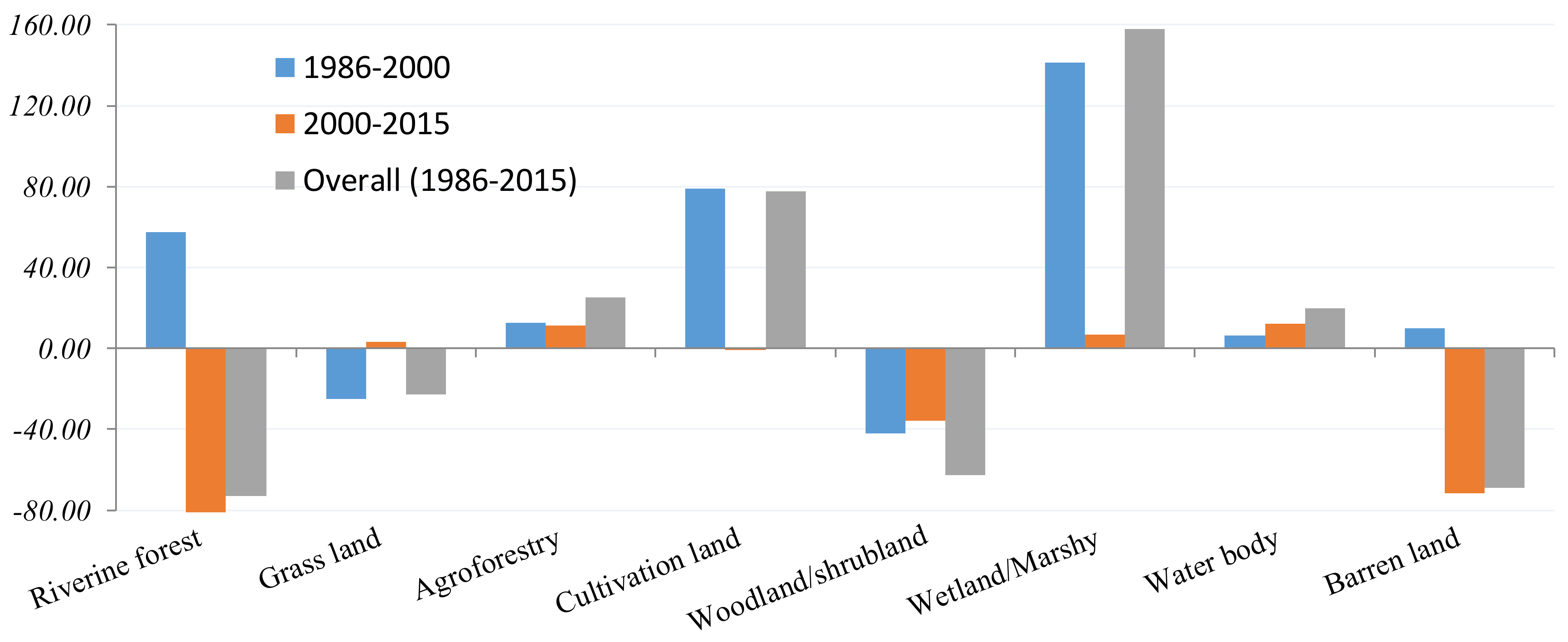
3.1. Land Use/Cover Change

Figure 3 depicts the LUC changes in Gedeo–Abaya landscape for the period 1986–2015. Agroforestry appears to be the dominant class throughout the study period, eventually increasing by 25.1% in 2015. The largest and rapid spatial reduction was for woodland/shrubland (62.8%), with an annual change rate of −3.7%, followed by grassland. Wetland/marshes increased threefold (158.1%), with a +6% annual change rate, followed by agroforestry and cultivation land. Agroforestry is the dominant class in the upstream landscape, while grazing land, woodland/shrubland, and wetlands are the dominant classes downstream. Commercially cultivated land has emerged only in the most recent decade downstream. As detailed by Temesgen et al. [37], woodland/shrubland cover was significantly cleared to introduce large-scale agribusiness farms downstream. Generally, natural vegetation classes (woodland, grassland, and riverine forest) showed significant reduction right through the study period (Figure 3, Table 1).

3.2. Estimation of Changes in ESs

Using our own VCs (Table 3) and the area covered by each LUC class (Table 1), an ESV for each cover category and the total value for each study year (1986, 2000, and 2015) were calculated. In 1986, agroforestry ($36.2 million/year ≈ 28.0%), woodland/shrubland ($34.7 million/year ≈ 26.9%), grassland ($20.0 million/year ≈ 15.5%) and wetland/marshes ($19.5 million/year ≈ 15.1%) were the dominant classes providing services. In 2000, wetland/marshes lead the service provision followed by agroforestry, woodland/shrubland, and grassland. The aggregate ESV for these leading land uses accounted for about 84.8%, indicating that these categories provide the most important ESs in the Gedeo–Abaya landscape.
A similar service provision trend continued from 2000 to 2015, except that woodland/shrubland’s service provision continually dropped and ranked fifth, being overtaken by that of water bodies. The sudden fall of woodland/shrub coverage and its ES share is attributed to the emergence of commercial agriculture following extensive investment downstream since 2007/2008 [37].
Our study area experienced a $18.3 million (over 14.2%) net increment in ESV from 1986 to 2015 (Table 5). The predominant cover, agroforestry, accounted for nearly 40.5% of the total study area and 30.7% of the total ESV in 2015. Similarly, a threefold increase, from 3.7% in 1986 to 8.9% coverage of the total study area in 2015, was computed for wetland/marshes. With such a small cover share, it accounted for 15.1% ($19.5 million) in 1986 and 34.2% ($50.4 million) of the total ESV in 2015. Together with agroforestry, these values cover 64.9% of the total service value share of the landscape ES at the final study period (Figure 4). Although the ESVs of most natural vegetation classes were considerably reduced (Table 5), the reductions were too small to counterbalance increases of the agroforestry and wetland classes, the areas and/or ESVs of which were too high to be offset.

3.3. General Trends in the Services of Individual Ecosystem Functions

The overall trends in ESV of individual ecosystem functions (ESVf) for each study period, and their overall changes, were calculated (Table S1, Supplementary Data). In 1986, habitats/refugia, climate regulation, food supply, water supply, and erosion control were among the dominant service function types in that order, accounting for 73.5% of the total value in the landscape. As shown in Table 1, woodland destruction was prominent right through the study period which has had a direct impact on habitat/refugia services to be dropped in 2015. As a result, food supply led the service provision followed by water supply, erosion control, and climate regulation. With apparently equal contributions, service functions in regulating and supporting service categories had the largest share. Given the steep and rugged topography of most part of the study landscape, particularly upstream, the ES function estimated for erosion control is convincing (Table S1). The fact that most land uses are either natural vegetation type or agroforestry may imply the adaptions that the residents made to cope with the rugged topographic settings, particularly erosion control. Also important is that cultivated land appears to be less favored (with only 15.04% cover share in 2015), as it puts the study area under high erosion risk.
Similarly, significant overall changes were observed on the aggregate value changes of each service function to service categories. In 1986, regulating services ($50.2 million ≈ 38.9%) accounted for the largest annual share of total ESV, followed by provisioning services ($49.2 million ≈ 38.2%). In 2015, both regulating and supporting services sharply increased, to $60.0 million and $57.9 million, respectively, reaching 80.0% of the total ESV. As can be seen in Table S1, changes in the contribution of each ESVf to the total ESV during the study periods were much greater for a few individual services, while too small for most of the rest. Only habitat, raw materials, and climate regulation services showed a slightly declining trend.

3.4. Relation between LUC Change and ES

Table 5 and Figure 4 depict the flow of LUC change impact on the necessary supplies of various ES. Downstream, the reduction of natural vegetation classes (Figure 4) led to a threefold expansion of wetland/marshes, which in turn increased the overall economic values of individual service function types and the entire ESV. Of all individual service function types, habitat, raw materials, and climate regulation services show a declining trend, which might also be attributed to woodland destruction for charcoaling and agribusiness. In contrast, the rejuvenation trend upstream enhanced the expansion of agroforestry, due largely to cultivation, grazing, and barren fields in the semiarid agropastoral region [37], and hence contributed to the net increase in total ESV.

3.5. Ecosystem Services Sensitivity Analyses

As in several previous works [32,49,55], we considered the effects of using alternative coefficients to estimate total ESV in our study landscape. Using Equation (4), we calculated coefficients of sensitivity, (CS) with a 50% adjustment in the service value coefficient for selected LUC classes, as shown in Table 6. Table 6 also shows the SEM that was calculated to indicate the uncertainty with the estimates of the mean values so as to compare with CS values. As discussed in Section 2.3, a reasonably low sensitivity of ESVs to changes in the VCs (that is, CS < 1) should be attained for the results of our analysis to be dependable. In all cases, the computed CS results were less than one, indicating the relative low sensitivity (inelasticity) of the landscape’s estimated total ESV with respect to own developed VCs. The highest CS was registered for those dominant LUC classes covering large shares of the total landscape and/or having high value coefficients (CS ≈ 0.15–0.34 for wetland/marshes and 0.28–0.31 for agroforestry). It is also important to mention that mean ± SEM values appear to be close to VC ± 50%, except for services provided from the agroforestry LUC. As a whole, the sensitivity analysis results indicate that our estimates for the studied area were robust, regardless of uncertainties in the VCs.

3.6. Land Use and Conservation Policy Implications of ESV Trends

Expansions of agroforestry and wetland covers ensured a net gain of 14.2% ESV in the study area (Table 5). Several contributing factors identified by zonal and local administrators include the variability resistance of agroforests to recurrent drought/rainfall as compared to monocropping, the increased interest of agropastoral farmers in adopting coffee and enset crops (the building blocks of the area’s agroforestry system), a government-led land rehabilitation campaign, and the formulation and implementation of regional land use and land administration policy [37]. During our field work, we realized that the latter two factors are actively in progress within the community and the local government offices.
Although its current efficiency and future sustainability require scientific witness, the government has made great efforts to improve land use management in the last two decades [56]. The responsible sector(s) mobilized farmers and sector experts with the local community for annual land rehabilitation campaigns, enclosure deals, and implementations on degraded areas. Recurrent work through safety net programs was also conducted and strongly supported the campaigns [56,57,58]. It is likely that community land use preference and government policies and implementation commitments have both contributed to the relative ecological betterment of the landscape. However, much has to be done to improve land use productivity upstream (see also [23,24]) and to address downstream changes with an eye to societal benefits.

4. Discussion

Since most ESs are not traded in markets and need to be valued using intricate non-market pricing techniques, more indirect and varied means of valuation must be devised and used frequently. Each valuation methodology has its own strengths and limitations which then restrict its use on the type of ecosystems, the services to be valued, and the information available to valuate [10]. Being aware of the limitations with BT, our approach increases the number of values to be sourced (Table 3) via established value sourcing tools (Figure 2) for the sake of accuracy of the averaged value transfer. Similarly, our attempt of estimating natural capital still has limitations that arise from overlap of ecosystem services and service categories, leading to the likely presence of economic double-counting in the final value estimation. According to MEA ([4], p. 35), this problem persists due to the interdependence of ecological values particularly between supporting services (whose services are not directly used by the people) and the other three service bundles. In our method, we have attempted to separately calculate service values for each category that using more services simultaneously [8]. Yet, we feel that the double-counting problem is not well managed and hence more dynamic models that can take account of the interdependencies between services of various service categories need to be developed.
More than 120 values were sourced, mainly from ESVD [52], to establish VCs for our study landscape. Through BT, our approach of employing LUC datasets as a proxy of measurement facilitated the ESV estimation process. Based on the procedures that followed, we believe that we developed a conservative and locally valid model. In principle and practice, the exercise of valuing natural capital considers minimum service values, mainly because of uncertainties and variation of valuation techniques [47]; the complex, dynamic, and nonlinear properties of ecosystems [59]; and other circumstances, like ecosystem infrastructures, which have a significant role in maximizing ESV [8,34]. In our case, water bodies are a good example. For instance, our VC for the class ‘water body’ (Table 3), which mainly means the northeastern part of Lake Abaya ($3,226.8/ha/year in 2007 US$) is much less than the VC of Kindu et al. [32] for Lake Langano ($8103.5/ha/year with 1994 US$). The ecosystem infrastructure of Lake Abaya is far poorer than that of Lake Langano, which is situated close to the capital and is one of the country’s popular recreational lakes. Similarly, our wetland/marshes VC is much less than those estimations of Costanza et al. [8] and De Groot et al. [9] for global inland wetland biomes (Table 2). These examples should indicate the probability of our minimizing estimates of economic valuation of ES when using modified VC instead of using global values.
Based on the estimated sizes of land use categories and using our own locally developed ecosystem services VCs for related biomes, we determined the values of individual ecosystem service functions and the total annual service values. Our results clearly show agroforestry and wetland/marshes as the predominant, and continually expanding, classes while natural vegetation classes are declining (Figure 5d). The predominance of agroforestry cover and the high VC of wetland/marshes dominated the landscape’s total ESV and led to a $18.3 million net increase in ES, a comparative reflection of overall ecological/ecosystem resilience in our study landscape. Perhaps this is not a common result in the tropics. In the highlands of Ethiopia, Tolessa et al. [55] calculated a net loss of $3.7 million ESV for Chillimo forest using Costanza et al.’s global VC, while Kindu et al. [32] estimated a $45.9 million loss using the same method; the latter fell to $19.3 million when the researchers’ own modified VC was used.
Two major acts in the nation’s land use and management perspectives could primarily be credited for the increasing trend of Gedeo–Abaya net ESV: governmental attention to land resources management through the annual land rehabilitation campaign of more than a decade; and the sustainable farming culture of the community, particularly upstream. We view the latter as the more important factor. These factors can also be seen in Ethiopia’s decades of natural resources management along with political/institutional transitions through 1986–2015. The first decade saw destruction of vast ecosystems due to unbridled civil war between the military government and its opponents, which eventually ended in 1991, followed by a transition period to the new government. Similar devastating effects of civil war and societal unrest are commonly noted by researchers elsewhere in the tropics (see for example References [37,60]). In the second decade, the current government, the Federal Democratic Republic of Ethiopia, established itself and started to consider and act on natural resource conservation policies and institutions and their implementations. During the third decade, extensive work was conducted and meaningful achievements recorded, especially in northern Ethiopia [37,56,58].
As discussed above, LUC can be used as a proxy for ES, but the biomes used as proxies are not always perfect matches [10,49]. Similar ecosystem complexity, environmental, and socioeconomic circumstances increase the ability to match the study site and policy site during value transfer. Furthermore, economic valuation studies are generally absent for distinctive traditional agroforestry ecosystems; these factors are among the challenges to ESV assignment to LUC class. In southern Ethiopia, agroforests are modifications of natural forests to maximize forest coffee productivity; hence, they demonstrate that “agroforestry is an ancient agricultural form of forest land management” [12]. As examined by Negash and Achalu [21], Gedeo’s traditional agroforestry was originally dominated by naturally grown tree species, which still constituted 90% of the area’s trees. They also found that upper-story plant species (the forest component) in the system occupied 38% of the vertical strata. Depending on this figure, we assumed the minimum share of the forest component of Gedeo’s agroforests to be 35%, with the rest 60% perennial crops/shrubs/herbs and 5% annual crops. Following UNESCO [14] consensus that an agroforestry system can have protective, regulative and productive functions similar to forest ecosystems, the ESV estimation of tropical forests was partly used as a proxy, although some individual ESV functions (like cultural and cognitive development) should be much higher their current estimated values. However, the results of our sensitivity analysis suggest that, despite these acknowledged limitations, the approach we used can produce valuable results.

5. Conclusions

Our 1848 km2 area, with eight land use categories, yielded a total annual ESV of $129 × 106 in 1986 and $147 × 106 in 2015, a 14.2% increment in three decades. These figures show the relative resilience of the Gedeo–Abaya landscape; but losses were still experienced in natural vegetation classes whose area and VC were too small to offset their value increments due to the high economic value of expanded agroforestry and wetland/marshes. Agroforestry is the predominant class, despite its productivity challenges in recent years due to overpopulation. It is a dynamic ecologically based system which seeks to diversify and sustain production for increased socioeconomic and environmental benefits at all levels. Semi-natural forests, representing most agroforests, are the source of all livelihood of quite large local populations. Understanding these unique features, we strongly recommend the economic value of agroforests be studied as a separate biome at large scales.
From a decision-making standpoint, it is critical to distinguish invaluable ecosystems that (1) deliver high economic value and (2) contribute to increased cumulative ESV. Both scenarios require appropriate interventions to minimize the negative impacts of ongoing destruction while maintaining the others.
Keeping in mind the persisting caveats regarding valuation of ES in monetary units, these estimates are ever more important: not only to the economic valuation of ES and in considering these services during decision making processes, but also for the study of and improvements to projects in other similar agroecological settings. It is also important for appraisal of socio-cultural preferences with regard to ES to identify the impact of different management options on the societies and the service delivery capacities of ecosystems. Finally, the use of ES highlights the significance of socially beneficial ecological processes. Works of land use and policy making should aim at balancing society’s needs and preferences while sustaining ES, as natural ecosystems are preserved and used appropriately.

Supplementary Materials

The supplementary files are available online at https://www.mdpi.com/2071-1050/10/4/1126/s1.

Acknowledgments

The authors gratefully thank Dilla University for providing a vehicle for fieldwork. Their special thanks also go to Gedeo zone and Abaya woreda experts and the community for their insights and cooperation during the fieldwork as well as to Abiyot Legesse, Tadesse Jaleta and Ongaye Oda for editorial or/and technical support. The authors are also thankful to the National Nature Sciences Foundation of China (Fund No. 41571176) and the 111 Project (No. B17024) for financial support.

Author Contributions

The first author, Habtamu Temesgen, designed the research and wrote the paper. Wei Wu, Xiaoping Shi, Mengistie Kindu, Mengistie Kindu and Belewu Bekele contributed to the work through their persistent guidance editorial works. All authors read and approved the final manuscript.

Conflicts of Interest

The authors declare no conflict of interest.

References

  1. Daily, G. Nature’s Services: Societal Dependence on Natural Ecosystems; Island Press: Washington, DC, USA, 1997. [Google Scholar]
  2. Wang, Z.; Mao, D.; Li, L.; Jia, M.; Dong, Z.; Miao, Z.; Ren, C.; Song, C. Quantifying changes in multiple ecosystem services during 1992–2012 in the Sanjiang Plain of China. Sci. Total Environ. 2015, 514, 119–130. [Google Scholar] [CrossRef] [PubMed]
  3. De Groot, R.S.; Wilson, M.A.; Boumans, R.M. A typology for the classification, description and valuation of ecosystem functions, goods and services. Ecol. Econ. 2002, 41, 393–408. [Google Scholar] [CrossRef]
  4. MEA. Ecosystems and Human Well-Being: Wetlands and Water; World Resources Institute: Washington, DC, USA, 2005. [Google Scholar]
  5. FAO. Global Forest Resources Assessment 2015: How Have the World’s Forests Changed? FAO: Rome, Italy, 2015. [Google Scholar]
  6. Sloan, S.; Sayer, J.A. Forest Resources Assessment of 2015 shows positive global trends but forest loss and degradation persist in poor tropical countries. For. Ecol. Manag. 2015, 352, 134–145. [Google Scholar] [CrossRef]
  7. Brink, A.B.; Bodart, C.; Brodsky, L.; Defourney, P.; Ernst, C.; Donney, F.; Lupi, A.; Tuckova, K. Anthropogenic pressure in East Africa—Monitoring 20 years of land cover changes by means of medium resolution satellite data. Int. J. Appl. Earth Obs. Geoinf. 2014, 28, 60–69. [Google Scholar] [CrossRef]
  8. Costanza, R.; D’arge, R.; De Groot, R.; Farber, S.; Grasso, M.; Hannon, B.; Limburg, K.; Naeem, S.; O’neill, R.; Paruelo, J.; et al. The value of the world’s ecosystem services and natural capital. Nature 1997, 387, 253–260. [Google Scholar] [CrossRef]
  9. De Groot, R.; Brander, L.; Van Der Ploeg, S.; Costanza, R.; Bernard, F.; Braat, L.; Christie, M.; Crossman, N.; Ghermandi, A.; Hein, L. Global estimates of the value of ecosystems and their services in monetary units. Ecosyst. Serv. 2012, 1, 50–61. [Google Scholar] [CrossRef]
  10. Mendoza-González, G.; Martínez, M.; Lithgow, D.; Pérez-Maqueo, O.; Simonin, P. Land use change and its effects on the value of ecosystem services along the coast of the Gulf of Mexico. Ecol. Econ. 2012, 82, 23–32. [Google Scholar] [CrossRef]
  11. Yirsaw, E.; Wu, W.; Temesgen, H.; Bekele, B. Effect of temporal land use/land cover changes on ecosystem services value in coastal area of China: The case of Su-Xi-Chang region. Appl. Ecol. Environ. Res. 2016, 14, 409–422. [Google Scholar] [CrossRef]
  12. Casey, J.F. Agroforestry adoption in Mexico: Using Keynes to better understand farmer decision-making. J. Post Keynes. Econ. 2004, 26, 505–521. [Google Scholar]
  13. Wiersum, K. Forest gardens as an ‘intermediate’ land-use system in the nature-culture continuum: Characteristics and future potential. In New Vistas in Agroforestry; Springer: Dordrecht, The Netherlands, 2004. [Google Scholar]
  14. UNESCO. Tropical Forest Ecosystems. A State-Of-The Knowledge Report Prepared by UNESCO/UNEP/FAO; Natural Resources Research; UNESCO: Paris, France, 1987; Volume 14. [Google Scholar]
  15. Marjokorpi, A.; Ruokolainen, K. The role of traditional forest gardens in the conservation of tree species in West Kalimantan, Indonesia. Biodivers. Conserv. 2003, 12, 799–822. [Google Scholar] [CrossRef]
  16. Petit, L.J.; Petit, D.R. Evaluating the Importance of Human-Modified Lands for Neotropical Bird Conservation. Conserv. Biol. 2003, 17, 687–694. [Google Scholar] [CrossRef]
  17. Nair, P. The coming of age of agroforestry. J. Sci. Food Agric. 2007, 87, 1613–1619. [Google Scholar] [CrossRef]
  18. Noble, I.R.; Dirzo, R. Forests as human-dominated ecosystems. Science 1997, 277, 522–525. [Google Scholar] [CrossRef]
  19. Jose, S. Agroforestry for ecosystem services and environmental benefits: An overview. Agrofor. Syst. 2009, 76, 1–10. [Google Scholar] [CrossRef]
  20. Kanshie, T.K. Five Thousand Years of Sustainability? A Case Study on Gedeo Landuse (Southern Ethiopia); Citeseer: State College, PA, USA, 2002. [Google Scholar]
  21. Negash, M.; Achalu, N. History of Indigenous Agro-Forestry in Gedeo, Southern Ethiopia, Based on local community interviews: Vegetation diversity and structure in the Land-use systems. Ethiop. J. Nat. Resour. 2008, 10, 31–52. [Google Scholar]
  22. CSA. Population Projection of Ethiopia for All Regions at Wereda Level from 2014–2017; Central Statistical Authority: Addis Ababa, Ethiopia, 2013. [Google Scholar]
  23. Legesse, A. The Dynamics of Gedeo Agroforestry and Its Implications to Sustainability. Ph.D. Thesis, University of South Africa, Pretoria, South Africa, 2014. [Google Scholar]
  24. Negash, M.; Yirdaw, E.; Luukkanen, O. Potential of indigenous multistrata agroforests for maintaining native floristic diversity in the south-eastern Rift Valley escarpment, Ethiopia. Agrofor. Syst. 2012, 85, 9–28. [Google Scholar] [CrossRef]
  25. Dawoe, E.K.; Isaac, M.E.; Quashie-Sam, J. Litterfall and litter nutrient dynamics under cocoa ecosystems in lowland humid Ghana. Plant Soil 2010, 330, 55–64. [Google Scholar] [CrossRef]
  26. Starr, M.; Saarsalmi, A.; Hokkanen, T.; Merilä, P.; Helmisaari, H.S. Models of litterfall production for Scots pine (Pinus sylvestris L.) in Finland using stand, site and climate factors. For. Ecol. Manag. 2005, 205, 215–225. [Google Scholar] [CrossRef]
  27. Nair, P.; Garrity, D. Agroforestry, the Future of Global Land Use; Nair, P.K.R., Garrity, D., Eds.; Springer: Dordrecht, The Netherlands, 2012. [Google Scholar]
  28. Debelo, A.R.; Legesse, A.; Milstein, T.; Orkaydo, O.O. “Tree is life”: The rising of Dualism and the Declining of Mutualism among the Gedeo of southern Ethiopia. Front. Commun. 2017, 2, 7. [Google Scholar] [CrossRef]
  29. Bevan, P.; Pankhrust, A. Ethiopian Villages Studies: Adado Gedeo. 1996. Available online: http://ethiopiawide.net/wp-content/uploads/adado1995 (accessed on 12 May 2005).
  30. Tadesse, G.; Zavaleta, E.; Shennan, C.; Fitzsimmons, M. Local Ecosystem Service Use and Assessment Vary with Socio-ecological Conditions: A Case of Native Coffee-Forests in Southwestern Ethiopia. Hum. Ecol. 2014, 42, 873–883. [Google Scholar] [CrossRef]
  31. Bishaw, B.; Neufeldt, H.; Mowo, J.; Abdelkadir, A.; Muriuki, J.; Dalle, G.; Assefa, T.; Guillozet, K.; Kassa, H.; Dawson, I.K. Farmers’ Strategies for Adapting to and Mitigating Climate Variability and Change through Agroforestry in Ethiopia and Kenya; Forestry Communications Group, Oregon State University: Corvallis, OR, USA, 2013. [Google Scholar]
  32. Kindu, M.; Schneider, T.; Teketay, D.; Knoke, T. Changes of ecosystem service values in response to land use/land cover dynamics in Munessa-Shashemene landscape of the Ethiopian highlands. Sci. Total Environ. 2016, 547, 137–147. [Google Scholar] [CrossRef] [PubMed]
  33. Yaron, G. Forest, plantation crops or small-scale agriculture? An economic analysis of alternative land use options in the Mount Cameroon area. J. Environ. Plan. Manag. 2001, 44, 85–108. [Google Scholar] [CrossRef]
  34. Turner, R.K.; Pearce, D.W. Sustainable economic development: Economic and ethical principles. In Economics and Ecology; Springer: Dordrecht, The Netherlands, 1993. [Google Scholar]
  35. Negasa, T.; Ketema, H.; Legesse, A.; Sisay, M.; Temesgen, H. Variation in soil properties under different land use types managed by smallholder farmers along the toposequence in southern Ethiopia. Geoderma 2017, 290, 40–50. [Google Scholar] [CrossRef]
  36. Mebrate, B.T. Agroforestry Practices in Gedeo Zone Ethiopia a Geographical Analysis. Ph.D. Thesis, Panjab University, Chandigarh, India, 2007. [Google Scholar]
  37. Temesgen, H.; Wu, W.; Legesse, A.; Yirsaw, E.; Bekele, B. Landscape based upstream-downstream prevalence of land use/cover change drivers in southeastern rift escarpment of Ethiopia. Environ. Monit. Assess. 2018, 190, 166. [Google Scholar] [CrossRef] [PubMed]
  38. Bottomley, B. Mapping Rural Land Use & Land Cover Change in Carroll County, Arkansas Utilizing Multi-Temporal Landsat Thematic Mapper Satellite Imagery; University of Arkansas: Fayetteville, AR, USA, 1998. [Google Scholar]
  39. Jensen, J.R. Remote Sensing of the Environment: An Earth Resource Perspective 2/e; Pearson Education India: Kerala, India, 2009. [Google Scholar]
  40. Lillesand, T.; Kiefer, R.; Chipman, J. Remote Sensing and Image Analysis; John Wiley and Sons: New York, NY, USA, 2000. [Google Scholar]
  41. TEEB Foundations. The Economics of Ecosystems and Biodiversity: Ecologicaland Economic Foundations; Kumar, P., Ed.; Earthscan: London, UK; Washington, DC, USA, 2010. [Google Scholar]
  42. Liu, S.; Costanza, R.; Farber, S.; Troy, A. Valuing ecosystem services. Ann. N. Y. Acad. Sci. 2010, 1185, 54–78. [Google Scholar] [CrossRef] [PubMed]
  43. Costanza, R.; De Groot, R.; Sutton, P.; Van Der Ploeg, S.; Anderson, S.J.; Kubiszewski, I.; Farber, S.; Turner, R.K. Changes in the global value of ecosystem services. Glob. Environ. Chang. 2014, 26, 152–158. [Google Scholar] [CrossRef]
  44. Xie, G.-D.; Lu, C.-X.; Leng, Y.-F.; Zheng, D.; Li, S. Ecological assets valuation of the Tibetan Plateau. J. Nat. Resour. 2003, 18, 189–196. [Google Scholar]
  45. Johnston, R.J.; Rolfe, J.; Rosenberger, R.S.; Brouwer, R. Benefit Transfer of Environmental and Resource Values; Springer: Dordrecht, The Netherlands, 2015. [Google Scholar]
  46. Nelson, E.; Mendoza, G.; Regetz, J.; Polasky, S.; Tallis, H.; Cameron, D.; Chan, K.; Daily, G.C.; Goldstein, J.; Kareiva, P.M. Modeling multiple ecosystem services, biodiversity conservation, commodity production, and tradeoffs at landscape scales. Front. Ecol. Environ. 2009, 7, 4–11. [Google Scholar] [CrossRef]
  47. Rosenberger, R.S.; Stanley, T.D. Measurement, generalization, and publication: Sources of error in benefit transfers and their management. Ecol. Econ. 2006, 60, 372–378. [Google Scholar] [CrossRef]
  48. Wilson, M.A.; Hoehn, J.P. Valuing environmental goods and services using benefit transfer: The state-of-the art and science. Ecol. Econ. 2006, 60, 335–342. [Google Scholar] [CrossRef]
  49. Kreuter, U.P.; Harris, H.G.; Matlock, M.D.; Lacey, R.E. Change in ecosystem service values in the San Antonio area, Texas. Ecol. Econ. 2001, 39, 333–346. [Google Scholar] [CrossRef]
  50. Brouwer, R. Environmental value transfer: State of the art and future prospects. Ecol. Econ. 2000, 32, 137–152. [Google Scholar] [CrossRef]
  51. Navrud, S.; Ready, R. Review of methods for value transfer. In Environmental Value Transfer: Issues and Methods; Springer: Dordrecht, The Netherlands, 2007; pp. 1–10. [Google Scholar]
  52. Van Der Ploeg, S.; De Groot, R. The TEEB Valuation Database—A Searchable Database of 1310 Estimates of Monetary Values of Ecosystem Services; Foundation for Sustainable Development: Wageningen, The Netherlands, 2010. [Google Scholar]
  53. DEFRA. An Introductory Guide to Valuing Ecosystem Services; Defra Publications: London, UK, 2007; 66p.
  54. Kubiszewski, I.; Costanza, R.; Dorji, L.; Thoennes, P.; Tshering, K. An initial estimate of the value of ecosystem services in Bhutan. Ecosyst. Serv. 2013, 3, e11–e21. [Google Scholar] [CrossRef]
  55. Tolessa, T.; Senbeta, F.; Kidane, M. The impact of land use/land cover change on ecosystem services in the central highlands of Ethiopia. Ecosyst. Serv. 2017, 23, 47–54. [Google Scholar] [CrossRef]
  56. Adimassu, Z.; Langan, S.; Johnston, R. Understanding determinants of farmers’ investments in sustainable land management practices in Ethiopia: Review and synthesis. Environ. Dev. Sustain. 2016, 18, 1005–1023. [Google Scholar] [CrossRef]
  57. Beyene, F. Land use change and determinants of land management: Experience of pastoral and agro-pastoral herders in eastern Ethiopia. J. Arid Environ. 2016, 125, 56–63. [Google Scholar] [CrossRef]
  58. Wolancho, K.W. Evaluating watershed management activities of campaign work in Southern nations, nationalities and peoples’ regional state of Ethiopia. Environ. Syst. Res. 2015, 4, 6. [Google Scholar] [CrossRef]
  59. Turner, R.K.; Paavola, J.; Cooper, P.; Farber, S.; Jessamy, V.; Georgiou, S. Valuing nature: Lessons learned and future research directions. Ecol. Econ. 2003, 46, 493–510. [Google Scholar] [CrossRef]
  60. Tsegaye, D.; Moe, S.R.; Vedeld, P.; Aynekulu, E. Land-use/cover dynamics in Northern Afar rangelands, Ethiopia. Agric. Ecosyst. Environ. 2010, 139, 174–180. [Google Scholar] [CrossRef]
Figure 1. Study area map showing agroecological settings (from 1104 to 3005 m a.s.l) of the studied landscape.
Sustainability 10 01126 g001
Figure 2. Schematic methodological flow.
Sustainability 10 01126 g002
Figure 3. Land use/cover change between periods (%) of the Gedeo–Abaya landscape (calculated as 100 × (A final year − A initial year)/A initial year, where A = area of the LUC type).
Sustainability 10 01126 g003
Figure 4. Contributing percentages of area and ESV for each LUC category in each study period.
Sustainability 10 01126 g004
Figure 5. Some pictorial representations of land uses and their challenges in the Gedeo-Abaya landscape: (a) the agroforestry belt on a steeply and rugged topography; (b) a semi-natural forest appearance of agroforestry systems; (c) utilization of the tree component which is affecting system productivity; (d) woodland destruction downstream; (e) the pastoral life, showing cattle’s population impact on natural vegetation cover; and (f) expanding wetland to grassland area with multipurpose ESs. All photos are by the first author except (c), which is reproduced with permission from a field report of “Friends of the Gedeo Agroforestry system” urging registration as a UNESCO World Heritage Site in 2009.
Sustainability 10 01126 g005
Table 1. Estimated area (ha) of land use/cover (LUC) change in the Gedeo–Abaya landscape and overall change (%) between periods, 1986–2015 [37].
LUC Type1986 (ha)%2000 (ha)%2015 (ha)%Overall Change (%) 1986–2015 *
Riverine forest543.70.29855.40.46147.70.08−72.83
Agroforestry59,828.232.3867,287.036.4174,856.040.5125.12
Woodland/shrubland38,687.020.9422,382.012.1114,383.07.78−62.82
Grassland56,286.430.4642,254.022.8743,582.023.58−22.57
Cultivation land15,633.38.4627,995.015.1527,791.015.0477.77
Barren land2211.51.202436.01.32686.70.37−68.95
Wetland/Marshes6836.23.7016,508.08.9317,641.09.55158.05
Water body4768.12.585077.02.755707.03.0919.69
Total184,794.4100184,794.4100184,794.4100
* Cover change between periods was calculated as 100 × (A final year − A initial year)/A initial year, where A = area of the LUC type.
Table 2. Descriptions of the LUC classes mapped in the area over the three study periods and summary of their respective ecosystem service valuation coefficients (VC) developed locally and globally by various authors. For our own VC, as shown in Table 3, GDP deflators, consumer price index, and producers price index were used to adjust to 2007 US$.
LUC TypeDescriptionEquivalent BiomeGlobal VCLocal VC
1994 $/ha/year [8]2007 $/ha/year [9]1994 $/ha/year [32]2007 $/ha/year (Our Own VC, Table 3)
Riverine forestA broad leaved tree along river courseTropical forest20085264986.71093.2
AgroforestryIntensively managed semi-natural forest area in which annual/perennial crops &/or animals deliberately used on the same land-management unitsTropical forest 604.4
Woodland/shrublandWoody Acacia dominated areas; also includes shrubland covered with small trees & bushes Woodland 1588 897.0
Tropical forest2008 986.7
GrasslandsGrass & herb cover with scattered trees and shrubsGrasslands2442871293.3355.5
Cultivation landCropping fields owned by small holder farmers and medium to large-scale investorsCrop land92 225.6169.2
Barren landBad areas and rook outcrops Desert0 00
Wetland/MarshyRiver beds, intermittent ponds and marshy areas with shallow water and permanent reed vegetationsInland Wetland14,78525,682 2856.1
Water bodyMainly refers to part of Abaya LakeFresh water849842678103.53226.8
Table 3. Monetary values for each ecosystem services per biome in $/ha/year (standardized values in 2007 US$).
Ecosystem ServicesLUC Types/Biome
Riverine ForestAgroforestryWoodland/ShrublandGrass LandCultivation LandWetland/MarshyWater Body
Provisioning services159.8172.3187.4183.4125.2813.12881.4
Food4.8102.811.7158.1125.2180.2157.5
Water46.016.120.9 257.02723.9
Raw material13.519.3130.324.3 209.0
Genetic resources94.032.924.50.0 68.4
Medical services1.51.1 1.0 98.5
Regulating services733.4358.0244.5166.627.01122.8309.3
Water regulation6.82.445.0 741.9
Water treatment56.019.6 33.0309.3
Erosion control523.9183.4104.0 81.3
Climate regulation132.5132.395.0143.3 199.3
Biological control14.36.30.5 27.0
Air quality regulation 14.0 23.3 67.4
Supporting services190.067.3459.30.017.0833.40.0
Nutrient cycling92.232.3 102.5
Pollination51.018.719.0 17.0
Soil formation18.66.510.0 43.5
Habitat/refugia28.29.9430.3 687.4
Cultural services10.06.85.95.50.086.736.2
Recreation8.06.15.95.5 20.736.2
Cultural2.00.7 66.0
Total economic ESV1093.2604.4897.0355.5169.22856.13226.8
Table 4. Descriptive statistics (mean, standard error, and standard deviation) of the total service values (in $×106 year–1 in 2007 US$) of ecosystem services per LUC types.
Services Total (N = 123)
No. of EstimatesTotal Service Mean ValuesStandard Error of the Mean (SEM)Standard Deviation (SD)
Riverine Forest341093.245.34264.38
Agroforestry a-604.412.7452.52
Woodland/Shrubland23897.053.85263.82
Grassland14355.527.58103.18
Cultivated land6169.227.1566.50
Wetland/Marshes382856.165.62376.98
Water body83226.86.641879.32
a Already counted under Riverine forest, Grassland or/and Cultivation land classes.
Table 5. Total ecosystem service valuation (ESV) (in $×106 year–1 in 2007 US$) estimated for each LUC type using our estimation model and area covered by each class.
LUC TypeESV ($×106/year)2000–19862015–2000Overall Change
198620002015$×106 year–1$×106 year–1$×106 year–1
Riverine forest0.59 (0.5%)0.94 (0.6%)0.16 (0.1%)0.34 (2.1%)−0.77 (−33.2%)−0.43 (−2.37%)
Agroforestry36.16 (28.0%)40.67 (28.1%)45.24 (30.7%)4.51 (28.3%)4.57 (196.2%)9.08 (49.69%)
Woodland/shrubland34.70 (26.9%)20.08 (13.8%)12.90 (8.8%)−14.63 (−91.7%)−7.18 (−307.7%)−21.80 (−119.28%)
Grass land20.01 (15.5%)15.02 (10.4%)15.49 (10.5%)−4.99 (−31.3%)0.47 (20.2%)−4.52 (−24.71%)
Cultivated land2.64 (2.0%)4.74 (3.3%)4.70 (3.2%)2.09 (13.1%)−0.03 (−1.5%)2.06 (11.25%)
Barren land0.000.000.000.000.000.00
Wetland/Marshy19.52 (15.1%)47.15 (32.5%)50.38 (34.2%)27.62 (173.2%)3.24 (138.8%)30.86 (168.84%)
Water body15.39 (11.9%)16.38 (11.3%)18.42 (12.5%)1.00 (6.3%)2.03 (87.2%)3.03 (16.58%)
Total129.0145.0147.315.95 (100%)2.33 (100%)18.28 (100%)
Note: Percentages of ESV for ecosystem service functions were parenthesized.
Table 6. Estimated total ecosystem service values (ESV in $×106) in the Gedeo–Abaya landscape after adjustment of own modified conservative service valuation coefficients (VC), the magnitude of changes in the ESV following the adjustments, and the CS associated with these adjustments. For value comparison, standard errors of the means (SEM) of VCs are also indicated.
Change in VCESV Adjusted aEffect of Changing VC from Original Value aTotal Service Mean ± SEM of Each VC
198620002015198620002015
%CS%CS%CS
Agroforestry VC ± 50%147.1165.3169.914.00.314.00.315.40.3604.4 ± 12.7
Woodland/shrubland VC ± 50%146.4155.0153.813.40.36.90.14.40.1897.0 ± 53.9
Grass land VC ± 50%139.0152.5155.07.80.25.20.15.30.1355.5 ± 27.6
Wetland/Marshy VC ± 50%138.8168.5172.57.60.216.30.317.10.32856.1 ± 65.6
a Using the formula: %ESV change = (ESVfinal year − ESVinitial year)/ESVinitial year × 100.

