Energy Cost Optimization for Water Distribution Networks Using Demand Pattern and Storage Facilities

Abstract
1. Introduction
2. Materials and Methods
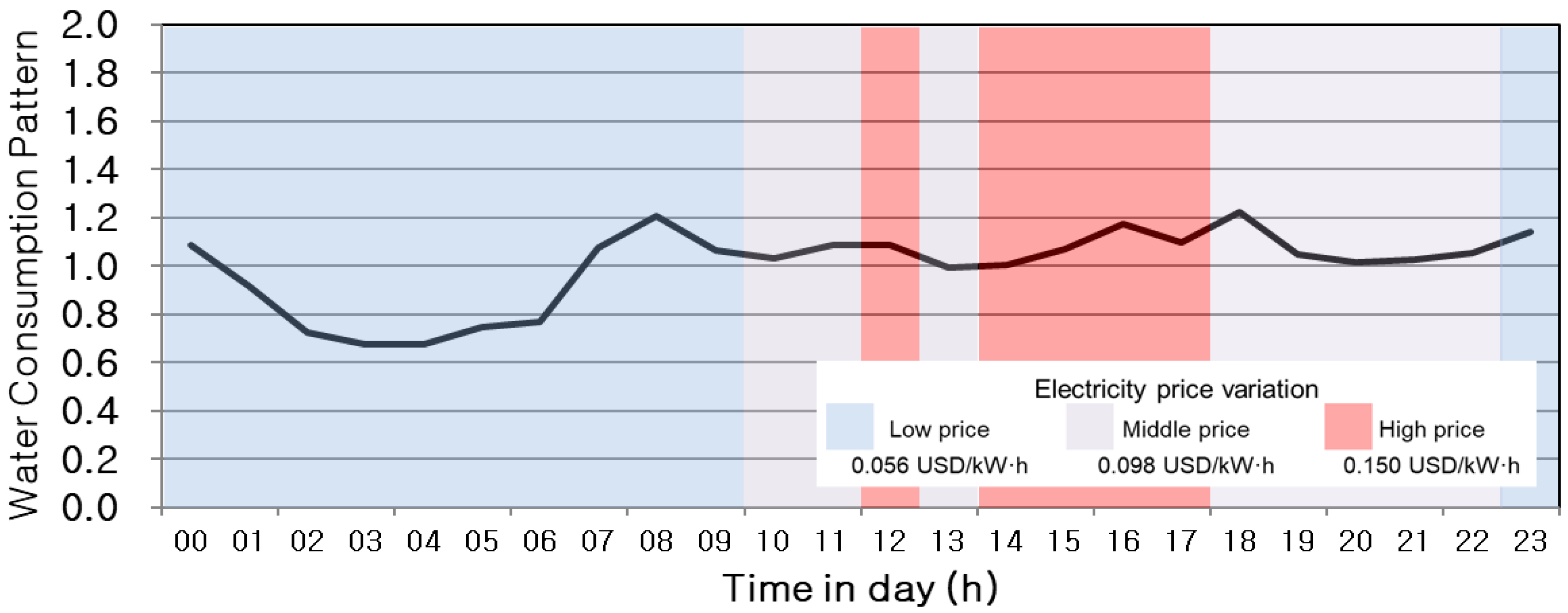
2.1. Energy Consumption
2.2. Water Storage Facilities
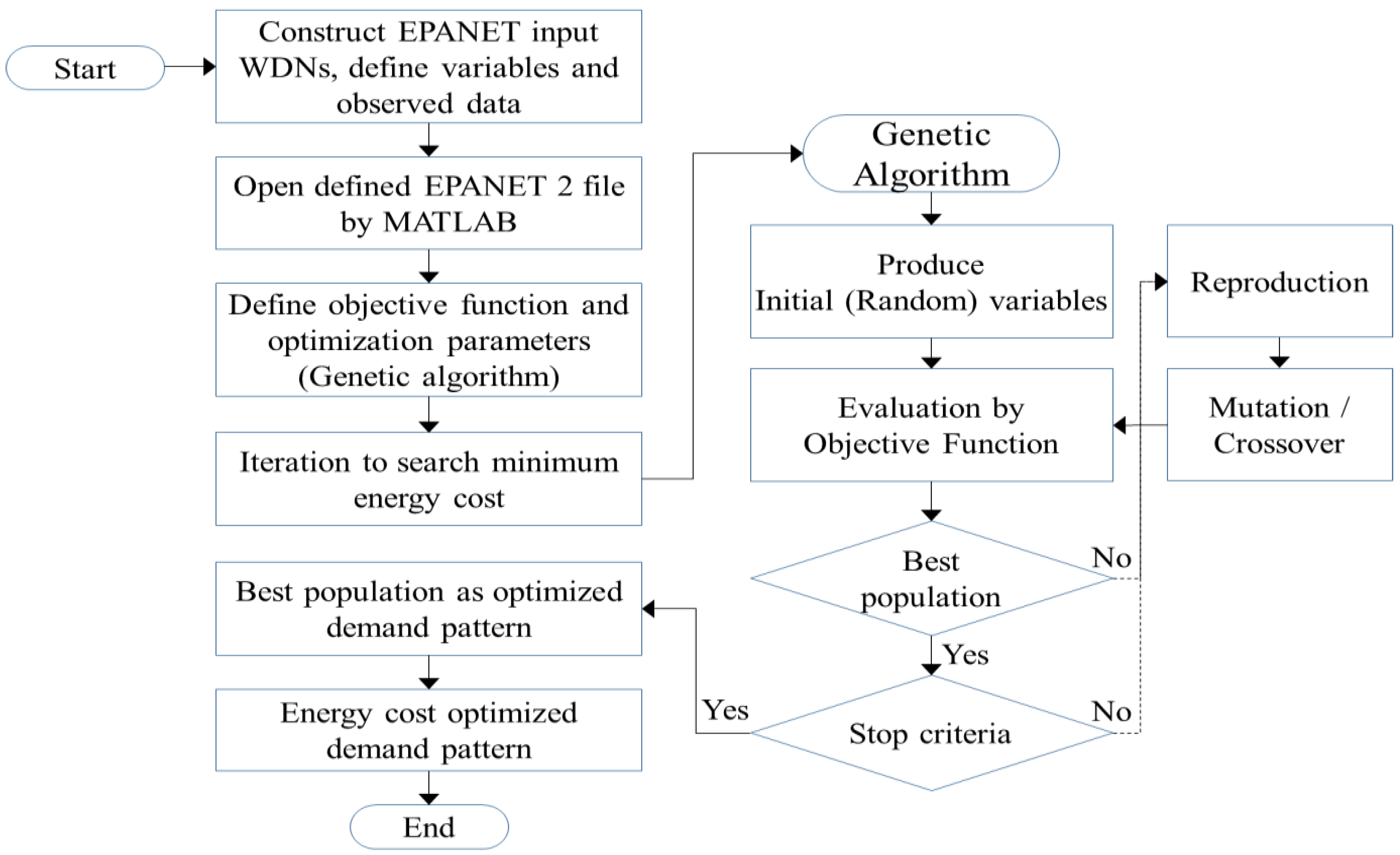
2.3. EPANET
2.4. Genetic Algorithms
3. Development of the Optimization Tool
3.1. Objective Function
3.2. Study Area
4. Results and Discussion
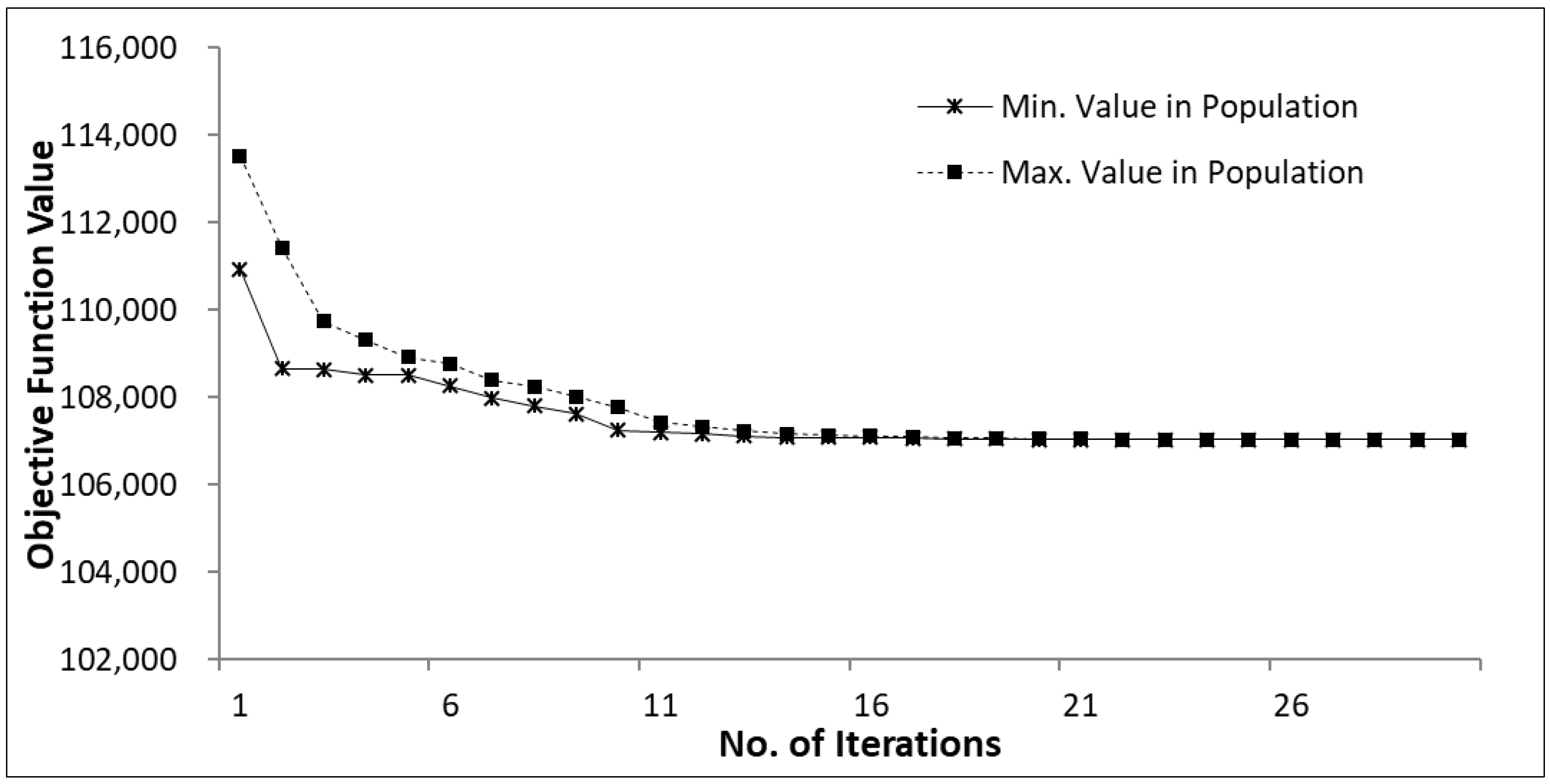
4.1. Model Sensitivity and Convergence
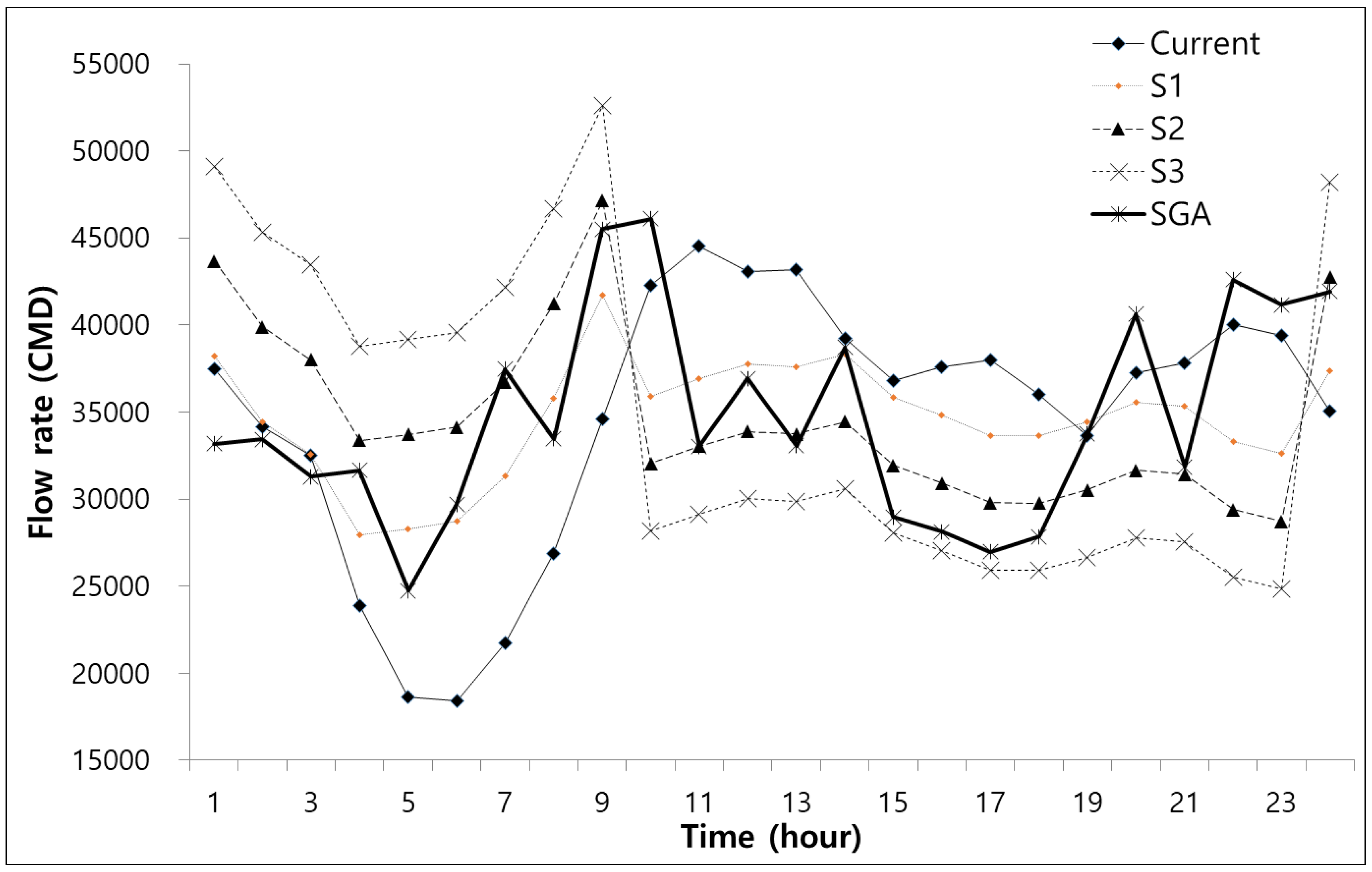
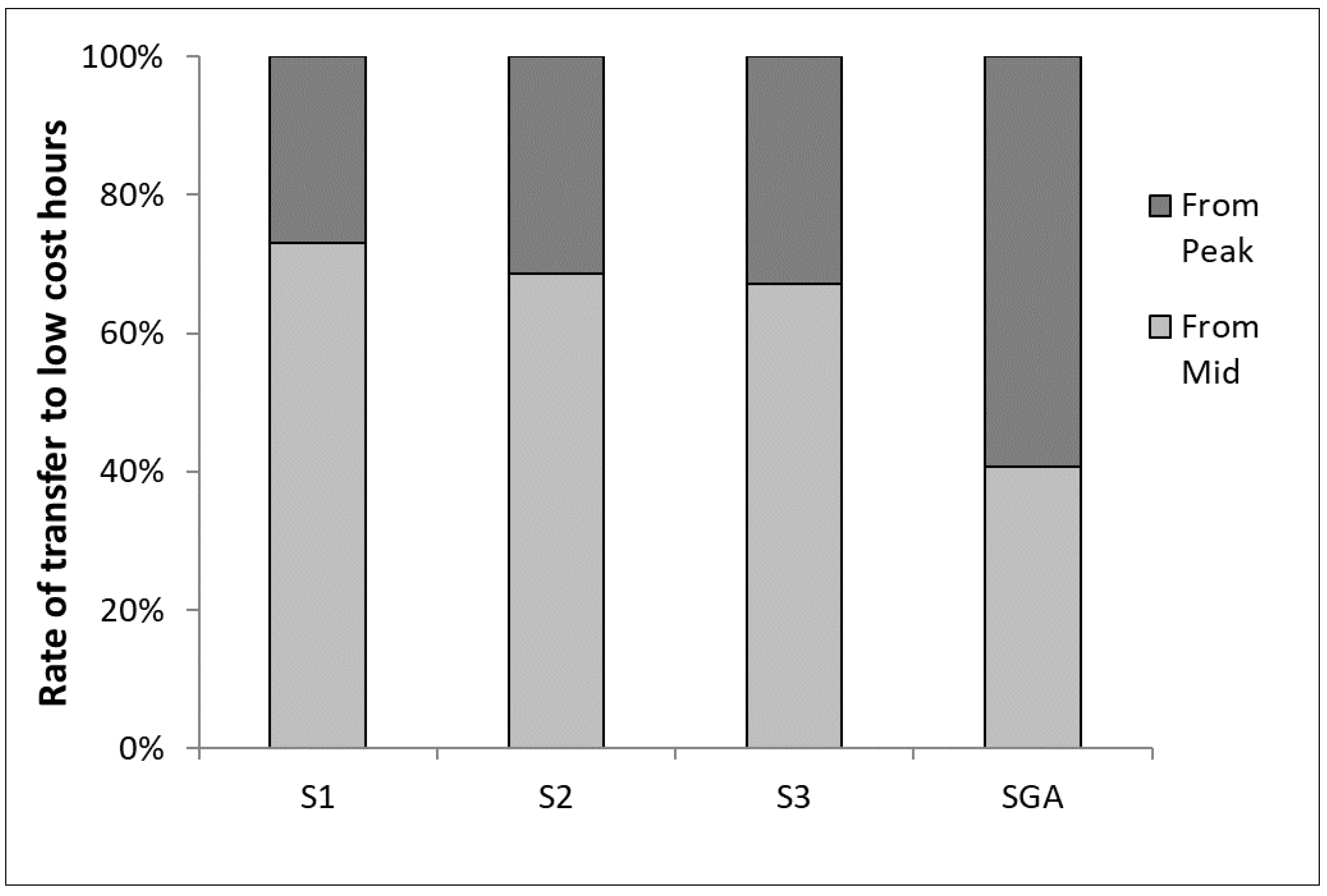
4.2. Summer Season
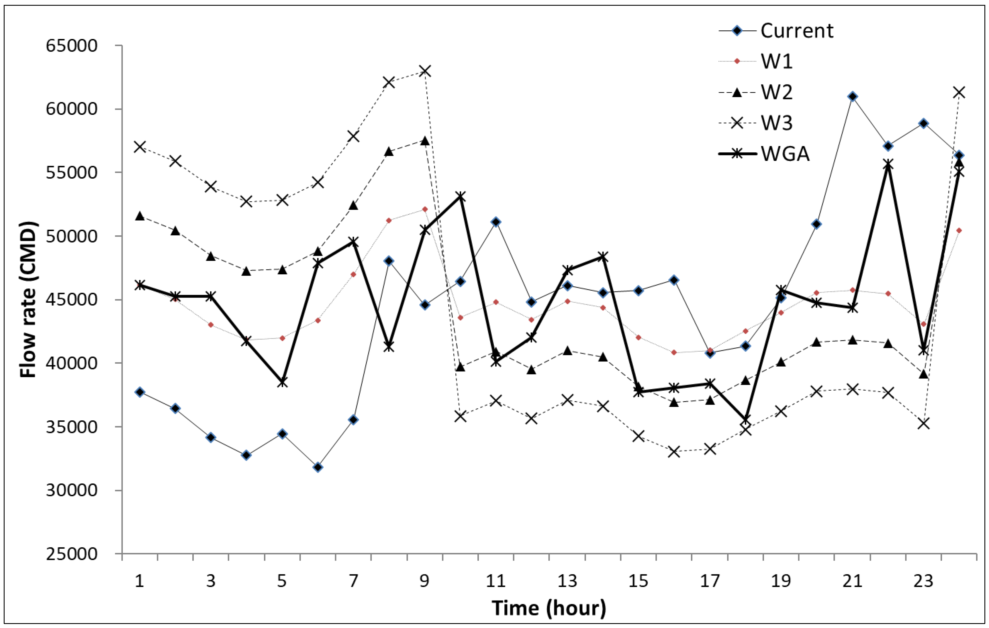
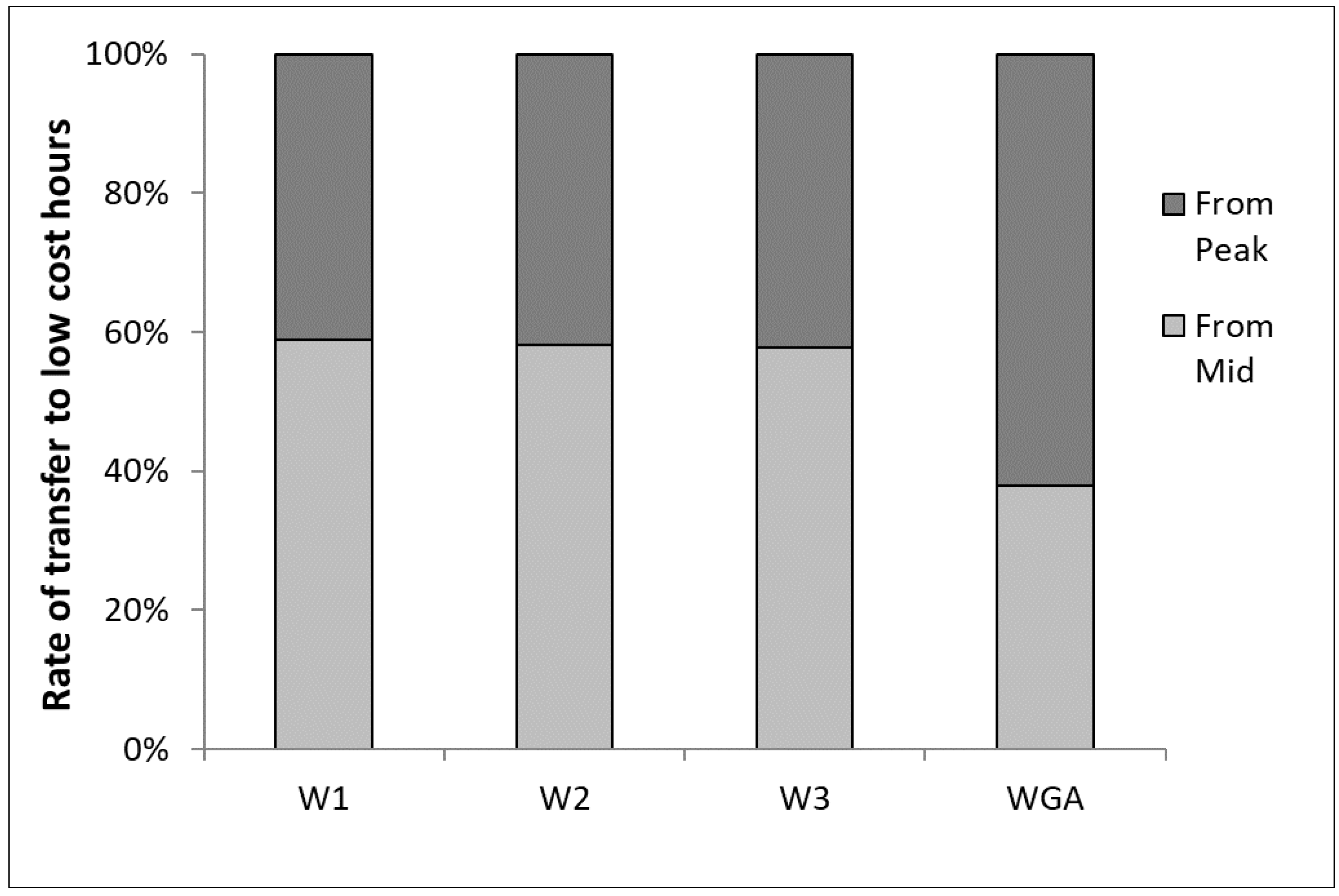
4.3. Winter Season
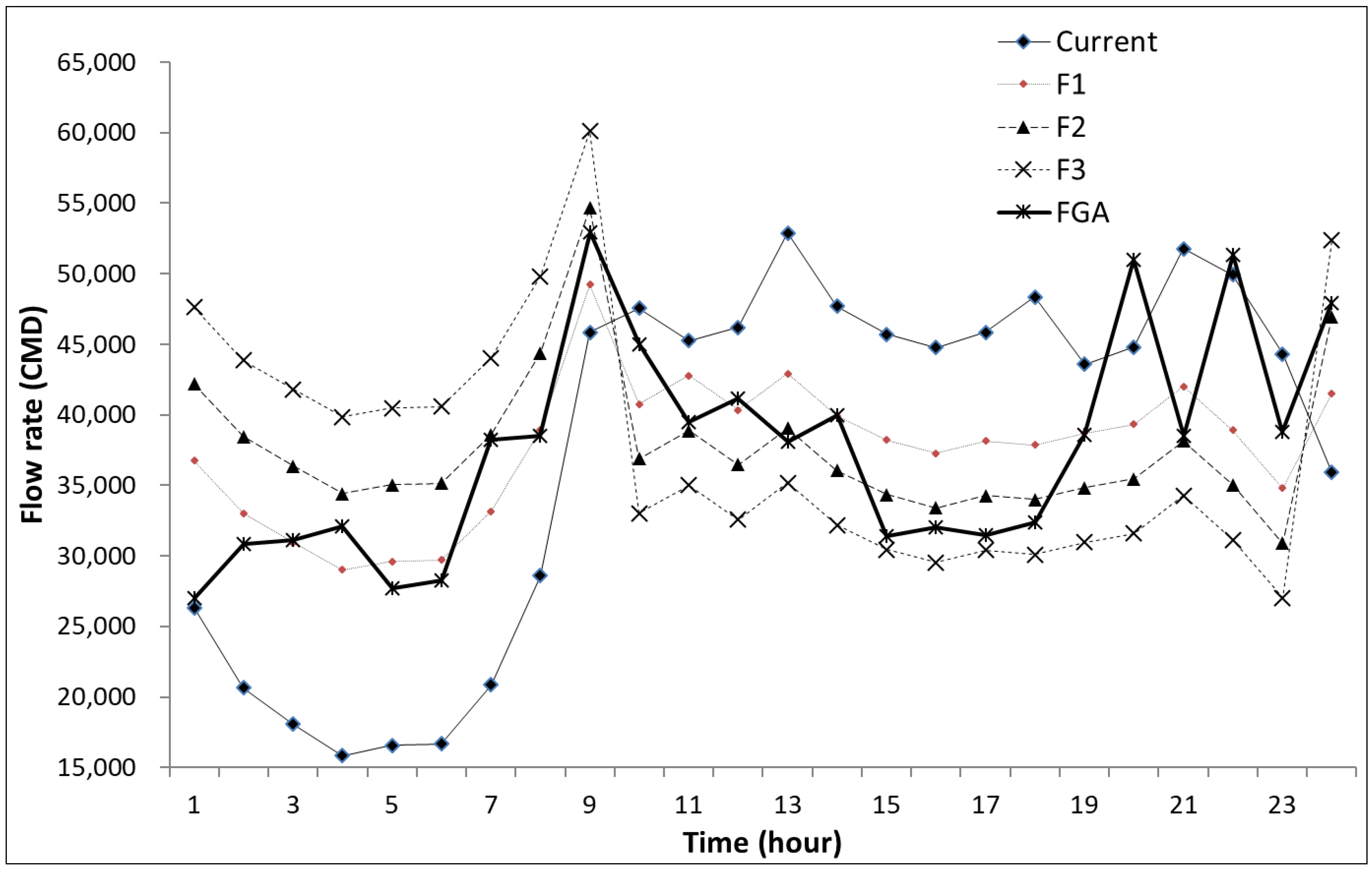
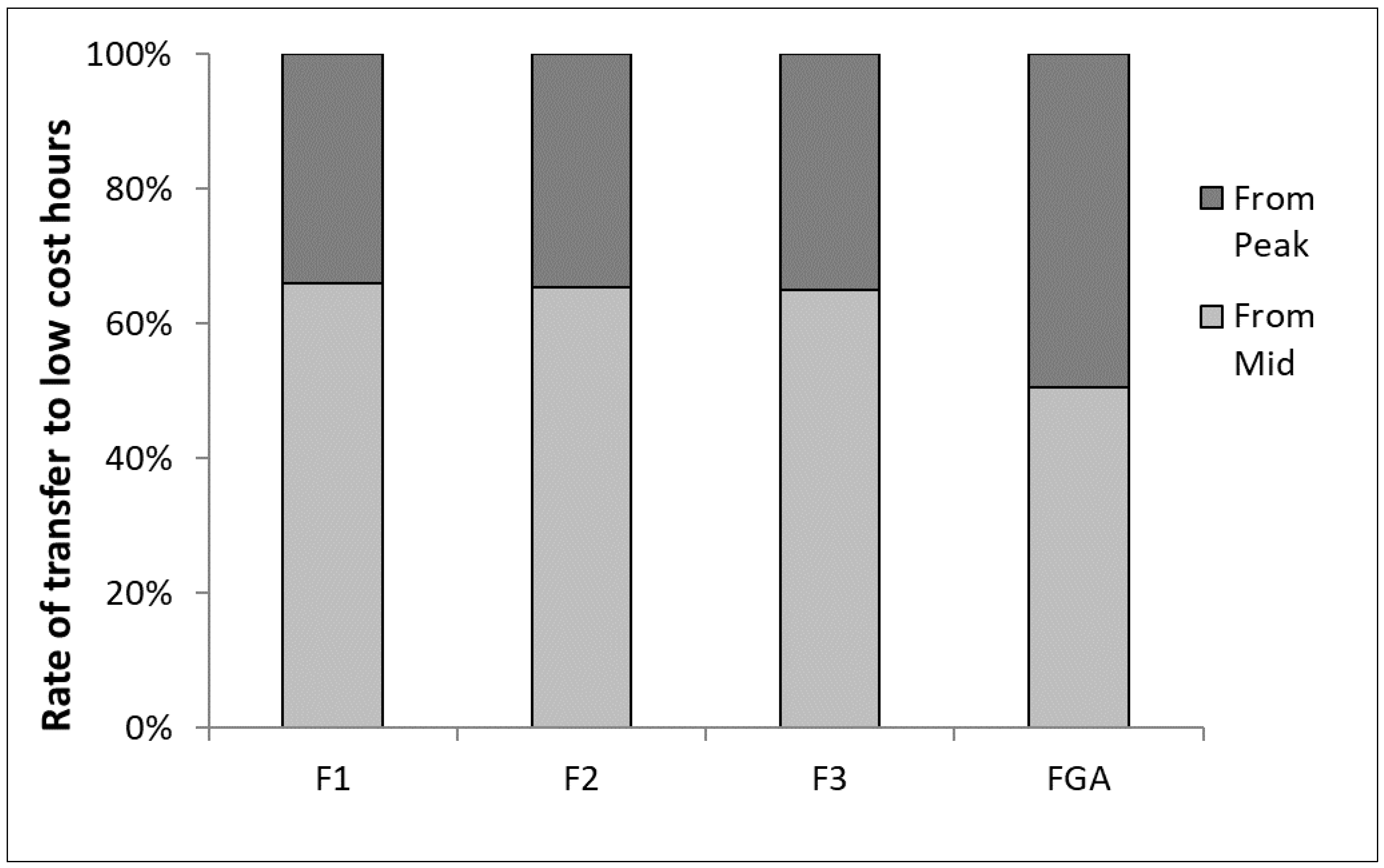
4.4. Spring and Autumn Seasons
4.5. Energy Cost Savings
5. Conclusions
Acknowledgments
Author Contributions
Conflicts of Interest
References
- OECD/IEA. Energy Policies of IEA Countries—The Republic of Korea 2012 Review; International Energy Agency: Paris, France, 2012. [Google Scholar]
- Fan, L.; Wang, F.; Liu, G.; Yang, X.; Qin, W. Public Perception of Water Consumption and Its Effects on Water Conservation Behavior. Water 2014, 6, 1771–1784. [Google Scholar] [CrossRef]
- K-Water. Development of Domestic Estimation Model for Rational Prediction of Water Use (1st Year); K-Water: Daejeon, Korea, 2007. [Google Scholar]
- Byeon, S.; Choi, G.; Maeng, S.; Gourbesville, P. Sustainable Water Distribution Strategy with Smart Water Grid. Sustainability 2015, 7, 4240–4259. [Google Scholar] [CrossRef]
- Woo, D.; Kim, S.; Shin, S.; Kim, J.; Jung, J. Water treatment process settings according to blending alternative resources in Smart Water Grid Research in Korea. In Proceedings of the Smart Water Grid International Conference, Incheon, Korea, 12–14 November 2013. [Google Scholar]
- Gonçalves, F.V.; Ramos, H.M.; Reis, L.F.R. Hybrid energy system evaluation in water supply system energy production: Neural network approach. Int. J. Energy Environ. 2010, 1, 10. [Google Scholar]
- Gorev, N.B.; Kodzhespirova, I.F. Noniterative Implementation of Pressure-Dependent Demands Using the Hydraulic Analysis Engine of EPANET 2. Water Resour. Manag. 2013, 27, 3623–3630. [Google Scholar] [CrossRef]
- Kim, J.; Kim, H.; Lee, D.; Kim, G. Analysis of water use characteristics by household demand monitoring. J. KSEE 2007, 29, 864–869. [Google Scholar]
- Kanakoudis, V.; Tsitsifli, S. Using the bimonthly water balance of a non-fully monitored water distribution network with seasonal water demand peaks to define its actual NRW level: The case of Kos town, Greece. Urban Water J. 2013, 11, 348–360. [Google Scholar] [CrossRef]
- Myoung, S.; Lee, D.; Kim, H.; Jo, J. A comparison of statistical prediction models in household water end-uses. Korean J. Appl. Stat. 2011, 24, 567–573. [Google Scholar] [CrossRef]
- Kim, J.; Lee, D.; Choi, D.; Bae, C.; Park, S. Leakage monitoring model by demand pattern analysis in water distribution systems. In Proceedings of the 2012 Korea Water Resources Association Annual Conference, Taebaek-si, Gangwon, Korea, 17–18 May 2012; pp. 479–483. [Google Scholar]
- Kanakoudis, V.; Gonelas, K. Analysis and calculation of the short and long run economic leakage level in a water distribution system. Water Util. J. 2016, 12, 57–66. [Google Scholar]
- Kanakoudis, V.; Gonelas, K. The joint effect of water price changes and pressure management, at the economic annual real losses level, on the system input volume of a water distribution system. Water Sci. Technol. Water Supply 2015, 15, 1069–1078. [Google Scholar] [CrossRef]
- Seo, J.S.; Lee, D.R.; Choi, S.J.; Kang, S.K. Change of water consumption results from water demand management. In Proceedings of the 2011 Annual Conference of Korea Water Resources Association, Daegu, Korea, 19–20 May 2011. [Google Scholar]
- Hwang, J.W.; Lee, H.D.; Choi, J.H.; Bae, C.H. Assessment of hydraulic behavior and water quality variation characteristics in underground reservoir of building. In Proceedings of the 2005 Annual Conference of Korean Society of Water and Wastewater, Gwangju, Korea, 10–11 November 2005; pp. 401–404. [Google Scholar]
- Kwak, P.J.; Hwang, J.W.; Kim, S.K.; Lee, H.D. Hydraulic behavior and water quality variation characteristics in underground reservoir. In Proceedings of the 2005 Annual Conference of Korean Society of Civil Engineers, Jeju, Korea, 20–21 October 2005; pp. 364–367. [Google Scholar]
- Kanakoudis, V.; Tolikas, D. The Role of Leaks and Breaks in Water Networks—Technical and Economical Solutions. J. Water Supply Res. Technol. 2001, 50, 301–311. [Google Scholar]
- Kanakoudis, V.; Tolikas, D. Assessing the Performance Level of a Water System. Water Air Soil Pollut. Focus 2004, 4, 307–318. [Google Scholar] [CrossRef]
- Kanakoudis, V.; Tsitsifli, S. Potable water security assessment—A review on monitoring, modelling and optimization techniques, applied to water distribution networks. Desalin. Water Treat. 2017, 99, 18–26. [Google Scholar] [CrossRef]
- Kanakoudis, V.; Gonelas, K. Developing a Methodology towards Full Water Cost Recovery in Urban Water Pipe Networks, based on the “User-pays” Principle. Procedia Eng. 2014, 70, 907–916. [Google Scholar] [CrossRef]
- Kanakoudis, V.; Gonelas, K.; Tolikas, D. Basic principles for urban water value assessment and price setting towards its full cost recovery—Pinpointing the role of the water losses. J. Water Supply Res. Technol. 2011, 60, 27–39. [Google Scholar] [CrossRef]
- Moon, S.I. The smart grid, future of electricity. Sci. Technol. 2009, 42, 56–59. [Google Scholar]
- Kanakoudis, V. Vulnerability based management of water resources systems. J. Hydroinform. 2004, 6, 133–156. [Google Scholar]
- Jeon, S. Problem and Measures to Improve Pricing System of Electricity; Korean National Assembly Budget Office: Seoul, Korea, 2013. [Google Scholar]
- Patelis, M.; Kanakoudis, V.; Gonelas, K. Combining pressure management and energy recovery benefits in a water distribution system installing PATs. J. Water Supply Res. Technol. 2017, 66, 520–527. [Google Scholar] [CrossRef]
- Eusuff, M.M.; Lansey, K.E. Optimization of water distribution network design using the shuffled frog leaping algorithm. J. Water Resour. Plan. Manag. 2003, 129, 210–225. [Google Scholar] [CrossRef]
- Patelis, M.; Kanakoudis, V.; Gonelas, K. Pressure management and energy recovery capabilities using PATs. Procedia Eng. 2016, 162, 503–510. [Google Scholar] [CrossRef]
- Savic, D.A.; Walters, G.A. Genetic Algorithms for the least-cost design of water distribution networks. J. Water Resour. Plan. Manag. 1997, 123, 67–77. [Google Scholar] [CrossRef]
- Rossman, L.A. Epanet 2 Users Manual; EPA/600/R-00/057; U.S. Environmental Protection Agency: Washington, DC, USA, 2000.
- Eliades, D.G.; Kyriakou, M.; Vrachimis, S.; Polycarpou, M.M. EPANET-MATLAB toolkit: An open-source software for interfacing EPANET with MATLAB. Zenodo 2017. [Google Scholar] [CrossRef]
- Korkana, P.; Kanakoudis, V.; Makrysopoulos, A.; Patelis, M.; Gonelas, K. Developing an optimization algorithm to form district metered areas in a water distribution system. Procedia Eng. 2016, 162, 530–536. [Google Scholar] [CrossRef][Green Version]
- Korkana, P.; Kanakoudis, V.; Patelis, M.; Gonelas, K. Forming District Metered Areas in a Water Distribution Network Using Genetic Algorithms. Procedia Eng. 2016, 162, 511–520. [Google Scholar] [CrossRef]
- Chondronasios, A.; Gonelas, K.; Kanakoudis, V.; Patelis, M.; Korkana, P. Optimizing DMAs’ formation in a water pipe network: The water aging and the operating pressure factors. J. Hydroinform. 2017, 19, 890–899. [Google Scholar] [CrossRef]
- Prasad, M.; Bajpai, R.; Shashidhara, L.S. Regulation of wingless and vestigial expression in wing and haltere discs of drosophila. Development 2003, 130, 1537–1547. [Google Scholar] [CrossRef] [PubMed]
- Prasad, T.D.; Park, N.S. Objective Genetic Algorithms for design of water distribution networks. J. Water Resour. Plan. Manag. 2004, 130, 73–82. [Google Scholar] [CrossRef]
- Deb, K.; Jain, H. An evolutionary many-objective optimization algorithm using reference-point-based nondominated sorting approach, part I: Solving problems with box constraints. IEEE Trans. Evolut. Comput. 2014, 18, 577–601. [Google Scholar] [CrossRef]
- Gutierrez-Antonio, C.; Briones-Ramirez, A. Pareto front of ideal petlyuk sequences using a multiobjective genetic algorithm with constraints. Comput. Chem. Eng. 2009, 33, 454–464. [Google Scholar] [CrossRef]
- Coello, A.C. Theoretical and Numerical Constraint-Handling Techniques Used with Evolutionary Algorithms: A Survey of the State of the Art. Comput. Methods Appl. Mech. Eng. 2002, 191, 1245–1287. [Google Scholar] [CrossRef]
- Jakob, W.; Blume, C. Pareto Optimization or Cascaded Weighted Sum: A Comparison of Concepts. Algorithms 2014, 7, 166–185. [Google Scholar] [CrossRef]


| Year | Cost Level | Unit Price US Dollar/kW h | Intake St. (%) | Pumping St. (%) | Water distribution Networks (WDNs) (%) |
|---|---|---|---|---|---|
| 2011 | High | 0.193 | 47.9 | 47.9 | 46.2 |
| Middle | 0.112 | 35.5 | 35.5 | 36.8 | |
| Low | 0.059 | 16.6 | 16.6 | 17.0 | |
| 2012 | High | 0.193 | 47.0 | 47.2 | 45.1 |
| Middle | 0.112 | 35.5 | 35.4 | 36.7 | |
| Low | 0.059 | 17.5 | 17.4 | 18.2 |
| Building Type and Minimum Criteria of Water Storage Facility Necessity | No. of Storage Facilities |
|---|---|
| General buildings larger than 5000 m2 | 816 |
| Commercial buildings larger than 3000 m2 | 334 |
| Complex buildings lager than 2000 m2 | 450 |
| Theaters | 2 |
| Private academies over 2000 m2 | 2 |
| Large shops at individual buildings | 6 |
| Wedding halls over 2000 m2 | 12 |
| Indoor gyms | 4 |
| Apartment complexes | 1067 |
| Total | 2693 |
| Storage Capacity (m3) | No. of Facilities | Sum of Daily Mean Water Demand (m3/day) |
|---|---|---|
| 1–10 | 18 | 106 |
| 11–50 | 70 | 1718 |
| 51–100 | 14 | 890 |
| 101–500 | 13 | 2976 |
| 501–1000 | 7 | 5631 |
| Total | 122 | 11,321 |
| Procedure | Parameter Name | Value | Remarks |
|---|---|---|---|
| Real number coding | Length of chromosome | L = 24 | |
| Population | Population | 50 | |
| Linear ranking | Crowding degree of crossover | ||
| Crossover | Crossover ratio | 0–50% | Randomly varying in generations |
| Mutation | Maximum generation | 0–10% | Randomly varying in generations |
| Scaling window | Scaling window | ||
| Elitist selection | Survived generation | 1 |
| Season | Case Name | Description |
|---|---|---|
| Summer | SP | Current State |
| S1 | Uniform distribution of 60% demand of storage facility at low price hours | |
| S2 | Uniform distribution of 80% demand of storage facility at low price hours | |
| S3 | Uniform distribution of 100% demand of storage facility at low price hours | |
| SGA | Distribution optimization by genetic algorithm | |
| Winter | WP | Current State |
| W1 | Uniform distribution of 60% demand of storage facility at low price hours | |
| W2 | Uniform distribution of 80% demand of storage facility at low price hours | |
| W3 | Uniform distribution of 100% demand of storage facility at low price hours | |
| WGA | Distribution optimization by genetic algorithm | |
| Spring and Autumn | FP | Current State |
| F1 | Uniform distribution of 60% demand of storage facility at low price hours | |
| F2 | Uniform distribution of 80% demand of storage facility at low price hours | |
| F3 | Uniform distribution of 100% demand of storage facility at low price hours | |
| FGA | Distribution optimization by genetic algorithm |
| Time | Cost Level | Hourly Flow Rate (m3/h) | Difference with Current (m3) | |||||||
|---|---|---|---|---|---|---|---|---|---|---|
| Current | S1 | S2 | S3 | SGA | S1 | S2 | S3 | SGA | ||
| 1 | Low | 1563 | 1593 | 1819 | 2046 | 1363 | −30 | −257 | −483 | 200 |
| 2 | 1422 | 1436 | 1662 | 1889 | 1409 | −13 | −240 | −466 | 13 | |
| 3 | 1355 | 1358 | 1584 | 1810 | 1232 | −3 | −229 | −456 | 123 | |
| 4 | 996 | 1164 | 1390 | 1617 | 1151 | −168 | −394 | −621 | −155 | |
| 5 | 777 | 1179 | 1405 | 1631 | 1237 | −401 | −628 | −854 | −460 | |
| 6 | 767 | 1197 | 1423 | 1649 | 895 | −430 | −656 | −883 | −128 | |
| 7 | 905 | 1305 | 1531 | 1758 | 1542 | −400 | −626 | −853 | −637 | |
| 8 | 1120 | 1491 | 1718 | 1944 | 1674 | −371 | −598 | −824 | −554 | |
| 9 | 1441 | 1738 | 1964 | 2191 | 1918 | −297 | −523 | −749 | −477 | |
| 10 | Mid | 1761 | 1497 | 1335 | 1173 | 1552 | 264 | 426 | 587 | 209 |
| 11 | 1854 | 1538 | 1376 | 1215 | 1577 | 316 | 478 | 640 | 278 | |
| 12 | Peak | 1794 | 1574 | 1412 | 1251 | 1255 | 220 | 382 | 543 | 539 |
| 13 | Mid | 1799 | 1568 | 1406 | 1244 | 1465 | 232 | 394 | 555 | 334 |
| 14 | Peak | 1634 | 1598 | 1436 | 1274 | 1397 | 37 | 198 | 360 | 238 |
| 15 | 1535 | 1493 | 1331 | 1169 | 1338 | 42 | 204 | 365 | 197 | |
| 16 | 1567 | 1451 | 1289 | 1127 | 1247 | 117 | 278 | 440 | 320 | |
| 17 | 1584 | 1403 | 1241 | 1080 | 1169 | 181 | 342 | 504 | 415 | |
| 18 | Mid | 1500 | 1402 | 1241 | 1079 | 1206 | 97 | 259 | 421 | 294 |
| 19 | 1402 | 1434 | 1272 | 1110 | 1516 | −32 | 130 | 292 | −114 | |
| 20 | 1552 | 1481 | 1320 | 1158 | 1853 | 71 | 232 | 394 | −301 | |
| 21 | 1575 | 1472 | 1310 | 1148 | 1626 | 103 | 265 | 427 | −51 | |
| 22 | 1667 | 1387 | 1225 | 1063 | 1767 | 281 | 442 | 604 | −99 | |
| 23 | 1641 | 1359 | 1197 | 1036 | 1500 | 282 | 444 | 606 | 141 | |
| 24 | Low | 1460 | 1556 | 1782 | 2009 | 1784 | −96 | −322 | −549 | −324 |
| Summary | Low | 11,806 | 14,015 | 16,279 | 18,544 | 14,265 | −2209 | −4474 | −6738 | −2459 |
| Mid | 14,752 | 13,138 | 11,682 | 10,227 | 13,751 | 1614 | 3070 | 4525 | 1000 | |
| Peak | 8114 | 7518 | 6709 | 5901 | 6655 | 596 | 1404 | 2213 | 1459 | |
| Time | Cost Level | Hourly Flow Rate (m3/h) | Difference with Current (m3) | |||||||
|---|---|---|---|---|---|---|---|---|---|---|
| Current | W1 | W2 | W3 | WGA | W1 | W2 | W3 | WGA | ||
| 1 | Low | 1573 | 1924 | 2150 | 2376 | 1923 | −351 | −577 | −804 | −351 |
| 2 | 1518 | 1876 | 2102 | 2329 | 1885 | −357 | −584 | −810 | −366 | |
| 3 | 1422 | 1793 | 2019 | 2246 | 1886 | −371 | −597 | −823 | −464 | |
| 4 | 1364 | 1744 | 1970 | 2197 | 1740 | −380 | −606 | −833 | −376 | |
| 5 | 1436 | 1749 | 1975 | 2202 | 1605 | −313 | −539 | −766 | −169 | |
| 6 | 1326 | 1807 | 2033 | 2260 | 1994 | −481 | −708 | −934 | −668 | |
| 7 | 1482 | 1958 | 2185 | 2411 | 2064 | −477 | −703 | −929 | −582 | |
| 8 | 2002 | 2135 | 2362 | 2588 | 1721 | −133 | −360 | −586 | 281 | |
| 9 | 1858 | 2171 | 2398 | 2624 | 2105 | −314 | −540 | −766 | −248 | |
| 10 | Mid | 1935 | 1817 | 1655 | 1493 | 2213 | 118 | 280 | 441 | −278 |
| 11 | 2130 | 1867 | 1705 | 1544 | 1671 | 263 | 425 | 587 | 459 | |
| 12 | Peak | 1868 | 1809 | 1647 | 1486 | 1751 | 59 | 220 | 382 | 117 |
| 13 | Mid | 1921 | 1870 | 1708 | 1547 | 1971 | 51 | 213 | 374 | −50 |
| 14 | Peak | 1898 | 1849 | 1687 | 1526 | 2016 | 49 | 210 | 372 | −118 |
| 15 | 1904 | 1751 | 1590 | 1428 | 1572 | 153 | 315 | 477 | 333 | |
| 16 | 1940 | 1701 | 1539 | 1378 | 1585 | 239 | 401 | 563 | 355 | |
| 17 | 1700 | 1709 | 1547 | 1386 | 1599 | −9 | 153 | 314 | 101 | |
| 18 | Mid | 1722 | 1773 | 1611 | 1449 | 1482 | −50 | 112 | 273 | 241 |
| 19 | 1880 | 1833 | 1672 | 1510 | 1907 | 47 | 209 | 371 | −26 | |
| 20 | 2122 | 1898 | 1737 | 1575 | 1866 | 224 | 385 | 547 | 256 | |
| 21 | 2541 | 1906 | 1744 | 1582 | 1849 | 635 | 797 | 958 | 692 | |
| 22 | 2379 | 1894 | 1733 | 1571 | 2,321 | 484 | 646 | 808 | 58 | |
| 23 | 2454 | 1794 | 1632 | 1471 | 1,710 | 660 | 821 | 983 | 744 | |
| 24 | Low | 2349 | 2102 | 2328 | 2554 | 2,295 | 248 | 21 | −205 | 54 |
| Summary | Low | 16,330 | 19,258 | 21,523 | 23,787 | 19,218 | −2928 | −5193 | −7457 | −2888 |
| Mid | 16,217 | 14,498 | 13,204 | 11,910 | 15,126 | 1720 | 3014 | 4308 | 1091 | |
| Peak | 12,177 | 10,974 | 10,004 | 9034 | 10,386 | 1202 | 2173 | 3143 | 1791 | |
| Time | Cost Level | Hourly Flow Rate (m3/h) | Difference with Current (m3) | |||||||
|---|---|---|---|---|---|---|---|---|---|---|
| Current | F1 | F2 | F3 | FGA | F1 | F2 | F3 | FGA | ||
| 1 | Low | 1097 | 1532 | 1758 | 1985 | 1125 | −435 | −662 | −888 | −28 |
| 2 | 861 | 1375 | 1602 | 1828 | 1284 | −514 | −741 | −967 | −423 | |
| 3 | 752 | 1288 | 1515 | 1741 | 1298 | −536 | −762 | −989 | −545 | |
| 4 | 660 | 1208 | 1435 | 1661 | 1336 | −548 | −775 | −1001 | −676 | |
| 5 | 690 | 1234 | 1460 | 1686 | 1156 | −544 | −770 | −996 | −466 | |
| 6 | 694 | 1238 | 1464 | 1691 | 1179 | −544 | −770 | −997 | −485 | |
| 7 | 869 | 1382 | 1609 | 1,835 | 1594 | −513 | −739 | −966 | −725 | |
| 8 | 1191 | 1623 | 1850 | 2076 | 1605 | −432 | −658 | −885 | −414 | |
| 9 | 1911 | 2052 | 2278 | 2504 | 2206 | −141 | −367 | −594 | −296 | |
| 10 | Mid | 1982 | 1699 | 1537 | 1375 | 1875 | 283 | 445 | 606 | 107 |
| 11 | 1885 | 1782 | 1620 | 1459 | 1644 | 103 | 265 | 426 | 241 | |
| 12 | Peak | 1925 | 1681 | 1519 | 1357 | 1714 | 244 | 406 | 567 | 210 |
| 13 | Mid | 2204 | 1789 | 1627 | 1465 | 1588 | 415 | 577 | 738 | 616 |
| 14 | Peak | 1987 | 1664 | 1502 | 1341 | 1667 | 323 | 484 | 646 | 320 |
| 15 | 1904 | 1592 | 1430 | 1269 | 1309 | 312 | 474 | 635 | 595 | |
| 16 | 1865 | 1554 | 1392 | 1230 | 1334 | 311 | 473 | 635 | 531 | |
| 17 | 1910 | 1590 | 1428 | 1266 | 1312 | 320 | 482 | 644 | 598 | |
| 18 | Mid | 2014 | 1578 | 1416 | 1254 | 1348 | 437 | 598 | 760 | 667 |
| 19 | 1816 | 1613 | 1451 | 1290 | 1608 | 204 | 365 | 527 | 209 | |
| 20 | 1866 | 1639 | 1478 | 1316 | 2126 | 227 | 389 | 551 | −259 | |
| 21 | 2157 | 1751 | 1589 | 1428 | 1605 | 406 | 568 | 729 | 552 | |
| 22 | 2080 | 1621 | 1459 | 1298 | 2139 | 458 | 620 | 782 | −60 | |
| 23 | 1846 | 1449 | 1288 | 1126 | 1617 | 397 | 558 | 720 | 228 | |
| 24 | Low | 1497 | 1731 | 1957 | 2184 | 1996 | −234 | −461 | −687 | −499 |
| Summary | Low | 10,222 | 14,663 | 16,927 | 19,191 | 14,780 | −4441 | −6705 | −8969 | −4558 |
| Mid | 17,851 | 14,921 | 13,466 | 12,010 | 15,550 | 2929 | 4385 | 5840 | 2301 | |
| Peak | 9591 | 8081 | 7272 | 6463 | 7336 | 1510 | 2319 | 3127 | 2255 | |
| Hour | Summer Season | Winter Season | Spring–Autumn | |||||||||
|---|---|---|---|---|---|---|---|---|---|---|---|---|
| Cost (USD) | Base | S1 | SGA | Cost (USD) | Base | W1 | WGA | Cost (USD) | Base | F1 | FGA | |
| 1 | 0.059 | 92 | 94 | 82 | 0.065 | 103 | 126 | 126 | 0.065 | 65 | 91 | 66 |
| 2 | 0.059 | 84 | 85 | 82 | 0.065 | 99 | 122 | 123 | 0.065 | 51 | 81 | 76 |
| 3 | 0.059 | 80 | 80 | 77 | 0.065 | 93 | 117 | 123 | 0.065 | 44 | 76 | 77 |
| 4 | 0.059 | 59 | 69 | 78 | 0.065 | 89 | 114 | 114 | 0.065 | 39 | 71 | 79 |
| 5 | 0.059 | 46 | 70 | 61 | 0.065 | 94 | 114 | 105 | 0.065 | 41 | 73 | 68 |
| 6 | 0.059 | 45 | 71 | 73 | 0.065 | 87 | 118 | 130 | 0.065 | 41 | 73 | 70 |
| 7 | 0.059 | 53 | 77 | 92 | 0.065 | 97 | 128 | 135 | 0.065 | 51 | 82 | 94 |
| 8 | 0.059 | 66 | 88 | 82 | 0.065 | 131 | 139 | 112 | 0.065 | 70 | 96 | 95 |
| 9 | 0.059 | 85 | 103 | 112 | 0.065 | 121 | 142 | 137 | 0.065 | 113 | 121 | 130 |
| 10 | 0.112 | 198 | 168 | 216 | 0.110 | 214 | 201 | 244 | 0.110 | 163 | 140 | 155 |
| 11 | 0.112 | 208 | 173 | 154 | 0.166 | 353 | 309 | 277 | 0.166 | 155 | 147 | 135 |
| 12 | 0.193 | 345 | 303 | 296 | 0.166 | 309 | 300 | 290 | 0.166 | 216 | 189 | 193 |
| 13 | 0.112 | 202 | 176 | 155 | 0.110 | 212 | 206 | 218 | 0.110 | 182 | 147 | 131 |
| 14 | 0.193 | 315 | 308 | 310 | 0.110 | 210 | 204 | 223 | 0.110 | 223 | 187 | 187 |
| 15 | 0.193 | 295 | 287 | 232 | 0.110 | 210 | 193 | 174 | 0.110 | 214 | 179 | 147 |
| 16 | 0.193 | 302 | 279 | 226 | 0.110 | 214 | 188 | 175 | 0.110 | 210 | 175 | 150 |
| 17 | 0.193 | 305 | 270 | 216 | 0.110 | 188 | 189 | 177 | 0.110 | 215 | 179 | 147 |
| 18 | 0.112 | 168 | 157 | 130 | 0.166 | 285 | 294 | 245 | 0.166 | 166 | 130 | 111 |
| 19 | 0.112 | 157 | 161 | 158 | 0.166 | 311 | 304 | 316 | 0.166 | 150 | 133 | 132 |
| 20 | 0.112 | 174 | 166 | 190 | 0.166 | 351 | 314 | 309 | 0.166 | 154 | 135 | 175 |
| 21 | 0.112 | 177 | 165 | 149 | 0.110 | 280 | 210 | 204 | 0.110 | 178 | 144 | 132 |
| 22 | 0.112 | 187 | 156 | 199 | 0.110 | 263 | 209 | 256 | 0.110 | 171 | 134 | 176 |
| 23 | 0.112 | 184 | 152 | 192 | 0.166 | 406 | 297 | 283 | 0.166 | 152 | 119 | 133 |
| 24 | 0.059 | 86 | 92 | 103 | 0.065 | 153 | 137 | 150 | 0.065 | 88 | 102 | 118 |
| Sum | 3915 | 3750 | 3667 | 4873 | 4675 | 4645 | 3153 | 3004 | 2979 | |||
| Reduce Rate (%) | 4.22 | 6.33 | 4.06 | 4.69 | 4.71 | 5.51 | ||||||
| Month | Pumping Energy Cost (US Dollar) | Reduction Rate | Estimated Reduction (US Dollar) | ||||
|---|---|---|---|---|---|---|---|
| Water treatment plant (WTP) to Reservoir | Intake to WTP | Intake Pump | WTP to Reservoir | Intake to WTP | Intake Pump | ||
| 1 | 217,187 | 374,619 | 198,833 | 4.69 | 10,186 | 17,570 | 9325 |
| 2 | 204,927 | 368,949 | 195,837 | 4.69 | 9611 | 17,304 | 9185 |
| 3 | 163,857 | 295,386 | 159,691 | 5.51 | 9029 | 16,276 | 8799 |
| 4 | 158,186 | 284,807 | 152,206 | 5.51 | 8716 | 15,693 | 8387 |
| 5 | 161,967 | 265,562 | 143,691 | 5.51 | 8924 | 14,632 | 7917 |
| 6 | 162,426 | 277,781 | 150,808 | 5.51 | 8950 | 15,306 | 8310 |
| 7 | 208,737 | 363,752 | 194,557 | 6.33 | 13,213 | 23,026 | 12,315 |
| 8 | 231,201 | 392,057 | 209,807 | 6.33 | 14,635 | 24,817 | 13,281 |
| 9 | 178,433 | 288,754 | 157,592 | 5.51 | 9832 | 15,910 | 8683 |
| 10 | 187,814 | 314,747 | 177,283 | 5.51 | 10,349 | 17,343 | 9768 |
| 11 | 220,807 | 359,276 | 201,406 | 4.69 | 10,356 | 16,850 | 9446 |
| 12 | 224,347 | 343,844 | 189,648 | 4.69 | 10,522 | 16,126 | 8894 |
| Total | 2,319,890 | 3,929,535 | 2,131,360 | - | 124,322 | 210,852 | 114,311 |
© 2018 by the authors. Licensee MDPI, Basel, Switzerland. This article is an open access article distributed under the terms and conditions of the Creative Commons Attribution (CC BY) license (http://creativecommons.org/licenses/by/4.0/).
Share and Cite
Chang, Y.; Choi, G.; Kim, J.; Byeon, S. Energy Cost Optimization for Water Distribution Networks Using Demand Pattern and Storage Facilities. Sustainability 2018, 10, 1118. https://doi.org/10.3390/su10041118
Chang Y, Choi G, Kim J, Byeon S. Energy Cost Optimization for Water Distribution Networks Using Demand Pattern and Storage Facilities. Sustainability. 2018; 10(4):1118. https://doi.org/10.3390/su10041118
Chicago/Turabian StyleChang, Yungyu, Gyewoon Choi, Juhwan Kim, and Seongjoon Byeon. 2018. "Energy Cost Optimization for Water Distribution Networks Using Demand Pattern and Storage Facilities" Sustainability 10, no. 4: 1118. https://doi.org/10.3390/su10041118
APA StyleChang, Y., Choi, G., Kim, J., & Byeon, S. (2018). Energy Cost Optimization for Water Distribution Networks Using Demand Pattern and Storage Facilities. Sustainability, 10(4), 1118. https://doi.org/10.3390/su10041118