New Integrated Quality Function Deployment Approach Based on Interval Neutrosophic Set for Green Supplier Evaluation and Selection


Abstract
:
1. Introduction
2. Preliminary
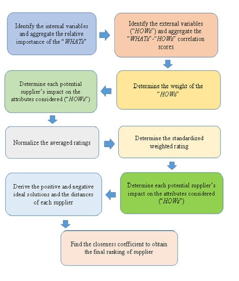
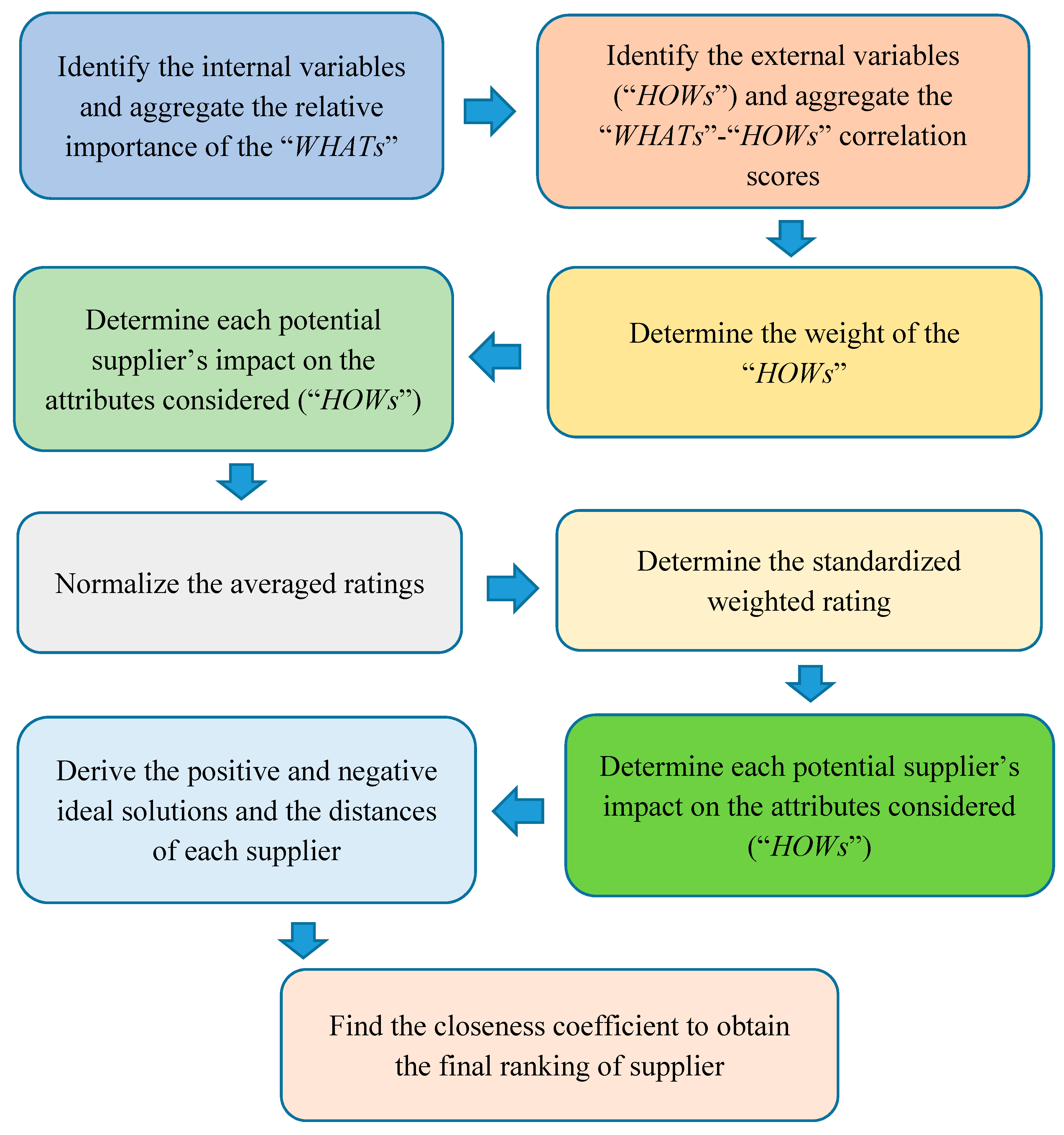
3. QFD Model Development Using Interval Neutrosophic Sets
3.1. Identify the Characteristics That the Product Being Purchased Must Have (Internal Variables or “WHATs”) to Meet the Company’s Needs and Aggregate the Relative Importance of “WHATs”
3.2. Identify the Criteria Relevant to Supplier Assessment (External Variables or “HOWs”) and Aggregate the “WHATs”-“HOWs” Correlation Scores
3.3. Determine the Weights of the “HOWs” Criteria
3.4. Determine Each Potential Supplier Impact on the Attributes Considered “HOWs”
3.5. Normalize the Averaged Ratings
3.6. Determine the Standardized Weighted Rating
3.7. Derive and
3.8. Find the Closeness Coefficient and Ranking Order of Alternatives
4. Application of the Proposed Model for Green Supplier Evaluation and Selection
4.1. Aggregate the Importance Weights of the “WHATs”
4.2. Aggregate the “HOWs”-“WHATs” Correlation Scores
4.3. Aggregate the Importance Weights of the “HOWs”
4.4. Determine Each Potential Supplier’s Impacts on the Attributes Considered the “HOWs”
4.5. Normalize the Averaged Ratings and Weights of the “HOWs”
4.6. Determine the Standardized Weighted Rating
4.7. Derive and
4.8. Find the Closeness Coefficient and Ranking Order of Each Supplier
5. Discussion and Conclusions
Acknowledgement
Author Contributions
Conflicts of Interest
References
- Yazdani, M.; Hashemkhani Zolfani, S.; Zavadskas, E.K. New integration of MCDM methods and QFD in the selection of green suppliers. J. Bus. Econ. Manag. 2016, 17, 1097–1113. [Google Scholar] [CrossRef]
- Tavana, M.; Yazdani, M.; Caprio, D.D. An application of an integrated ANP-QFD framework for sustainable supplier selection. Int. J. Logist. Res. Appl. 2017, 20, 254–275. [Google Scholar] [CrossRef]
- Hashemkhani Zolfani, S.; Maknoon, R.; Zavadskas, E.K. An introduction to prospective multiple attribute decision making (PMADM). Technol. Econ. Dev. Econ. 2016, 22, 309–326. [Google Scholar] [CrossRef]
- Hashemkhani Zolfani, S.; Maknoon, R.; Zavadskas, E.K. Multiple attribute decision making (MADM) based scenarios. Int. J. Strateg. Prop. Manag. 2016, 20, 101–111. [Google Scholar] [CrossRef]
- Kumar, A.; Jain, V.; Kumar, S. A comprehensive environment friendly approach for supplier selection. Omega 2014, 42, 109–123. [Google Scholar] [CrossRef]
- Grisi, R.M.; Guerra, L.; Naviglio, G. Supplier performance evaluation for green supply chainmanagement. In Business Performance Measurement and Management; Springer: Berlin/Heidelberg, Germany, 2010; Chapter 10; pp. 149–163. [Google Scholar]
- Abdollahi, M.; Arvan, M.; Razmi, J. An integrated approach for supplier portfolio selection: Lean or agile. Exp. Syst. Appl. 2015, 42, 679–690. [Google Scholar] [CrossRef]
- Hashemi, S.H.; Karimi, A.; Tavana, M. An integrated green supplier selection approach with analytic network process and improved Grey relational analysis. Int. J. Prod. Econ. 2015, 159, 178–191. [Google Scholar] [CrossRef]
- Heidarzade, A.; Mahdavi, I.; Mahdavi-Amiri, N. Supplier selection using a clustering method based on a new distance for interval Type-2 fuzzy sets: A case study. Appl. Soft Comput. 2016, 38, 213–231. [Google Scholar] [CrossRef]
- Junior, F.R.L.; Carpinetti, L.C.R. A multicriteria approach based on fuzzy QFD for choosing criteria for supplier selection. Comput. Ind. Eng. 2016, 101, 269–285. [Google Scholar] [CrossRef]
- Wang, K.-Q.; Liu, H.-C.; Liu, L.; Huang, J. Green supplier evaluation and selection using cloud model theory and the QUALIFLEX method. Sustainability 2017, 9, 688. [Google Scholar] [CrossRef]
- Mafakheri, F.; Breton, M.; Ghoniem, A. Supplier selection order allocation: A two-stage multiple criteria dynamic programming approach. Int. J. Prod. Econ. 2011, 132, 52–57. [Google Scholar] [CrossRef]
- Büyüközkan, G.; Çifçi, G. Evaluation of the green supply chain management practices: A fuzzy ANP approach. Prod. Plan. Control 2012, 23, 405–418. [Google Scholar] [CrossRef]
- Kuo, R.J.; Wang, Y.C.; Tien, F.C. Integration of artificial neural network and MADA methods for green supplier selection. J. Clean. Prod. 2010, 18, 1161–1170. [Google Scholar] [CrossRef]
- Memon, M.S.; Lee, Y.H.; Mari, S.I. Group multi-criteria supplier selection using combined grey systems theory and uncertainty theory. Exp. Syst. Appl. 2015, 42, 7951–7959. [Google Scholar] [CrossRef]
- Wang, W.P. A fuzzy linguistic computing approach to supplier evaluation. Appl. Math. Model. 2010, 34, 3130–3141. [Google Scholar] [CrossRef]
- Chen, Y.J. Structured methodology for supplier selection and evaluation in a supply chain. Inf. Sci. 2011, 181, 1651–1670. [Google Scholar] [CrossRef]
- Zhu, Q.; Dou, Y.; Sarkis, J. A portfolio-based analysis for green supplier management using the analytical network process. Supply Chain Manag. Int. J. 2010, 15, 306–319. [Google Scholar] [CrossRef]
- Tseng, M.L.; Chiu, A.F.S. Evaluating firm’s green supply chain management in linguistic preferences. J. Clean. Prod. 2013, 4, 22–31. [Google Scholar] [CrossRef]
- Punniyamoorthy, M.; Mathiyalagan, P.; Parthiban, P. A strategic model using structural equation modeling and fuzzy logic in supplier selection. Exp. Syst. Appl. 2011, 38, 458–474. [Google Scholar] [CrossRef]
- Shen, C.Y.; Yu, K.T. Enhancing the efficacy of supplier selection decision-making on the initial stage of new product development: A hybrid fuzzy approach considering the strategic and operational factors simultaneously. Exp. Syst. Appl. 2009, 36, 11271–11281. [Google Scholar] [CrossRef]
- Bai, C.; Sarkis, J. Green supplier development: Analytical evaluation using rough set theory. J. Clean. Prod. 2010, 18, 1200–1210. [Google Scholar] [CrossRef]
- Govindan, K.; Khodaverdi, R.; Jafarian, A. A fuzzy multi criteria approach for measuring sustainability performance of a supplier based on triple bottom line approach. J. Clean. Prod. 2013, 47, 345–354. [Google Scholar] [CrossRef]
- Lee, A.H.I.; Kang, H.Y.; Hsu, C.F.; Hung, H.C. A green supplier selection model for high-tech industry. Exp. Syst. Appl. 2009, 36, 7917–7927. [Google Scholar] [CrossRef]
- Tuzkaya, G.; Ozgen, A.; Ozgen, D.; Tuzkaya, U.R. Environmental performance evaluation of suppliers: A hybrid fuzzy multi-criteria decision approach. Int. J. Environ. Sci. Technol. 2009, 6, 477–490. [Google Scholar] [CrossRef]
- Zhu, Q.; Sarkis, J.; Lai, K.H. Initiatives and outcomes of green supply chain management implementation by Chinese manufacturers. J. Environ. Manag. 2007, 85, 179–189. [Google Scholar] [CrossRef] [PubMed]
- Yeh, W.C.; Chuang, M.C. Using multi-objective genetic algorithm for partner selection in green supply chain problems. Exp. Syst. Appl. 2011, 38, 4244–4253. [Google Scholar] [CrossRef]
- Awasthi, A.; Chauhan, S.S.; Goyal, S.K. A fuzzy multicriteria approach for evaluating environmental performance of suppliers. Int. J. Prod. Econ. 2010, 126, 370–378. [Google Scholar] [CrossRef]
- Tsai, W.H.; Hung, S.J. A Fuzzy Goal Programming Approach for Green Supply Chain Optimisation Under Activity-based Costing and Performance Evaluation with a Value-chain Structure. Int. J. Prod. Res. 2009, 47, 4991–5017. [Google Scholar] [CrossRef]
- Azadnia, A.H.; Ghadimi, P.; Saman, M.Z.M.; Wong, K.Y.; Heavey, C. An Integrated Approach for Sustainable Supplier Selection Using Fuzzy Logic and Fuzzy AHP. Appl. Int. J. Mech. Mater. Des. 2013, 315, 206–210. [Google Scholar] [CrossRef]
- De Brito, M.P.; Carbone, V.; Blanquart, C.M. Towards a Sustainable Fashion Retail Supply Chain in Europe: Organisation and Performance. Int. J. Prod. Econ. 2008, 114, 534–553. [Google Scholar] [CrossRef]
- Deng, A.Y.; Hu, Y.; Deng, Y.; Mahadevan, S. Supplier selection using AHP methodology extended by D numbers. Expert Syst. Appl. 2014, 41, 156–167. [Google Scholar] [CrossRef]
- Kilincci, O.; Onal, S.A. Fuzzy AHP approach for supplier selection in a washing machine company. Expert Syst. Appl. 2011, 38, 9656–9664. [Google Scholar] [CrossRef]
- Lu, L.Y.Y.; Wu, C.H.; Kuo, T.C. Environmental principles applicable to green supplier evaluation by using multi-objective decision analysis. Int. J. Prod. Res. 2007, 45, 4317–4331. [Google Scholar] [CrossRef]
- Bottani, E.; Rizzi, A. A fuzzy multi-attribute framework for supplier selection in an e-procurement environment. Int. J. Logist. Res. Appl. 2005, 8, 249–266. [Google Scholar] [CrossRef]
- Hsu, C.W.; Hu, A.H. Applying hazardous substance management to supplier selection using analytic network process. J. Clean. Prod. 2009, 17, 255–264. [Google Scholar] [CrossRef]
- Yazdani, M.; Payam, A.F. A comparative study on material selection of micro electromechanical systems electrostatic actuators using Ashby, VIKOR and TOPSIS. Mater. Des. 2015, 65, 328–334. [Google Scholar] [CrossRef]
- Kannan, D.; Jabbour, A.B.L.D.S.; Jabbour, C.J.C. Selecting green suppliers based on GSCM practices: Using fuzzy TOPSIS applied to a Brazilian electronics company. Eur. J. Oper. Res. 2014, 233, 432–447. [Google Scholar] [CrossRef]
- Shen, L.; Olfat, L.; Govindan, K.; Khodaverdi, R.; Diabat, A. A fuzzy multi criteria approach for evaluating green supplier’s performance in green supply chain with linguistic preferences. Resour. Conserv. Recycl. 2013, 74, 170–179. [Google Scholar] [CrossRef]
- Dursun, M.; Karsak, E. A QFD-based fuzzy MCDM approach for supplier selection. Appl. Math. Model. 2013, 37, 5864–5875. [Google Scholar] [CrossRef]
- Bhattacharya, A.; Geraghty, J.; Young, P. Supplier selection paradigm: An integrated hierarchical QFD methodology under multiple-criteria environment. Appl. Soft Comput. 2010, 10, 1013–1027. [Google Scholar] [CrossRef]
- Büyüközkan, G.; Feyzioğlu, O.; Ruan, D. Fuzzy group decision-making to multiple preference formats in quality function deployment. Comput. Ind. 2007, 58, 392–402. [Google Scholar] [CrossRef]
- Bevilacqua, M.; Ciarapica, F.E.; Giacchetta, G. A fuzzy-QFD approach to supplier selection. J. Purch. Supply Manag. 2006, 12, 14–27. [Google Scholar] [CrossRef]
- Jain, V.; Sangaiah, A.K.; Sakhuja, S.; Thoduka, N.; Aggarwal, R. Supplier selection using fuzzy AHP and TOPSIS: A case study in the Indian automotive industry. Neural Comput. Appl. 2016, 1–10. [Google Scholar] [CrossRef]
- Beikkhakhian, Y.; Javanmardi, M.; Karbasian, M.; Khayambashi, B. The application of ISM model in evaluating agile suppliers selection criteria and ranking suppliers using fuzzy TOPSIS-AHP methods. Expert Syst. Appl. 2015, 42, 6224–6236. [Google Scholar] [CrossRef]
- Junior, F.R.L.; Osiro, L.; Carpinetti, L.C.R. A comparison between Fuzzy AHP and Fuzzy TOPSIS methods to supplier selection. Appl. Soft Comput. 2014, 21, 194–209. [Google Scholar] [CrossRef]
- Luthra, S.; Govindan, K.; Kannan, D.; Mangla, S.K.; Garg, C.P. An integrated framework for sustainable supplier selection and evaluation in supply chains. J. Clean. Prod. 2016, 140, 1686–1698. [Google Scholar] [CrossRef]
- Ho, W.; Dey, P.K.; Martin, L. Strategic sourcing: A combined QFD and AHP approach in manufacturing. Supply Chain Manag. 2011, 6, 446–461. [Google Scholar] [CrossRef]
- Yazdani, M.; Chatterjee, P.; Zavadskas, E.K.; Hashemkhani Zolfani, S. Integrated QFD-MCDM framework for green supplier selection. J. Clean. Prod. 2017, 142, 3728–3740. [Google Scholar] [CrossRef]
- Pramanik, D.; Haldar, A.; Mondal, S.C.; Naskar, S.K.; Ray, A. Resilient supplier selection using AHP-TOPSIS-QFD under a fuzzy environment. Int. J. Manag. Sci. Eng. Manag. 2017, 12, 45–54. [Google Scholar] [CrossRef]
- Zadeh, L.A. Fuzzy Sets. Inform. Contract 1965, 8, 338–356. [Google Scholar] [CrossRef]
- Atanassov, K.T. Intuitionistic fuzzy sets. Fuzzy Sets Syst. 1986, 20, 87–96. [Google Scholar] [CrossRef]
- Atanassov, K.T. More on intuitionistic fuzzy sets. Fuzzy Sets Syst. 1989, 33, 37–46. [Google Scholar] [CrossRef]
- Smarandache, F. A Unifying Field in Logics. Neutrosophy: Neutrosophic Probability, Set and Logic; American Research Press: Rehoboth, DE, USA, 1999. [Google Scholar]
- Smarandache, F. A generalization of the intuitionistic fuzzy set. Int. J. Pure Appl. Math. 2005, 24, 287–297. [Google Scholar]
- Wang, H.; Smarandache, F.; Zhang, Y.; Sunderraman, R. Single valued neutrosophic sets. In Proceedings of the 10th International Conference on Fuzzy Theory and Technology, Salt Lake City, UT, USA, 21–26 July 2005. [Google Scholar]
- Wang, H.; Smarandache, F.; Sunderraman, R.; Zhang, Y.Q. Interval Neutrosophic Sets and Logic: Theory and Applications in Computing, Logic in Computer Science; Neutrosophic book Series, No. 5; Hexis: Vernignon, France, 2005. [Google Scholar]
- Zhang, H.Y.; Wang, J.Q.; Chen, X.H. Interval neutrosophic sets and their application in multicriteria decision making problems. Sci. World J. 2014, 2014, 645953. [Google Scholar] [CrossRef] [PubMed]
- Chi, P.P.; Liu, P. An extended TOPSIS method for the multiple attribute decision making problems based on interval neutrosophic set. Neutrosphic Sets Syst. 2013, 1, 63–70. [Google Scholar]
- Ye, J. Some aggregation operators of interval neutrosophic linguistic numbers for multiple attribute decision making. J. Intell. Fuzzy Syst. 2014, 27, 2231–2241. [Google Scholar]
- Şahin, R. Cross-entropy measure on interval neutrosophic sets and its applications in multicriteria decision making. Neutral Comput. Appl. 2017, 28, 1177–1187. [Google Scholar] [CrossRef]
- Broumi, S.; Ye, J.; Smarandache, F. An extended TOPSIS method for multiple attribute decision making based on interval neutrosophic uncertain linguistic variables. Neutrosophic Sets Syst. 2015, 8, 22–31. [Google Scholar]
- Karsak, E.E.; Dursun, M. An integrated fuzzy MCDM approach for supplier evaluation and selection. Comput. Ind. Eng. 2015, 82, 82–93. [Google Scholar] [CrossRef]
- Tian, Z.P.; Wang, J.Q.; Zhang, H.Y. Hybrid single-valued neutrosophic MCGDM with QFD for market segment evaluation and selection. J. Intel. Fuzzy Syst. 2018, 34, 177–187. [Google Scholar] [CrossRef]
- Smarandache, F. Neutrosophy: Neutrosophic Probability, Set, and Logic, ProQuest Information and Learning; American Research Press: Ann Arbor, MI, USA, 1998. [Google Scholar]

| Criteria | Sub-Criteria | Sub-Sub-Criteria/Definition | References |
|---|---|---|---|
| Economic criteria | Cost | Product price, logistics cost, payment terms | [1,6,7,8,9,10,11,12] |
| Quality | ISO quality system installed, quality award, repair and return rate | [1,8,9,13,14] | |
| Delivery | Lead time, on-time delivery, safety and security of components | [1,9,15,16,17] | |
| Technology | Communication and e-commerce systems, production facilities and capacity | [8,9,17] | |
| Flexibility | Product volume changes, using flexible machines | [8,9,18,19,20] | |
| Financial capability | Financial position and economic stability | [1,13] | |
| Culture | Vendor’s image, Mutual Trust | [7,16,20] | |
| Innovativeness | New launch of products and/or technologies | [21] | |
| Relationship | Relationship closeness | [18,19,20] | |
| Environmental criteria | Pollution production | Air pollutants, waste water | [1,8,11,22,23] |
| Pollution control | Remediation, end-of-pipe controls | [22,24,25] | |
| Resource consumption | Consumption of resources in terms of raw material, energy and water | [22,23] | |
| Eco-design | Design for resource efficiency, design of products for reuse, recycle and recovery of material | [1,11,19,23,26,27] | |
| Environmental management system | Environmental certificates, green process planning | [1,11,19,22,23,24,25,26,27,28] | |
| Green image | Ratio of green customers to total customers | [24,25,27] | |
| Green competencies | Ability to alter product for reducing the impact on natural resources | [24,25,26,28] | |
| Green product | Use of recycled and nontoxic materials, green packaging | [26,28] | |
| Staff environmental training | Staff training on environmental issues | [28] | |
| Management commitment | Commitment of senior managers to support and improve green supply chain management initiatives | [1,26,28] | |
| Green Technology | The application of the environmental science to conserve the natural environment and resources | [26] | |
| Social criteria | Social responsibility | [2,13,29,30,31] | |
| Energy and resource efficiency | [2] | ||
| Ethical issues and legal complain | [2] | ||
| Commitment to health and safety of employees | [2,23,30] |
| “WHATs” | Decision-Makers | wi | |||
|---|---|---|---|---|---|
| D1 | D2 | D3 | D4 | ||
| W1 | AI | AI | VI | VI | ([0.654, 0.859], [0.245, 0.346], [0.141, 0.245]) |
| W2 | VI | VI | AI | AI | ([0.654, 0.859], [0.245, 0.346], [0.141, 0.245]) |
| W3 | I | VI | VI | I | ([0.510, 0.717], [0.346, 0.447], [0.245, 0.346]) |
| W4 | I | VI | I | VI | ([0.557, 0.762], [0.322, 0.423], [0.221, 0.322]) |
| W5 | I | VI | I | VI | ([0.458, 0.664], [0.372, 0.473], [0.271, 0.372]) |
| W6 | VI | VI | I | VI | ([0.557, 0.762], [0.322, 0.423], [0.221, 0.322]) |
| “WHATs” | “HOWs” | Decision-Makers | rij | |||
|---|---|---|---|---|---|---|
| D1 | D2 | D3 | D4 | |||
| W1 | H1 | H | M | H | H | ([0.456, 0.577], [0.4, 0.523], [0.322, 0.423]) |
| H2 | H | H | VH | H | ([0.527, 0.628], [0.336, 0.44], [0.271, 0.372]) | |
| H3 | M | H | H | H | ([0.456, 0.577], [0.4, 0.523], [0.322, 0.423]) | |
| H4 | H | H | H | M | ([0.456, 0.577], [0.4, 0.523], [0.322, 0.423]) | |
| H5 | VH | VH | VH | H | ([0.577, 0.678], [0.238, 0.341], [0.221, 0.322]) | |
| H6 | M | H | M | H | ([0.408, 0.553], [0.4, 0.548], [0.346, 0.447]) | |
| W2 | H1 | H | M | H | H | ([0.456, 0.577], [0.4, 0.523], [0.322, 0.423]) |
| H2 | VH | H | H | H | ([0.527, 0.628], [0.336, 0.44], [0.271, 0.372]) | |
| H3 | VH | H | VH | VH | ([0.577, 0.678], [0.238, 0.341], [0.221, 0.322]) | |
| H4 | H | H | M | H | ([0.456, 0.577], [0.4, 0.523], [0.322, 0.423]) | |
| H5 | H | VH | VH | H | ([0.553, 0.654], [0.283, 0.387], [0.245, 0.346]) | |
| H6 | M | H | M | M | ([0.356, 0.527], [0.4, 0.573], [0.372, 0.473]) | |
| W3 | H1 | M | L | L | M | ([0.252, 0.408], [0.447, 0.6], [0.49, 0.592]) |
| H2 | H | M | H | H | ([0.456, 0.577], [0.4, 0.523], [0.322, 0.423]) | |
| H3 | H | H | H | H | ([0.5, 0.6], [0.4, 0.5], [0.3, 0.4]) | |
| H4 | H | M | H | H | ([0.456, 0.577], [0.4, 0.523], [0.322, 0.423]) | |
| H5 | H | VH | H | H | ([0.527, 0.628], [0.336, 0.44], [0.271, 0.372]) | |
| H6 | M | L | M | M | ([0.276, 0.456], [0.423, 0.6], [0.443, 0.544]) | |
| W4 | H1 | M | M | L | M | ([0.276, 0.456], [0.423, 0.6], [0.443, 0.544]) |
| H2 | VH | H | H | H | ([0.527, 0.628], [0.336, 0.44], [0.271, 0.372]) | |
| H3 | M | H | H | M | ([0.408, 0.553], [0.4, 0.548], [0.346, 0.447]) | |
| H4 | H | H | M | H | ([0.456, 0.577], [0.4, 0.523], [0.322, 0.423]) | |
| H5 | M | H | H | H | ([0.456, 0.577], [0.4, 0.523], [0.322, 0.423]) | |
| H6 | VH | VH | H | H | ([0.553, 0.654], [0.283, 0.387], [0.245, 0.346]) | |
| W5 | H1 | VH | H | H | H | ([0.527, 0.628], [0.336, 0.44], [0.271, 0.372]) |
| H2 | H | VH | VH | H | ([0.553, 0.654], [0.283, 0.387], [0.245, 0.346]) | |
| H3 | H | H | M | H | ([0.456, 0.577], [0.4, 0.523], [0.322, 0.423]) | |
| H4 | VH | H | VH | H | ([0.553, 0.654], [0.283, 0.387], [0.245, 0.346]) | |
| H5 | VH | VH | H | VH | ([0.577, 0.678], [0.238, 0.341], [0.221, 0.322]) | |
| H6 | H | H | H | H | ([0.5, 0.6], [0.4, 0.5], [0.3, 0.4]) | |
| W6 | H1 | H | VH | H | H | ([0.527, 0.628], [0.336, 0.44], [0.271, 0.372]) |
| H2 | H | M | H | M | ([0.408, 0.553], [0.4, 0.548], [0.346, 0.447]) | |
| H3 | VH | H | VH | H | ([0.553, 0.654], [0.283, 0.387], [0.245, 0.346]) | |
| H4 | H | VH | H | H | ([0.527, 0.628], [0.336, 0.44], [0.271, 0.372]) | |
| H5 | VH | H | H | VH | ([0.553, 0.654], [0.283, 0.387], [0.245, 0.346]) | |
| H6 | M | M | H | H | ([0.408, 0.553], [0.4, 0.548], [0.346, 0.447]) | |
| Criteria | Wj |
|---|---|
| H1 | ([0.239, 0.426], [0.578, 0.717], [0.481, 0.619]) |
| H2 | ([0.248, 0.474], [0.548, 0.682], [0.432, 0.576]) |
| H3 | ([0.281, 0.473], [0.547, 0.683], [0.434, 0.578]) |
| H4 | ([0.272, 0.46], [0.565, 0.698], [0.446, 0.587]) |
| H5 | ([0.307, 0.5], [0.51, 0.645], [0.405, 0.552]) |
| H6 | ([0.236, 0.431], [0.573, 0.72], [0.476, 0.614]) |
| “HOWs” | Suppliers | Decision-Makers | Gjm | |||
|---|---|---|---|---|---|---|
| D1 | D2 | D3 | D4 | |||
| H1 | A1 | M | M | H | M | ([0.085, 0.225], [0.747, 0.879], [0.674, 0.799]) |
| A2 | M | H | M | H | ([0.097, 0.236], [0.747, 0.872], [0.661, 0.789]) | |
| A3 | VH | H | H | H | ([0.126, 0.267], [0.72, 0.841], [0.621, 0.761]) | |
| A4 | H | H | H | VH | ([0.126, 0.267], [0.72, 0.841], [0.621, 0.761]) | |
| H2 | A1 | H | H | H | H | ([0.5, 0.6], [0.4, 0.5], [0.3, 0.4]) |
| A2 | H | H | M | H | ([0.456, 0.577], [0.4, 0.523], [0.322, 0.423]) | |
| A3 | H | H | H | VH | ([0.126, 0.267], [0.72, 0.841], [0.621, 0.761]) | |
| A4 | M | H | M | H | ([0.408, 0.553], [0.4, 0.548], [0.346, 0.447]) | |
| H3 | A1 | M | H | H | H | ([0.456, 0.577], [0.4, 0.523], [0.322, 0.423]) |
| A2 | H | M | M | M | ([0.085, 0.225], [0.747, 0.879], [0.674, 0.799]) | |
| A3 | H | VH | H | H | ([0.126, 0.267], [0.72, 0.841], [0.621, 0.761]) | |
| A4 | L | M | M | M | ([0.276, 0.456], [0.423, 0.6], [0.443, 0.544]) | |
| H4 | A1 | H | VH | H | H | ([0.126, 0.267], [0.72, 0.841], [0.621, 0.761]) |
| A2 | H | M | H | H | ([0.456, 0.577], [0.4, 0.523], [0.322, 0.423]) | |
| A3 | VH | H | H | VH | ([0.553, 0.654], [0.283, 0.387], [0.245, 0.346]) | |
| A4 | H | H | H | H | ([0.5, 0.6], [0.4, 0.5], [0.3, 0.4]) | |
| H5 | A1 | H | M | H | M | ([0.097, 0.236], [0.747, 0.872], [0.661, 0.789]) |
| A2 | H | H | M | H | ([0.456, 0.577], [0.4, 0.523], [0.322, 0.423]) | |
| A3 | H | VH | VH | H | ([0.553, 0.654], [0.283, 0.387], [0.245, 0.346]) | |
| A4 | H | H | H | VH | ([0.126, 0.267], [0.72, 0.841], [0.621, 0.761]) | |
| H6 | A1 | H | H | H | H | ([0.5, 0.6], [0.4, 0.5], [0.3, 0.4]) |
| A2 | H | VH | H | VH | ([0.553, 0.654], [0.283, 0.387], [0.245, 0.346]) | |
| A3 | L | M | M | L | ([0.059, 0.176], [0.764, 0.888], [0.733, 0.842]) | |
| A4 | H | M | M | H | ([0.097, 0.236], [0.747, 0.872], [0.661, 0.789]) | |
| Suppliers | Vj |
|---|---|
| A1 | ([0.124, 0.268], [0.727, 0.852], [0.626, 0.764]) |
| A2 | ([0.121, 0.266], [0.724, 0.85], [0.624, 0.762]) |
| A3 | ([0.135, 0.279], [0.703, 0.828], [0.607, 0.75]) |
| A4 | ([0.119, 0.263], [0.724, 0.849], [0.627, 0.765]) |
| Suppliers | ||
|---|---|---|
| A1 | 0.768 | 0.251 |
| A2 | 0.767 | 0.252 |
| A3 | 0.751 | 0.268 |
| A4 | 0.768 | 0.251 |
| Suppliers | Closeness Coefficient | Ranking |
|---|---|---|
| A1 | 0.247 | 3 |
| A2 | 0.248 | 2 |
| A3 | 0.263 | 1 |
| A4 | 0.246 | 4 |
© 2018 by the authors. Licensee MDPI, Basel, Switzerland. This article is an open access article distributed under the terms and conditions of the Creative Commons Attribution (CC BY) license (http://creativecommons.org/licenses/by/4.0/).
Share and Cite
Van, L.H.; Yu, V.F.; Dat, L.Q.; Dung, C.C.; Chou, S.-Y.; Loc, N.V. New Integrated Quality Function Deployment Approach Based on Interval Neutrosophic Set for Green Supplier Evaluation and Selection. Sustainability 2018, 10, 838. https://doi.org/10.3390/su10030838
Van LH, Yu VF, Dat LQ, Dung CC, Chou S-Y, Loc NV. New Integrated Quality Function Deployment Approach Based on Interval Neutrosophic Set for Green Supplier Evaluation and Selection. Sustainability. 2018; 10(3):838. https://doi.org/10.3390/su10030838
Chicago/Turabian StyleVan, Luu Huu, Vincent F. Yu, Luu Quoc Dat, Canh Chi Dung, Shuo-Yan Chou, and Nguyen Viet Loc. 2018. "New Integrated Quality Function Deployment Approach Based on Interval Neutrosophic Set for Green Supplier Evaluation and Selection" Sustainability 10, no. 3: 838. https://doi.org/10.3390/su10030838
APA StyleVan, L. H., Yu, V. F., Dat, L. Q., Dung, C. C., Chou, S.-Y., & Loc, N. V. (2018). New Integrated Quality Function Deployment Approach Based on Interval Neutrosophic Set for Green Supplier Evaluation and Selection. Sustainability, 10(3), 838. https://doi.org/10.3390/su10030838