Design Optimization Considering Variable Thermal Mass, Insulation, Absorptance of Solar Radiation, and Glazing Ratio Using a Prediction Model and Genetic Algorithm

Abstract

This paper presents the optimization of building envelope design to minimize thermal load and improve thermal comfort for a two-star green building in Wuhan, China. The thermal load of the building before optimization is 36% lower than a typical energy-efficient building of the same size. A total of 19 continuous design variables, including different concrete thicknesses, insulation thicknesses, absorbance of solar radiation for each exterior wall/roof and different window-to-wall ratios for each façade, are considered for optimization. The thermal load and annual discomfort degree hours are selected as the objective functions for optimization. Two prediction models, multi-linear regression (MLR) model and an artificial neural network (ANN) model, are developed to predict the building thermal performance and adopted as fitness functions for a multi-objective genetic algorithm (GA) to find the optimal design solutions. As compared to the original design, the optimal design generated by the MLRGA approach helps to reduce the thermal load and discomfort level by 18.2% and 22.4%, while the reductions are 17.0% and 22.2% respectively, using the ANNGA approach. Finally, four objective functions using cooling load, heating load, summer discomfort degree hours, and winter discomfort degree hours for optimization are conducted, but the results are no better than the two-objective-function optimization approach.

1. Introduction

The energy consumption in building sector accounts for about one third of the primary energy consumption in the world [1]. About 40% of the total energy in the U.S. was consumed by buildings [2]. The building energy consumption in China is second only to the USA [1] and is increasing with the great demand for thermal comfort. Therefore, it is very important to design energy efficient buildings to minimize building energy consumption while maintaining or improving the indoor thermal comfort level.

The building energy demand can be alleviated through improved/optimized building design to reduce the thermal load of the buildings [3,4,5]. Thermal load and thermal comfort of buildings are affected by a number of factors, among which thermal mass (in particular the thickness of the concrete slab), insulation level, absorptance of solar radiation of the exterior walls/roof, and glazing ratio (also known as the window-to-wall ratio) are four factors that have important impacts [6]: (1) thermal mass can affect the fluctuation of the daily temperature inside the house; (2) insulation can affect the conduction heat gain/loss through the opaque envelope; and (3) the absorptance of solar radiation of the opaque envelope and the location and size of the windows can affect the solar heat gain.

Various approaches have been applied to improve building design through the consideration of thermal mass, insulation level, absorptance of solar radiation, and glazing ratio, and they have been studied at different levels of detail, e.g., uniform solar absorptance for all exterior walls [7,8,9], different solar absorptance for each external wall [10], one solar absorptance variable for the roof [8,11], uniform window size for all façades [5,7,9,12,13,14,15,16,17], different window sizes for each façade [18,19,20,21,22,23,24,25,26,27], uniform insulation level for exterior walls and roof [13,28], uniform external wall insulation level [17,22,29], one variable for external wall insulation and one variable for roof insulation [5,11,12,21,30,31,32,33], different insulation levels for each wall [34], and uniform thermal mass for all external walls [20,21,28,29]. By taking into account the building design variables and using optimization algorithms, the reduction on building energy consumption can be as much as 50% with thermal comfort improved by 1.5% [23].

So far, no literature has been found that has proposed a design optimization considering thermal mass, insulation level, absorbance of solar radiation for each exterior wall/roof, and glazing ratio for each façade at the same time. However, to achieve full potential of energy savings with improved thermal comfort in building design, all those variables deserve to be fully explored. Optimization on each of the parameters can result in improvement for the building performance (reduction of thermal load and discomfort degree hours). When one more parameter is added for optimization, further improvement can be achieved, which results in a greater reduction on thermal load and discomfort degree hours. As the number of design variables increases, the level of complexity to obtain optimal design solutions also increases. One way to solve this problem is to use parallel computing technology, e.g., the optimization time was reduced from almost 12 days to 4.4 h for the cases with 108 and 1016 possibilities when coupled optimization approach with simulation software [9], and from 118 h to 3 h with 48 processors using parallel computing for the case with six discrete variables [35]. The other way is to use an energy prediction model to characterize building behavior and then combine this with genetic algorithm, where most of the time was used to generate the sample data, e.g., it took three weeks to generate the results of thermal load and comfort level of 450 cases for two residential houses in Canada, and it took around 7 min to complete the optimization process which may take 10 years when using simulation software coupled with a genetic algorithm directly [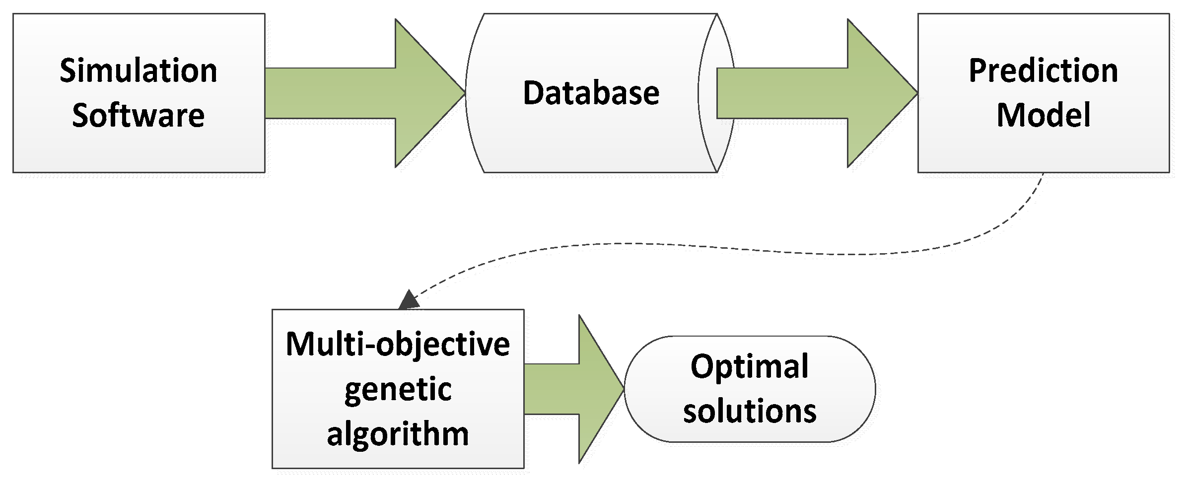20]. As parallel computing resources are not always available, the latter approach is adopted in this paper by developing prediction models to couple with genetic algorithms to find the optimal design solutions.

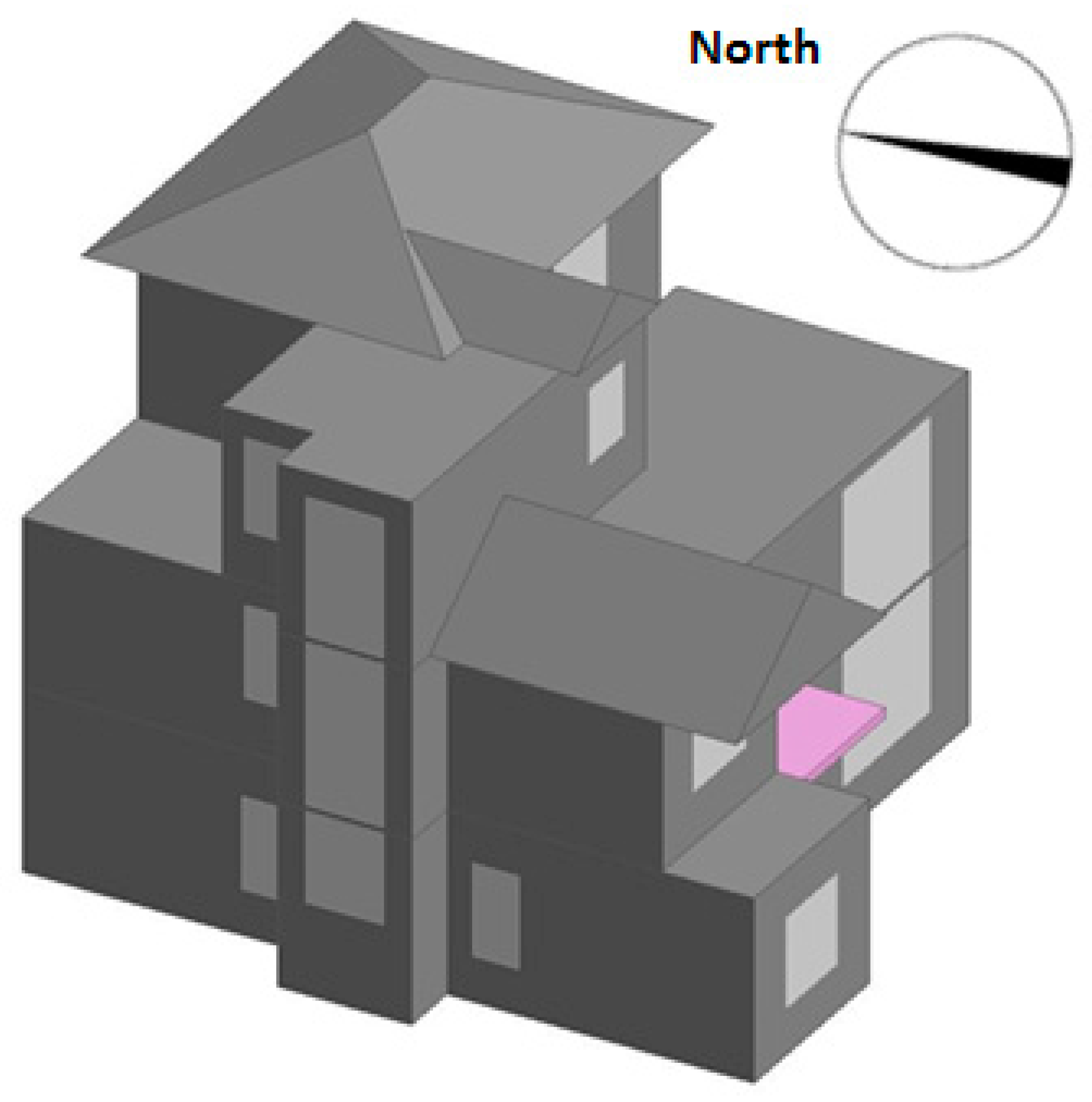
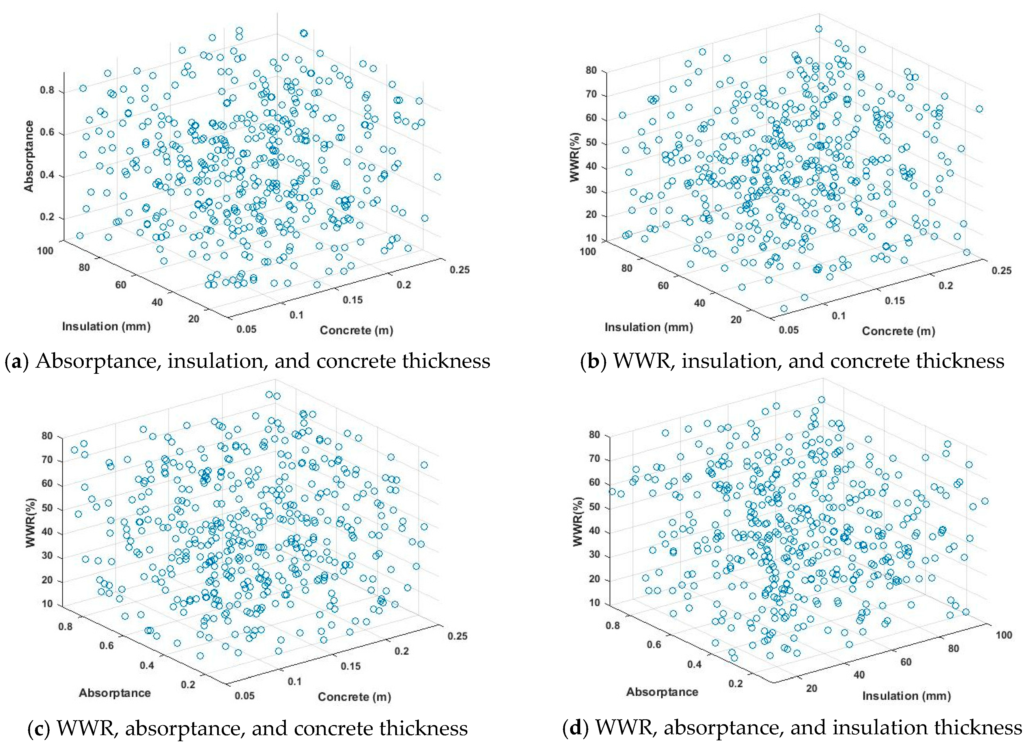
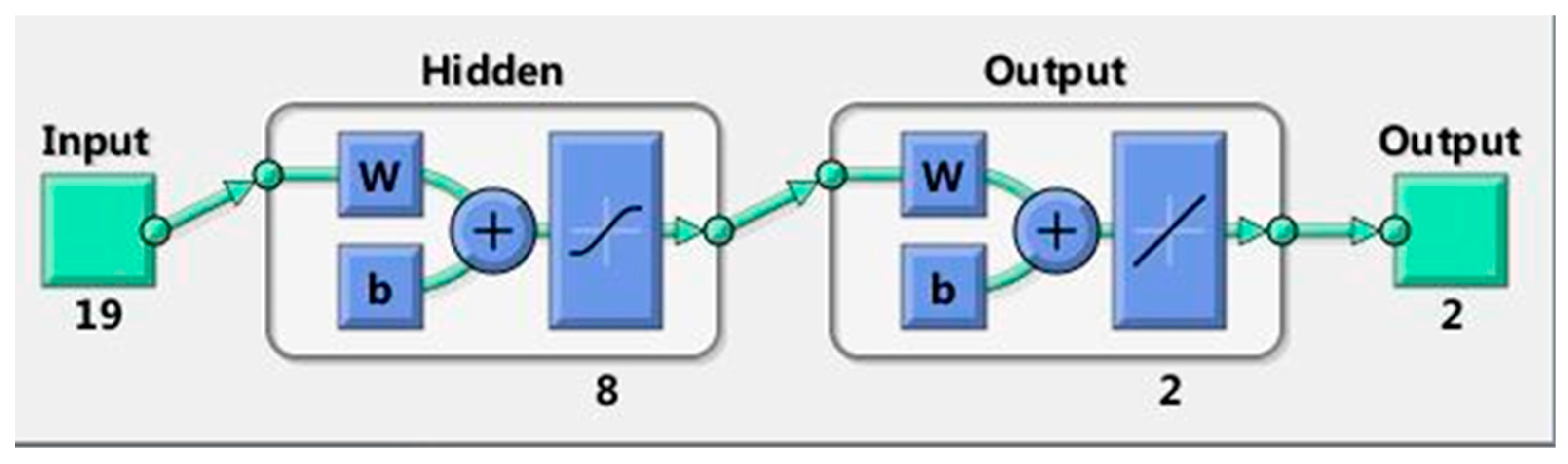
In this paper, different variables of thermal mass, insulation, absorbance of solar radiation are assigned for each exterior wall/roof, and the glazing ratios for each façade are considered separately. A total of 19 variables are considered, including five variables for concrete thickness, five variables for insulation thickness, five variables for the absorptance of solar radiation for each exterior walls/roof, and four variables for the window-to-wall ratio of each façade. In order to reduce the computation time, the Latin Hypercube Sampling Method is used to create the samples required to generate prediction models, and the commercial software, DesignBuilder (DesignBuilder Software Ltd, Stroud, Gloucestershire, UK) [36], is used to calculate the sub-hourly heating load, cooling load, and indoor air temperature to evaluate the thermal comfort condition. Two typical prediction models, multi-linear regression (MLR) model and an artificial neural network (ANN) model, are developed based on the sample data and coupled with a multi-objective genetic algorithm to find the optimal design solutions. The results from the two objective functions, namely, thermal load and annual discomfort degree hours, are also compared with the outcomes using the cooling load, heating load, summer discomfort degree hours, and winter discomfort degree hours as the objective functions for optimization.

The advantage of using the described method is that each component of the building envelope can be customized and the values of the building design parameters do not have to be the same if their orientations are different. The optimal model can be achieved by performing optimization with as many measures as possible, so that the least amount of materials can be determined to construct a building with a high indoor thermal comfort level and low thermal load. The accurate modeling can ensure utilizing the least amount of materials to achieve optimal building performance. Optimal usage of material for different building components can be selected to achieve a minimum thermal load and discomfort degree hours, which is different from traditional design, and can improve the quality of construction project. This is coincidence with 3D printing technology where the material for each component can be tailored. It is expected that advancement of 3D house printing technology will make it possible for wide application in design practice in the future.

2. Optimization Approach

2.1. Formulation of the Problem

2.1.1. Objective Functions to be Optimized

The following two objective functions are used in this study to find the optimal building design, and they are described as follows:

$${\mathrm{Min}\mathrm{f}}_1\left(\overline{\mathrm{x}}\right),{\mathrm{f}}_2\left(\overline{\mathrm{x}}\right),\overline{\mathrm{x}}=\left[{\mathrm{x}}_1,{\mathrm{x}}_2\cdots ,{\mathrm{x}}_{\mathrm{n}}\right].$$

(1)

The first objective function is the annual thermal load, which was also investigated by [5,37]. The total building thermal load, calculated by DesignBuilder (DesignBuilder Software Ltd., Stroud, Gloucestershire, UK) [36], was composed of a cooling load and heating load:

$${\mathrm{f}}_1\left(\overline{\mathrm{x}}\right)={\mathrm{Q}}_{\mathrm{C}}\left(\overline{\mathrm{x}}\right)+{\mathrm{Q}}_{\mathrm{H}}\left(\overline{\mathrm{x}}\right).$$

(2)

The second objective function is the total number of discomfort degree hours, which was proposed by Zhang et al. [38]. The total number of discomfort degree hours is composed of two parts. The first part is the cooling discomfort degree hours, which can be calculated as [37,38]:

$${\mathrm{I}}_{\mathrm{s}}\left(\overline{\mathrm{x}}\right)={{\displaystyle \sum }}_{\mathrm{i}=1}^{8760}\left({\mathrm{t}}_{\mathrm{i}}\left(\overline{\mathrm{x}}\right)-{\mathrm{t}}_{\mathrm{H}}\right)({\mathrm{if}\mathrm{t}}_{\mathrm{i}}\left(\overline{\mathrm{x}}\right)>{\mathrm{t}}_{\mathrm{H}}).$$

(3)

where ${\mathrm{t}}_{\mathrm{i}}\left(\overline{\mathrm{x}}\right)$ is the indoor air temperature at time i; and t_H is the higher limit temperature in the thermal comfort range, taken as 26 °C according to the energy efficient building design standard JGJ134-2010 [39].

The second part is the heating discomfort degree hours, which can be calculated as [38]:

$${\mathrm{I}}_{\mathrm{w}}\left(\overline{\mathrm{x}}\right)={{\displaystyle \sum }}_{\mathrm{i}=1}^{8760}\left({\mathrm{t}}_{\mathrm{L}}-{\mathrm{t}}_{\mathrm{i}}\left(\overline{\mathrm{x}}\right)\right)({\mathrm{if}\mathrm{t}}_{\mathrm{i}}\left(\overline{\mathrm{x}}\right)<{\mathrm{t}}_{\mathrm{L}}).$$

(4)

where t_L is the lower limit temperature in the thermal comfort range, taken as 18 °C according to JGJ134-2010 [39].

The total number of discomfort degree hours is then calculated as:

$${\mathrm{f}}_2\left(\overline{\mathrm{x}}\right)={\mathrm{I}}_{\mathrm{s}}\left(\overline{\mathrm{x}}\right)+{\mathrm{I}}_{\mathrm{w}}\left(\overline{\mathrm{x}}\right).$$

(5)

2.1.2. Base Model

The base building (see Figure 1) is a two-star green building, which was designed to meet the China Assessment Standard for Green Building GB-T50378 2014 [40]. It is a three-story building with a height of 11.77 m, floor area of 146.43 m², and a total construction area of 303.9 m². Exterior insulation and finish systems (EIFS) are adopted. The extruded polystyrene form board (XPS) is used for exterior wall and roof insulation. The double-layer low-E windows ensure enough daylighting, while effectively reducing the unwanted solar radiation in the daytime. Optimal building orientation of 15° west-to-south, as recommended by the building energy efficiency design standard JGJ134-2010 [39], is applied. The design helps to achieve thermal load reduction of 36% compared to a typical energy efficient building of the same size before further optimization is applied. The typical energy efficient building was built to meet the standard JGJ134-2010 [39] with K values of 0.974 W/m-K for the exterior walls, 0.592 W/m-K for the roof, and 3.835 W/m-K for the window, respectively. The thermal load of the energy efficient building is 36,301.50 kWh, while the one of the green building is 23,233.00 kWh.

Table 1. Values of the design parameters for the base building.

Design Parameter	Value of the Base Building	Requirements from JGJ134-2010 [39]
Floor area (m2)	146.43	-
Building height (m)	11.77	-
Total construction area (m2)	303.9	-
Shape factor	0.53	≤0.55
Heating temperature setpoint (°C)	18	18
Cooling temperature setpoint (°C)	26	26
K value of the external wall (W/m-K)	0.383	≤1.0
K value of the roof (W/m-K)	0.402	≤0.6
Window-to-wall ratio, East (%)	18	≤35
Window-to-wall ratio, South (%)	20	≤45
Window-to-wall ratio, West (%)	15	≤35
Window-to-wall ratio, North (%)	16	≤40
Building orientation	15° west-to-south	-

lists the values of design parameters of the base building and the requirements from the energy efficient building design standard JGJ134-2010 [39]. It can be found that the K values of the external walls/roof and window-to-wall ratio far exceed the requirements from JGJ134-2010 [39].

A total of 19 design variables are selected for study, which are concrete thickness, insulation thickness, and absorptance of solar radiation for each external wall/roof, and window-to-wall ratio for each façade.

Table 2. Variable types and value ranges.

Design Variable		Range	Value for Base Building
Concrete thickness (m)	East (x1)	[0.05, 0.25]	0.24
	South (x2)	[0.05, 0.25]	0.24
	West (x3)	[0.05, 0.25]	0.24
	North (x4)	[0.05, 0.25]	0.24
	Roof (x5)	[0.05, 0.25]	0.24
Insulation thickness (mm)	East (x6)	[10, 100]	50
	South (x7)	[10, 100]	50
	West (x8)	[10, 100]	50
	North (x9)	[10, 100]	50
	Roof (x10)	[10, 100]	60
Absorption of solar radiation	East (x11)	[0.1, 0.9]	0.7
	South (x12)	[0.1, 0.9]	0.7
	West (x13)	[0.1, 0.9]	0.7
	North (x14)	[0.1, 0.9]	0.7
	Roof (x15)	[0.1, 0.9]	0.7
Window-to-wall ratio (%)	East (x16)	[10, 80]	18
	South (x17)	[10, 80]	20
	West (x18)	[10, 80]	15
	North (x19)	[10, 80]	16

lists the variable types and value ranges.

The climatic information of Wuhan is listed in

Table 3. Climatic information.

City	Latitude (°)	Longitude (°)	HDD18 (°C·d)	CDD26 (°C·d)	Average OAT (°C)	Climatic Region
Wuhan	30.62	114.13	1501	283	16.7	Hot Summer & Cold Winter Region

.

2.2. Optimization Framework

The optimization framework of this study is summarized in Figure 2, and is divided into three steps. In the first step the simulation software obtained the thermal load and discomfort degree hours for a selected number of samples, which are generated based on the ranges of the 19 design variables as shown in Table 2. In the second step the samples from the database is used to develop two prediction models, the MLR model and the ANN model. In the third step, the MLR model and the ANN model are used to couple with a multi-objective genetic algorithm to find the optimal solutions. Finally, the results of the optimal solutions based on different prediction models and objective functions are compared and discussed.

3. Prediction Model

3.1. Creation of the Sample Dataset

The Latin Hypercube Sampling Method (LHSM) [41] was used to generate the distribution of the simulation parameters used for constructing the sampling database. The LHSM generates a near-random sample of parameter values and ensures that the ensemble of random numbers is representative of the real variability. McKay [41] determined that a sample of 2 × N sampling data is enough (where N is the number of variables). However, Conraud [42] and Magnier and Haghighat [20] found 22.5 × N sampling data is more appropriate to accurately sample the search space. In this study, a total of 450 cases were generated, which is slightly higher than the numbers recommended by Conraud [42] and Magnier and Haghighat [20]. Visualizations of selected design parameters from each of the four categories, x₁ for the thickness of concrete, x₆ for the insulation thickness, x₁₁ for the absorption of solar radiation, and x₁₆ for the window-to-wall ratio (WWR), are presented in Figure 3. It can be observed that the 19-dimensional spaces are well covered with the 450 samples.

All the simulation cases were run using DesignBuilder (DesignBuilder Software Ltd, Stroud, Gloucestershire, UK) with a time step of 30 min. It took around 45 days to create the 450 sample buildings and perform simulations using a desktop computer configured with an Intel i5 CPU @ 1.60 GHz with 4 GB of memory.

3.2. MLR Model

A multi-linear regression model is a very popular approach and was proved to be able to predict annual building energy consumption by Asadi et al. [43]. The regression model can be presented as:

$$\mathrm{f}\left(\overline{\mathrm{x}}\right)={\mathrm{a}}_0+{\displaystyle \sum }_{\mathrm{i}=1}^{\mathrm{n}}{\mathrm{a}}_{\mathrm{i}}{\mathrm{x}}_{\mathrm{i}}.$$

(6)

where a₀, a₁, ..., and a_n are the estimations of the regression parameters, based on the least-square method.

The regression model for the total building thermal load and discomfort degree hours can be presented as:

$$\begin{array}{l}{\mathrm{f}}_1\left(\overline{\mathrm{x}}\right)=23029.4+158.9\ast {\mathrm{x}}_1+242.6\ast {\mathrm{x}}_2+701.5\ast {\mathrm{x}}_3+238.8\ast {\mathrm{x}}_{24}+1284.1\ast {\mathrm{x}}_5-\\ 9.6\ast {\mathrm{x}}_6-10.99\ast {\mathrm{x}}_7-15.62\ast {\mathrm{x}}_8-11.15\ast {\mathrm{x}}_9-16.12\ast {\mathrm{x}}_{10}-2633.4\ast {\mathrm{x}}_{11}-\\ 2420.8\ast {\mathrm{x}}_{12}-3749.1\ast {\mathrm{x}}_{13}-3472.7\ast {\mathrm{x}}_{14}-4228.5\ast {\mathrm{x}}_{15}+101.4\ast {\mathrm{x}}_{16}+62.21\ast {\mathrm{x}}_{17}+\\ 125.0\ast {\mathrm{x}}_{18}+71.33\ast {\mathrm{x}}_{19}.\end{array}$$

(7)

$$\begin{array}{l}{\mathrm{f}}_2\left(\overline{\mathrm{x}}\right)=3649.3-4.85\ast {\mathrm{x}}_1+12.55\ast {\mathrm{x}}_2+42.38\ast {\mathrm{x}}_3+15.75\ast {\mathrm{x}}_{24}+118.6\ast {\mathrm{x}}_5-\\ 0.5732\ast {\mathrm{x}}_6-0.4843\ast {\mathrm{x}}_7-0.9149\ast {\mathrm{x}}_8-0.5462\ast {\mathrm{x}}_9-0.7036\ast {\mathrm{x}}_{10}-85.95\ast {\mathrm{x}}_{11}-\\ 112.9\ast {\mathrm{x}}_{12}-203.2\ast {\mathrm{x}}_{13}-139.7\ast {\mathrm{x}}_{14}-172.9\ast {\mathrm{x}}_{15}+11.06\ast {\mathrm{x}}_{16}+7.377\ast {\mathrm{x}}_{17}+\\ 10.94\ast {\mathrm{x}}_{18}+8.125\ast {\mathrm{x}}_{19}.\end{array}$$

(8)

The regressions between the target simulated outputs and MLR predictions are presented in Figure 4. Good agreements are found between the simulations and predictions, as the regression coefficients for both models are higher than 0.9889. A total of 405 (90%) sample data points were used for training and the remaining 45 (10%) sample data points were used for validation, which is the same as in Magnier and Haghighat [20]. For the thermal load model, the R² values for training and validation are 0.9840 and 0.9922, respectively. For the discomfort degree hour model, the R² values are 0.9763 and 0.9860, respectively.

3.3. ANN Model

ANN mimics the animal brain neural network behaviors in handling distributed parallel information. The ANN is interconnected with a number of joins (called neurons). Each join is connected with a number of inputs and outputs for information processing. The ANN learns the relationship between inputs and outputs through training data [44]. The ANN model was applied by Magnier and Haghighat [20] to predict the building thermal load and energy consumption with a maximum relative error of less than 10%.

A complete ANN model includes the inputs and corresponding weight values, thresholds, one or more hidden layers, and outputs. In this case, there are 19 inputs, one hidden layer, and one output layer. The number of nodes at the hidden layer is determined according to the following formulas [45]:

$$\mathrm{m}<\mathrm{a}-1.$$

(9)

$$\mathrm{m}<\sqrt{\left(\mathrm{a}+\mathrm{b}\right)}+\mathrm{c}.$$

(10)

$$\mathrm{m}={\log }_2\mathrm{a}$$

(11)

where m is the number of nodes at the hidden layer; a is the number of nodes at the input layer (equal to 19 in this study); b is the number of output nodes; and c is a constant, which is between 0 and 10. The optimal number of nodes in the hidden layer in this study is 8.

Figure 5 presents the diagram of the ANN model in this study. The maximum number of epochs is 200. The learning speed is 0.03, and the target error precision is 5 × 10⁻⁵. The number of sample data for training and for validation are 405 (90%) and 45 (10%), respectively.

The regressions between the target simulated outputs and MLR predictions are presented in Figure 6. Good agreements are found between the simulations and predictions with regression coefficients for both models close to 1.0. For the thermal load model, the R² values for training and validation are 0.9901 and 0.9962, respectively. For the discomfort degree hour model, the R² values are 0.9892 and 0.9966, respectively.

3.4. Comparisons on Different Prediction Models

The comparisons on the performance of the two prediction models are presented in

Table 4. Comparison on the performance of the four prediction models.

Method	Thermal Load			Discomfort Degree Hour
	Regression Coefficient	Standard Deviation (kWh)	Maximum Relative Error/Maximum Absolute Error (kWh)	Regression Coefficient	Standard Deviation (°C·h)	Maximum Relative Error/Maximum Absolute Error (°C·h)
MLR	0.992	514.183	7.01%/1930.72	0.989	61.689	6.91%/354.32
ANN	0.996	362.28	6.01%/1380.70	0.996	36.235	3.51%/145.05

. It can be found that both the regression coefficients are higher than 0.989, which indicates very good agreements between the simulation and prediction outcomes. The ANN models perform better with higher regression coefficients and lower standard deviations. It can also be found that the relative errors of the discomfort degree hour models are always lower than the thermal load models. The maximum errors for all the models are less than 8%.

4. Results and Discussion

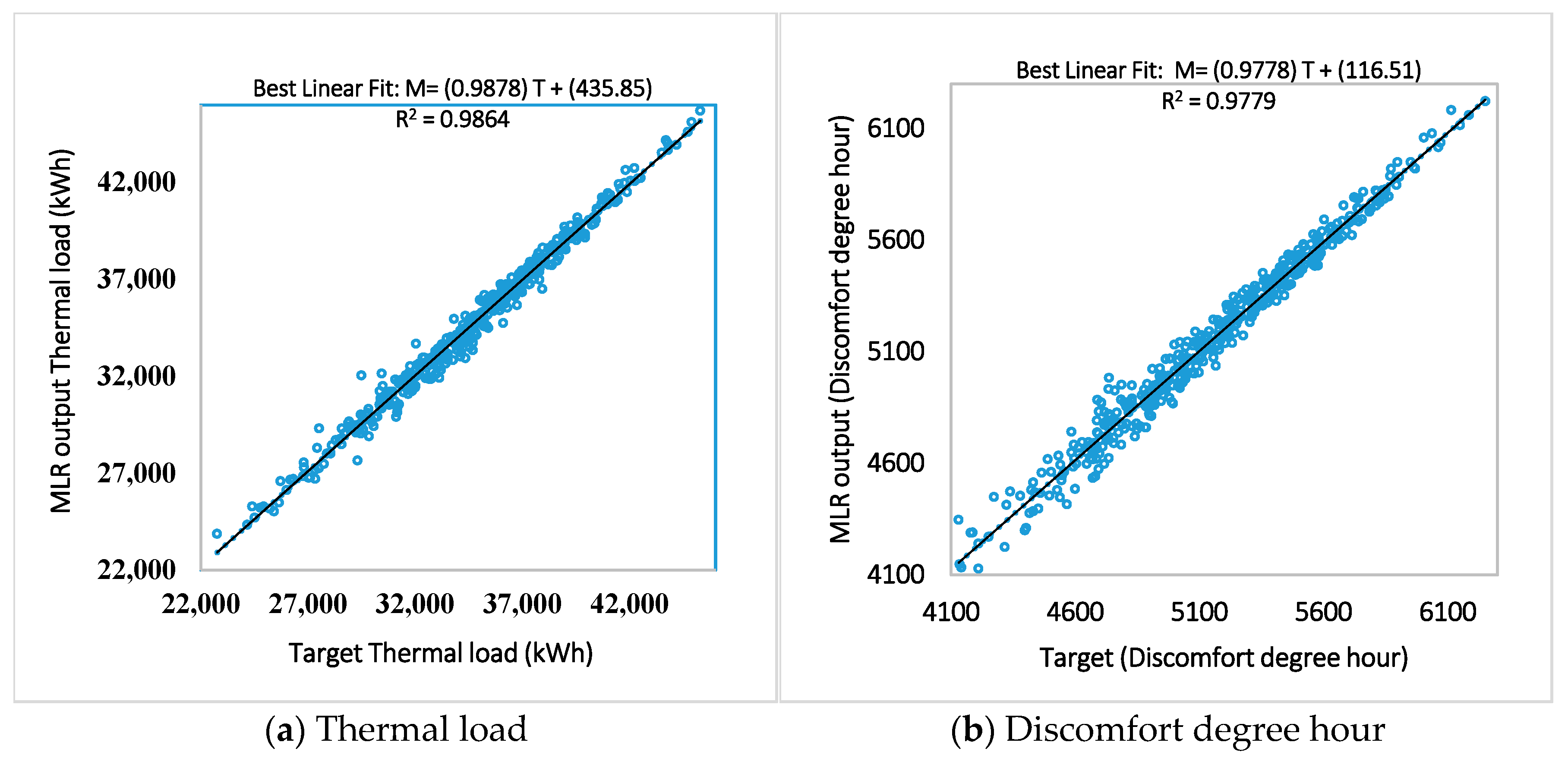
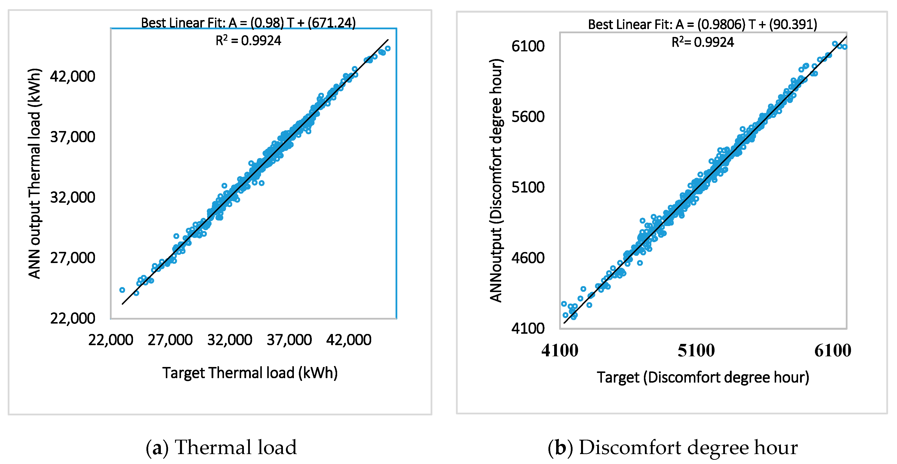
Since the prediction results from all models are in good agreement with simulation results, the ANN models and MLR models are coupled with a multi-objective genetic algorithm to find the optimal design solutions.

4.1. MLR with GA

The regression models (Equations (7) and (8)) are used as the fitness functions for a multi-objective optimization program using genetic algorithm developed in MATLAB. The constraints of the variables are presented as follows:

$$0.05\le {\mathrm{x}}_1,{\mathrm{x}}_2,{\mathrm{x}}_3,{\mathrm{x}}_4,{\mathrm{x}}_5\le 0.25$$

(12)

$$10\le {\mathrm{x}}_6,{\mathrm{x}}_7,{\mathrm{x}}_8,{\mathrm{x}}_9,{\mathrm{x}}_{10}\le 100$$

(13)

$$0.1\le {\mathrm{x}}_{11},{\mathrm{x}}_{12},{\mathrm{x}}_{13},{\mathrm{x}}_{14},{\mathrm{x}}_{15}\le 0.9$$

(14)

$$10\le {\mathrm{x}}_{16},{\mathrm{x}}_{17},{\mathrm{x}}_{18},{\mathrm{x}}_{19}\le 80$$

(15)

The program ran a number of times and each time came out with 1–4 Pareto front solutions when converged. A total of 45 solutions are obtained after 29 runs, after which the ranges of the outcomes for each design parameter stays unchanged. The maximum, minimum, median, average values, and standard deviations for the outcomes of the thermal load, number of discomfort degree hours, and each variable are summarized in

Table 5. Statistical values of the objective functions and design variables for MLRGA.

Item	Minimum	Maximum	Median	Average	Standard Deviation
Thermal load (kWh)	19,568.9	20,868.4	20,127.2	20,162.6	333.3
Ndis (°C·h)	3721.2	3822.1	3767.4	3766.7	23.8
x1 (m)	0.1553	0.2500	0.2466	0.2369	0.0221
x2 (m)	0.1564	0.2500	0.2428	0.2351	0.0230
x3 (m)	0.1947	0.2500	0.2498	0.2436	0.0111
x4 (m)	0.1775	0.2500	0.2493	0.2425	0.0155
x5 (m)	0.1751	0.2500	0.2500	0.2455	0.0126
x6 (mm)	31.5311	84.9766	52.9107	54.2241	13.5953
x7 (mm)	31.8788	74.5924	54.3463	54.5520	10.9994
x8 (mm)	42.5186	78.8962	63.8735	62.7198	9.6804
x9 (mm)	36.1280	79.5128	63.2697	58.2602	11.8191
x10 (mm)	37.0395	78.5900	63.0025	63.1980	9.4988
x11	0.1881	0.8366	0.4236	0.4398	0.1299
x12	0.2061	0.6710	0.3713	0.4325	0.1551
x13	0.1105	0.5694	0.2520	0.2656	0.0892
x14	0.1643	0.7348	0.3544	0.3960	0.1348
x15	0.1059	0.4254	0.1665	0.1865	0.0856
x16 (%)	10.4783	14.4398	11.2875	11.4404	0.8348
x17 (%)	10.5023	15.7129	12.1651	12.4202	1.4820
x18 (%)	10.3139	12.8394	11.1387	11.2782	0.6253
x19 (%)	10.5941	14.3469	11.7449	11.9172	0.8638

.

It is observed that the medians for the thickness of the concrete layer are higher than 0.24 m; for the insulation layer, are 52.9–63.9 mm; for the absorptance of solar radiation, are 0.167–0.424; and for the window-to-wall ratio, are 11.1–12.2%. There are differences on the values of design variables at different orientations, meaning the building can be adaptively designed to minimize the impact of outside weather conditions on the indoor environment.

The thermal load and number of discomfort degree hours for the best solution are 19,568.9 kWh and 3721.2 °C·h (19,000.4 kWh and 3755.4 °C·h from DesignBuilder (DesignBuilder Software Ltd., Stroud, Gloucestershire, UK)), while the ones for the base building are 23,233.0 kWh and 4840.0 °C·h. The reduction on the thermal load and number of discomfort degree hours are 18.2% and 22.4%, respectively. The relative errors on the predictions of the thermal load and discomfort degree hours are 2.99% and −0.91%, respectively.

4.2. ANN with GA

The ANN models developed in Section 3.3 are used as the fitness functions for the multi-objective optimization program, and the same constraints of the variables as in Section 4.1 are applied.

The program ran for a number of times and each time came out with 1–12 Pareto front solutions. A total of 44 solutions are obtained after 14 runs. The maximum, minimum, median, average values, and standard deviation for the outcomes of the thermal load, number of discomfort hours, and each variable are summarized in

Table 6. Statistical values of the objective functions and design variables for ANNGA.

Item	Minimum	Maximum	Median	Average	Standard Deviation
Thermal load (kWh)	18,938.4	20,694.8	20,017.3	19,986.7	342.4
Ndis (°C·h)	3592.8	3778.8	3738.1	3724.0	43.2
x1 (m)	0.1469	0.2499	0.2439	0.2273	0.0310
x2 (m)	0.1495	0.2500	0.2473	0.2343	0.0254
x3 (m)	0.1385	0.2500	0.2454	0.2233	0.0342
x4 (m)	0.1568	0.2500	0.2122	0.2113	0.0303
x5 (m)	0.1929	0.2500	0.2397	0.2297	0.0212
x6 (mm)	65.1231	81.3189	66.8935	69.2039	4.3327
x7 (mm)	35.9832	78.4017	58.5429	57.3585	12.2252
x8 (mm)	47.1732	81.7260	75.1834	70.6674	10.7494
x9 (mm)	45.8759	83.8319	68.4857	67.4576	9.2205
x10 (mm)	45.4588	83.8540	61.3895	64.6777	8.7629
x11	0.1397	0.5344	0.2390	0.2894	0.1280
x12	0.1180	0.7384	0.5406	0.4750	0.1364
x13	0.1111	0.5697	0.4214	0.3798	0.1432
x14	0.2277	0.7140	0.4712	0.4468	0.1258
x15	0.1069	0.5553	0.1944	0.2312	0.1167
x16 (%)	10.6752	13.4761	12.1307	12.4271	0.8153
x17 (%)	12.0535	18.2364	15.4413	15.7119	2.0794
x18 (%)	10.9451	14.7791	12.2079	12.4518	0.9828
x19 (%)	11.7572	14.9198	13.8030	13.7202	1.0660

.

It is observed that the medians for the thickness of the concrete layer are higher than 0.21 m, for the insulation layer are 58.5–75.2 mm, for the absorbance of solar radiation are 0.194–0.5406, and for the window-to-wall ratio are 12.1–15.4%.

The thermal load and number of discomfort degree hours for the best solution are 18,938.4kWh and 3592.8 °C·h (19,276.63 kWh and 3773.5 °C·h from DesignBuilder (DesignBuilder Software Ltd., Stroud, Gloucestershire, UK)). The reduction on the thermal load and number of discomfort degree hours are 17.0% and 22.2%, respectively. The relative errors on the predictions of the thermal load and discomfort degree hours are 1.75% and 4.76%, respectively.

4.3. Optimization with Different Combinations of Parameters

The ANNGA approach is applied for optimization on different combinations of parameters. The results on the optimization are presented in

Table 7. Comparison on the optimal solutions using different combinations of design parameters.

Optimization Parameter	Thermal Load	Increase in Thermal	Discomfort Degree Hours	Increase In Discomfort Degree Hours
	(kWh)	Load (%)	(°C·h)	(%)
1	23,795.0 *	25.6%	4087.6	13.8%
2	21,194.8	11.9%	3861.6	7.5%
3	22,271.7	17.6%	3947.2	9.9%
4	21,810.9	15.2%	3889.3	8.3%
1&2	21,159.9	11.7%	3856.4	7.3%
1&3	22,238.5	17.4%	3943.4	9.8%
1&4	21,698.8	14.6%	3883.7	8.1%
2&3	20,346.4	7.4%	3768.3	4.9%
2&4	21,096.2	11.4%	3836.8	6.8%
3&4	20,572.4	8.6%	3780.5	5.2%
1&2&3	20,273.3	7.0%	3761.1	4.7%
1&2&4	21,064.6	11.2%	3832.9	6.7%
1&3&4	20,538.2	8.4%	3775.8	5.1%
2&3&4	19,780.7	4.4%	3674.6	2.3%
1&2&3&4	18,938.4	0.0%	3592.8	0.0%

* The prediction on the thermal load of the base case building is 24,000.9 kWh. Through optimization, only 46.8% of concrete for the east wall is needed as compared to the base building. It is found that when the insulation thickness is higher than 60 mm, the reduction on thermal load and discomfort degree hours by increasing the insulation thickness is very small (less than a 2% reduction on thermal load per 10 mm increase in insulation thickness and no reduction when insulation thickness increases to 200 mm). The thickness of insulation needs to be at least 200 mm (about four times the thickness of the optimal solution) to reduce the same thermal load as the optimal solution. However, the discomfort degree hour stays at 3831.3 °C·h. The thermal load and discomfort degree hours do not decrease with further increase in the insulation thickness. The cost of changing all this variables to get the optimized solution is ¥23,686.911 less than by simply increasing the thickness of insulation to 200 mm. In addition, the increase of wall thickness will lead to less internal space for same floor area, which is not a preferred option.

, where “1” refers to the concrete thickness; “2” refers to the insulation thickness; “3” refers to the absorptance of solar radiation; and “4” refers to the window-to-wall ratio. The results clearly show that when one more group of parameters is added, there is a further improvement on the building performance.

4.4. Optimization with Four Objective Functions

The ANN models for the total hourly cooling load (Q_C), heating load (Q_H), discomfort heating degree hours (I_W), and cooling degree hours (I_S) are developed and used as fitness functions for the multi-objective optimization program. A total of 70 Pareto front solutions are generated and summarized as in

Table 8. Pareto front solutions characteristic for four objective functions.

	Thermal Load	Ndis	Cooling Load	Heating Load	Discomfort Heating Degree Hours	Discomfort Cooling Degree Hours
	(kWh)	(°C·h)	(kWh)	(kWh)	(°C·h)	(°C·h)
Minimum	19,518.5	3691.6	12,078.5	3810.3	2117.3	1031.5
Maximum	35,841.7	5488.9	31,015.7	9479.6	4457.4	1644.9
Median	23,603.2	4303.9	18,605.5	5041.4	3017.7	1288.2
Average	25,028.5	4389.8	19,482.3	5546.2	3091.5	1298.3
Standard deviation	4590.0	545.0	5753.6	1491.8	716.5	176.3

Notes: minimum cooling load, and minimum heating load might not happen at the same time; similarly, minimum discomfort heating degree hours and minimum discomfort cooling degree hours might not occur at the same time.

.

It can be found that although a few solutions can achieve total thermal load and number of discomfort degree hours as low as the ones presented in Section 4.1 and Section 4.2, the average values of which are much higher, indicating lower optimization performance. Therefore, two objective functions are sufficient for optimization purpose.

5. Conclusions

In this paper, an MLR model and ANN model are developed to predict the building thermal load and the number of discomfort degree hours considering the variable thermal mass, insulation, absorptance of solar radiation, and glazing ratio. The MLR models and ANN models are coupled with a multi-objective genetic optimization algorithm to minimize the building thermal load and improve the thermal comfort for a very energy-efficient two-star green building in China. Finally, optimization with four objective functions is also performed. The following conclusions can be made:

(1)

The ANN models perform better than the MLR models in terms of regression coefficients, standard deviations, and absolute errors. The relative errors of the discomfort degree hour models are always lower than the thermal load models.

(2)

When used as fitness functions for GA to obtain the optimal building design solutions, the MLR model and ANN model have similar performances.

(3)

The optimal solutions prefer concrete layer with median thickness higher than 0.21 m; insulation layer, 52.9–75.2 mm; absorbance of solar radiation, 0.167–0.5406; and window-to-wall ratio, 11.1–15.4%.

(4)

The optimal design solutions help to reduce the thermal load and the number of discomfort hours of the two-star green building by up to 18.2% and 22.4%, respectively.

(5)

The two objective functions are better than the four objective functions to perform the optimization on thermal load and thermal comfort.

References

1. IEA. 2015. Buildings Energy Use in China, Transforming Construction and Influencing Consumption to 2050. Available online: http://www.iea.org (assessed on 5 October 2017).
2. EAI. 2017. How Much Energy Is Consumed in U.S. Residential and Commercial Buildings? Available online: https://www.eia.gov/tools/faqs/faq.php?id=86&t=1 (assessed on 5 October 2017).
3. Filippin, C.; Larsen, S.F.; Beascochea, A.; Lesino, G. Response of conventional and energy-saving buildings to design and human dependent factors. Sol. Energy 2005, 78, 455–470. [Google Scholar] [CrossRef]
4. Badescu, V.; Laaser, N.; Crutescu, R.; Crutescu, M.; Dobrovicescu, A.; Tsatsaronis, G. Modeling, validation and time-dependent simulation of the first large passive building in Romania. Renew. Energy 2011, 36, 142–157. [Google Scholar] [CrossRef]
5. Gong, X.; Akashi, Y.; Sumiyoshi, D. Optimization of passive design measures for residential buildings in different Chinese areas. Build. Environ. 2012, 58, 46–57. [Google Scholar] [CrossRef]
6. Zhu, Y. Built Environment, 4th ed.; China Architectural Engineering Industrial Publishing Press: Beijing, China, 2016. [Google Scholar]
7. Delgarm, N.; Sajadi, B.; Delgarm, S. Multi-objective optimization of building energy performance and indoor thermal comfort: A new method using artificial bee colony (ABC). Energy Build. 2016, 131, 42–53. [Google Scholar] [CrossRef]
8. Ascione, F.; Bianco, N.; De Stasio, C.; Mauro, G.M.; Vanoli, G.P. A new comprehensive approach for cost-optimal building design integrated with the multi-objective model predictive control of HVAC systems. Sustain. Cities Soc. 2017, 31, 136–150. [Google Scholar] [CrossRef]
9. Brea, F.; Fachinotti, V.D. A computational multi-objective optimization method to improve energy efficiency and thermal comfort in dwelling. Energy Build. 2017, 154, 283–294. [Google Scholar] [CrossRef]
10. Brea, F.; Silva, A.S.; Ghisi, E.; Fachinotti, V.D. Residential building design optimisation using sensitivity analysis and genetic algorithm. Energy Build. 2016, 133, 853–866. [Google Scholar] [CrossRef]
11. Ascione, F.; Bianco, N.; De Stasio, C.; Mauro, G.M.; Vanoli, G.P. A new methodology for cost-optimal analysis by means of the multi-objective optimization of building energy performance. Energy Build. 2015, 88, 78–90. [Google Scholar] [CrossRef]
12. Ihm, P.; Krarti, M. Design optimization of energy efficient residential buildings in Tunisia. Build. Environ. 2012, 58, 81–90. [Google Scholar] [CrossRef]
13. Evins, R. Multi-level optimization of building design, energy system sizing and operation. Energy 2015, 90, 1775–1789. [Google Scholar] [CrossRef]
14. Krarti, M.; Deneuville, A. Comparative evaluation of optimal energy efficiency designs for French and US office buildings. Energy Build. 2015, 93, 332–344. [Google Scholar] [CrossRef]
15. Xu, J.; Kim, J.; Hong, H.; Koo, J. A systematic approach for energy efficient building design factors optimization. Energy Build. 2015, 89, 87–96. [Google Scholar] [CrossRef]
16. Delgarm, N.; Sajadi, B.; Delgarm, S.; Kowsary, F. A novel approach for the simulation-based optimization of the buildings energy consumption using NSGA-II: Case study in Iran. Energy Build. 2016, 127, 552–560. [Google Scholar] [CrossRef]
17. Yong, S.; Kim, J.; Gim, Y.; Kim, J.; Cho, J.; Hong, H.; Baik, Y.; Koo, J. Impacts of building envelope design factors upon energy loads and their optimization in US standard climate zones using experimental design. Energy Build. 2017, 141, 1–15. [Google Scholar] [CrossRef]
18. Caldas, L.G.; Norford, L.K. A design optimization tool based on a genetic algorithm. Automat. Constr. 2002, 11, 173–184. [Google Scholar] [CrossRef]
19. Wang, W.; Zmeureanu, R.; Rivard, H. Applying multi-objective genetic algorithms in green building design optimization. Build. Environ. 2005, 40, 1512–1525. [Google Scholar] [CrossRef]
20. Magnier, L.; Haghighat, F. Multiobjective optimization of building design using TRNSYS simulations, genetic algorithm, and Artificial Neural Network. Build. Environ. 2010, 45, 739–746. [Google Scholar] [CrossRef]
21. Bichiou, Y.; Krarti, M. Optimization of envelope and HVAC systems selection for residential buildings. Energy Build. 2011, 43, 3373–3382. [Google Scholar] [CrossRef]
22. Ramallo-González, A.P.; Coley, D.A. Using self-adaptive optimisation methods to perform sequential optimisation for low-energy building design. Energy Build. 2014, 81, 18–29. [Google Scholar] [CrossRef] [Green Version]
23. Yu, W.; Li, B.; Ji, H.; Zhang, M.; Wang, D. Application of multi-objective genetic algorithm to optimize energy efficiency and thermal comfort in building design. Energy Build. 2015, 88, 135–143. [Google Scholar] [CrossRef]
24. Liu, S.; Meng, X.; Tam, C. Building information modeling based building design optimization for sustainability. Energy Build. 2015, 105, 139–153. [Google Scholar] [CrossRef]
25. Lin, Y.; Tsai, K.; Lin, M.; Yang, M. Design optimization of office building envelope configurations for energy conservation. Appl. Energy 2016, 171, 336–346. [Google Scholar] [CrossRef]
26. Azari, R.; Garshasbi, S.; Amini, P.; Rashed-Ali, H.; Mohammadi, Y. Multi-objective optimization of building envelope design for life cycle environmental performance. Energy Build. 2016, 126, 524–534. [Google Scholar] [CrossRef]
27. Zhang, A.; Bokel, R.; Dobbelsteen, A.V.D.; Sun, Y.; Huang, Q.; Zhang, Q. Optimization of thermal and daylight performance of school buildings based on a multi-objective genetic algorithm in the cold climate of China. Energy Build. 2017, 139, 371–384. [Google Scholar] [CrossRef]
28. Bambrook, S.M.; Sproul, A.B.; Jaco, D. Design optimisation for a low energy home in Sydney. Energy Build. 2011, 43, 1702–1711. [Google Scholar] [CrossRef]
29. Baglivo, C.; Congedo, P.M.; Fazio, A. Multi-criteria optimization analysis of external walls according to ITACA protocol for zero energy buildings in the mediterranean climate. Build. Environ. 2014, 82, 467–480. [Google Scholar] [CrossRef]
30. Hamdy, M.; Hasan, A.; Siren, K. Applying a multi-objective optimization approach for Design of low-emission cost-effective dwellings. Build. Environ. 2011, 46, 109–123. [Google Scholar] [CrossRef]
31. Romani, Z.; Draoui, A.; Allard, F. Metamodeling the heating and cooling energy needs and simultaneous building envelope optimization for low energy building design in Morocco. Energy Build. 2015, 102, 139–148. [Google Scholar] [CrossRef]
32. Carreras, J.; Boer, D.; Cabeza, L.F.; Jiménezc, L.; Guillén-Gosálbez, G. Eco-costs evaluation for the optimal design of buildings with lower environmental impact. Energy Build. 2016, 119, 189–199. [Google Scholar] [CrossRef]
33. Pal, S.K.; Takano, A.; Alanne, K.; Siren, K. A life cycle approach to optimizing carbon footprint and costs of a residential building. Build. Environ. 2017, 123, 146–162. [Google Scholar] [CrossRef]
34. Shi, X. Design optimization of insulation usage and space conditioning load using energy simulation and genetic algorithm. Energy 2011, 36, 1659–1667. [Google Scholar] [CrossRef]
35. Yang, C.; Li, H.; Rezgui, Y.; Petri, I.; Yuce, B.; Chen, B.; Jayan, B. High throughput computing based distributed genetic algorithm for building energy consumption optimization. Energy Build. 2014, 76, 92–101. [Google Scholar] [CrossRef]
36. Design Builder. 2016. Available online: http://www.designbuilder.co.uk/ (accessed on 1 September 2016).
37. Gossard, D.; Lartigue, B.; Thellier, F. Multi-objective optimization of a building envelope for thermal performance using genetic algorithms and artificial neural network. Energy Build. 2013, 67, 253–260. [Google Scholar] [CrossRef]
38. Zhang, Y.; Lin, K.; Zhang, Q.; Di, H. Ideal thermophysical properties for free-cooling (or heating) buildings with constant thermal physical property material. Energy Build. 2006, 38, 1164–1170. [Google Scholar] [CrossRef]
39. Ministry of Housing and Urban-Rural Development of the People’s Republic of China (MOHURD) JGJ134-2010. Residential Building Energy Efficiency Design Standard for Hot Summer/Cold Winter Region; China Architectural Engineering Industrial Publishing Press: Beijing, China, 2010. [Google Scholar]
40. GB-T50378 2014. Ministry of Housing and Urban-Rural Construction of the People’s Republic of China. Assessment Standard for Green Building; China Architectural Engineering Industrial Publishing Press: Beijing, China, 2014. [Google Scholar]
41. McKay, M.D. Sensitivity Arid Uncertainty Analysis Using a Statistical Sample of Input Values, Uncertainty Analysis; CRC Press: Boca Raton, FL, USA, 1988; pp. 145–186. [Google Scholar]
42. Conraud, J. A Methodology for the Optimization of Building Energy, Thermal, and Visual Performance. Master’s Thesis, Concordia University, Montreal, QC, Canada, 2008. [Google Scholar]
43. Asadi, S.; Amiri, S.S.; Mottahedi, M. On the development of multi-linear regression analysis to assess energy consumption in the early stages of building design. Energy Build. 2014, 85, 246–255. [Google Scholar] [CrossRef]
44. Kalogirou, S.A. Applications of artificial neural networks in energy systems. Energy Convers. Manag. 1999, 40, 1073–1087. [Google Scholar] [CrossRef]
45. Wang, X.; Shi, F.; Yu, L.; Li, Y. Analysis on 43 Neural Network Application Cases Using MATLAB; Beijing University of Aeronautics and Astronautics Publishing Press: Beijing, China, 2013. [Google Scholar]
Figure 1. Overview of the base building.
Sustainability 10 00336 g001
Figure 2. Optimization framework.
Sustainability 10 00336 g002
Figure 3. Visualizations of selected design parameters.
Sustainability 10 00336 g003
Figure 4. Regression between MLR outputs and simulated targets.
Sustainability 10 00336 g004
Figure 5. ANN model diagram.
Sustainability 10 00336 g005
Figure 6. Regression between ANN outputs and simulated targets.
Sustainability 10 00336 g006