Article

Spatial Spillover and the Influencing Factors Relating to Provincial Carbon Emissions in China Based on the Spatial Panel Data Model

1
School of Economics, Central University of Finance and Economics, Beijing 100081, China
2
School of Business Administration, Northeastern University, Shenyang 110819, China
3
College of Science and Technology, Shenyang Polytechnic College, Shenyang 110021, China
4
Department of Engineering Technology, Dalian Maple Leaf College of Technology, Dalian 116036, China
*
Author to whom correspondence should be addressed.
Sustainability 2018, 10(12), 4739; https://doi.org/10.3390/su10124739
Submission received: 20 September 2018 / Revised: 18 November 2018 / Accepted: 5 December 2018 / Published: 12 December 2018

Abstract

:
From the perspective of spatial geography, this paper verifies the spatial dependence of China’s provincial carbon emissions. The contribution of impact factors with different fields of view to carbon emissions’ growth is estimated based on the spatial panel data model, t. The study found that during 2000–2015, China’s energy-related carbon emissions in the provinces were dependent on the spatial, and the spatial spillover effect of carbon emissions and its influencing factors in the neighboring provinces are obvious. It was also found that economic growth, industrial structure, financial development, and urbanization rates are positive, and the effect of the population and technological progress on reducing carbon emissions is significant. The effect of source price, export dependence, and fiscal decentralization on carbon emissions’ growth did not pass a significance test. In the formulation of carbon emission-related policies and development plans, the government must consider the effect of the influencing factors affecting the carbon emissions in the adjacent area and combine the carbon emissions and spatial spillover effect of the related factors in order to reduce carbon emissions in the time dimension and the spatial dimension of China as a whole.

1. Introduction

The problem of carbon emissions and its influencing factors has become an important subject in relation to climate problems; China’s carbon emissions problems are also in a very complex and uncertain environment. The existence and development of carbon emission problems will affect the economic development of the whole country. The methods of reducing carbon emissions are divided into two dimensions: one focusing on the internal factors, such as population and economic growth, and the other one on the external factors, such as carbon spillover. China is the largest developing country and has many provinces and regions, and the characteristics of economic development in the different regions lead to relative difficulty in controlling carbon emissions. In view of these problems, it is of great significance to take corresponding measures to coordinate the development of regional low-carbon economies and achieve an overall low-carbon economy. The existing carbon emission problems are mainly analyzed in relation to several factors at the national level; representative research, such as the work by Christidou, examines the stationarity of carbon emissions per capita and finds strong evidence that the per capita carbon dioxide emissions over the last 150 years are stationary [1]. Dergiades tested two hypotheses derived from the anthropogenic theory of climate change, and the results indicate that physical mechanisms underlie the theory of anthropogenic climate change [2]. Libo Wu and other scholars used the logarithmic mean Divisia index decomposition method to study the relationship between the per capita carbon dioxide emissions of different regions in China, as well as the influencing factors affecting energy consumption [3,4,5]. Additionally, Li Na and other scholars studied the influencing factors affecting carbon emissions using grey relational theories [6,7]. Research on the influencing factors affecting carbon emissions began at the beginning of the 21st century, and most of it applied the research methods of foreign scholars to analyze China’s energy consumption and carbon emissions. Existing research methods on carbon emissions and their influencing factors mainly use the decomposition method to decompose China’s carbon emissions into population, energy consumption intensity, per capita GDP, and other factors. Some scholars used the Laplace index decomposition method to analyze China’s carbon emissions with respect to population, energy consumption intensity, per capita GDP, energy consumption, and other factors [8,9]. Wu, Kaneko, and other scholars decomposed the influencing factors affecting carbon emissions by means of the logarithmic mean decomposition and studied the impact of factors such as per capita carbon dioxide emissions, energy consumption structure, energy efficiency, and energy intensity in China. The empirical results show that optimizing the energy consumption structure and industrial structure and improving energy utilization efficiency are all important. The contribution of the rate of economic growth to per capita carbon dioxide emissions will increase exponentially [3]. Other researchers studied the influencing factors affecting carbon emissions in Beijing and Shanghai from 1985 to 1998 using the Dean decomposition method [10]. Li decomposed and analyzed the changes of industrial carbon dioxide emission intensity in Xinjiang from 1994 to 2007 [11]. Zhao Aiwen and Li Dong analyzed the data of per capita carbon emissions and per capita GDP by means of the logarithmic mean decomposition method [12]. The results show that the increase of per capita GDP is the main driving factor behind the increase of per capita carbon emissions, and the decrease of energy consumption per unit GDP is the main factor restraining the increase of per capita carbon emissions. Fan, Luo et al. analyzed the factors affecting carbon dioxide emissions in China’s chemical industry from 1996 to 2007 by means of the logarithmic mean decomposition method [13]. The results show that economic activity and energy intensity decline are the two most important factors affecting carbon dioxide emissions in the chemical industry. Tension and Lei et al. used the logarithmic average Di’s method to decompose the total carbon emissions in Xinjiang, and quantitatively analyzed the effect of different stages of carbon emissions in Xinjiang on overall carbon emissions [14]. The results show that economic growth is a major factor affecting the rise of carbon emissions. Song used the two-stage logarithmic mean decomposition method to analyze the factors affecting China’s carbon emissions from 1990 to 2005 and reached the same conclusion [15].
Another major research method is the Kaya identity method, proposed by Yoichi Kaya, a famous foreign scholar. Based on the Kaya equation, He and Zhang constructed a decomposition model of influencing factors affecting carbon emissions in the iron and steel industries and discussed the equilibrium relationship between carbon emissions and influencing factors by the cointegration method [16]. According to the conclusion of the quantitative analysis, the paper puts forward relevant countermeasures and suggestions in relation to three aspects: controlling the growth rate of China’s iron and steel industries, increasing the proportion of clean energy, and carrying out technological innovation. Zhubased on the Kaya identity analysis and a decomposition analysis of China’s 1980–2007 carbon emissions, concluded that China’s carbon emissions increase is mainly driven by economic expansion [17].
Li and Li used panel data to analyze the relationship between carbon dioxide emissions and population, economy, and technology in different regions [18]. The results show that there are obvious differences in carbon dioxide emissions in different regions, and the differences are constantly increasing. Similarly, rapid economic growth is the most important driving factor behind the increase of carbon dioxide emissions in various regions. Based on the improved STIRPAT model, He and Zhang found that R&D intensity is not the main factor affecting emissions; rather, carbon dioxide emissions are a dynamic adjustment process with an obvious lag effect, and the government’s energy-saving and emission-reduction policies are conducive to reducing emissions [19]. Zhu, Peng et al. used the extended STIRPAT model with the ridge regression method to analyze the impact of population and technology on carbon emissions [20]. The results show that technological progress has limited explanatory power for China’s emissions at this stage, so the potential of reducing carbon emissions through technological progress in the future is huge.
It can be seen that some valuable research results have been obtained on China’s carbon emissions by scholars at home and abroad. However, only a few influencing factors affecting carbon emissions have been considered, there is a lack of comprehensive consideration of the influencing factors affecting carbon emissions. The method of intersequence analysis is useful when there is a lack of spatial panel data analysis. In this paper, spatial statistics and spatial econometric models are used to empirically analyze the effects of different factors on carbon emissions from the provinces of China and detect the spatial dependence of carbon emissions and the spatial mechanism of carbon emissions. This study distinguishes the pattern of carbon emission clusters in local areas and investigates the LISA index for the period 2000 to 2015 and seeks to thoroughly consider the main influencing factors contributing to the carbon emissions in the provinces of China.
The main innovation in this paper is the analysis of the carbon clusters in local areas with the LISA index in China, extended to nine influencing factors of carbon emissions by conducting further research; in addition, our study takes into account the spatial factor.

2. Materials and Methodology

2.1. Model

In the 1970s, Professors Ehrlich and Commoner of Stanford established IPAT formulas for assessing environmental pressures and studied the mechanisms by which population, economic growth, and technological progress influence carbon emissions. STIRPAT is the modification and extension of the IPAT model, which can overcome the deficiency of the IPAT model assumption. The representative studies of the STIRPAT model are those of He, Zhuand other scholars, who used the STIRPAT model to study the influence of population, technology, and other factors on the environmental problem [21,22,23]. In this paper, the STIRPAT model is used to construct a carbon emission model in order to estimate the elastic coefficient of the impact factors affecting carbon emissions and to test the spillover effects of carbon emissions. The specific expressions of the IPAT model are as follows [20,24]:
Im p a c t ( I ) = P o p u l a t i o n ( p ) × A f f l u e n c e ( A ) × T e c h o log y ( T )
where I represents the environmental load, P represents the population factor, A represents levels of wealth, and T represents the technical level. The STIRPAT model is an extended stochastic model that evaluates the environmental impact through the three independent variables of population, property, and technology, and the relationship between the dependent variables.
I = a × P b × A c × T d × e
where a is the constant of the model; b, c, and d are all exponential terms; and e is the error term. When a, b, c, and d are all 1, the STIRPAT model is reduced to the IPAT model.
Based on the STIRPAT model, this paper constructs an econometric model for the relationship between carbon emissions and the influencing factors:
I = a × P b × A c × T d × S e × F f × E g × E X h × U k × F D l + ε
where I, P, A, T, S, F, E, EX, U and FD represent carbon emissions, population, economic growth, technological progress, industrial structure, financial development, energy price, international trade, urbanization rate, and fiscal decentralization, respectively, and b, c, d, e, f, g, h, k, and l are all model parameters.
The logarithm of the carbon emission function is changed to an empirical analysis model:
l n I i = l n a + b l n P i + c l n A i + d l n T i + e l n S i + f l n F i + g l n E i + h l n E X i + k l n U i + l l n F D i + ε i
where a is a constant, b represents the elastic coefficient of population growth causing carbon emissions in the i region, c represents the elastic coefficient of economic growth, d represents the elastic coefficient of technological progress, e indicates the elastic coefficient of industrial structure, f indicates the elastic coefficient of financial development, g represents the elastic coefficient of energy price, h represents the elastic coefficient of international trade, k is the coefficient of elasticity of the urbanization rate, and l represents the elastic coefficient of fiscal decentralization, which represents a stochastic term.

2.2. Data

In this paper, referring to the existing literature [25,26,27] and the carbon emission measurement methods of the IPCC [28], CDIAC, and other international organizations, the carbon emission calculation formula is determined:
I i t = j = 1 n ( E i j t × E j × E F j )  
where:
I i t : The total amount of carbon emissions in the ith province for the year t; (i = 1, …, 30, t = 2000, …, 2015).
E i j t : The total energy consumption of j in year t.
E j : The conversion standard coal coefficient of the jth type of energy.
EFj: The carbon emission coefficient of the jth type of energy.
j: Type of energy.
The carbon emissions of different energy sources were calculated using their respective carbon emission coefficients. The carbon emission coefficients used by different countries and studies are different (see Table 1). Because each kind of energy consumption in the “China Energy Statistics Yearbook” is the physical quantity, this research first determines the conversion standard coal coefficient according to the “China Energy Statistics Yearbook”—that is, 1 kg raw coal equates to 0.7143 kg standard coal, 1 m3 natural gas equates to 1.3300 kg standard coal, and 1 kg crude oil equates to 1.4286 kg standard coal—which converts the different energy sources into standard coal, and the carbon emission coefficient recommended by the United States Department of Energy and the carbon emissions of 30 provinces of China for the period 2000–2015 were calculated (excluding Hong Kong, Macao, Taiwan, and Tibet due to lack of data).
The research in the carbon emission-related literature, the impact factors affecting carbon emissions from domestic and foreign scholars, and the availability and integrity of the data should be considered in respect to studies and the actual situation in China. The research on the influencing factors affecting carbon emissions, such as those of Weber and Wang [7,29], have investigated the different impacts of carbon emissions based on the input–output model. Based on static and dynamic panel models, Li found that international trade has increased China’s carbon dioxide emissions and carbon emissions intensity, which has had a serious negative impact on the environment. Population size, economic development, and technological progress are the core elements of the study of carbon emissions. Birdsall et al. believe that the increase in population will lead to an increase in energy consumption, resulting in relatively large carbon emissions, and that population growth will increase the damage to the ecological environment [30]. Knapp et al. believe that population growth is the main driving force behind global carbon emissions, and the increase of the global population is also an important reason for the rapid increase of global carbon emissions [31]. Tan Dan et al. analyzed the carbon emissions and industrial development in China’s industrial sector using the grey relational degree method [32]. The research on regional carbon emissions should consider the factors of population, economic growth, technological progress, industrial structure, financial development, energy prices, international trade, urbanization rate, and fiscal decentralization, which are all affect regional carbon emissions, according to the research and data that can be obtained.
The variables of each factor are selected as follows:
(1) Population (P). With regard to the measure of population, the early selection of the population index of the population, the proportion of different levels of education in the economy, the proportion of R&D personnel, the amount of educational funds, and the amount of educational funds cannot be used to measure the level of provincial carbon emissions in this article. The total population at the end of the year is expressed for various regions of China.
(2) Economic growth (A). Using GDP data to represent economic growth indicators in order to eliminate the impact of price changes on the measurement of the economic development level, the data of GDP are adjusted to eliminate the impact of price fluctuations on the basis of the baseline of the year 2000. The relevant data are taken from the Chinese Statistical Yearbook.
(3) Technological progress (T). The technological progress is mainly embodied in innovation activities, and patent data have been widely used in the measurement of innovation. The extensive practice of foreign scholars is to adopt patent application data or patent authorization data. Referring to the literature of domestic and foreign scholars, this paper uses patent authorization data as an evaluation index of technological progress.
(4) Industrial structure (S). The energy consumption types and structures of different industrial sectors are different, resulting in different carbon emissions. The energy consumption of the secondary industry accounts for more than 60% of the total energy consumption, in view of the stage characteristics of China’s current economic development. This paper uses the industrial structure index to replace the GDP ratio of the GDP of the secondary industry.
(5) Financial development (F). Financial development is measured by the ratio of the loan balance of financial institutions to the gross product, which is an important indicator of the scale and efficiency of the financial system.
(6) Energy price (E). Energy price, as a major factor affecting energy consumption, can affect the change of carbon emissions. In China, the main cost of energy consumption expenditure is the purchase price of raw materials, fuel, and power. This paper uses the research method of Wu Yu Ming to replace the energy price index using the raw material, fuel, and power price index of each province.
(7) International Trade (EX). The differences in resource endowments, industrial structure, and international division of labor in the world will inevitably lead to the transfer of carbon emissions among countries via international trade. Therefore, international trade is an important factor affecting the carbon emissions of a region. Because of the dual effects of carbon emissions in international trade, the import of high-energy and resource-intensive products will reduce the production of such products in the region, thus reducing carbon emissions. The export of high-energy and resource-intensive products will increase the carbon emissions of these kind of products in the region. China is the main producer of high-energy-consuming and resource-intensive products in the international trade. Therefore, this paper, referring to the existing literature, selects the export volume as the proportion of GDP, and the export dependence is used to reflect the development level of export trade in international trade.
(8) The rate of urbanization (U). The level of urbanization is also an important factor affecting carbon emissions. Cities are areas in which there is a high concentration of various resources and a high concentration of energy consumption and carbon emissions. The index of the urbanization rate is represented by the ratio of urban population to total population.
(9) Fiscal decentralization (FD). Fiscal decentralization, as an indicator of the degree of financial freedom of the government, is also a factor affecting carbon emissions. Based on the research needs of this paper, referring to the decentralization index of Zhang Yan and other scholars, the data of the proportion of provincial government expenditure to central fiscal expenditure was used.

3. Methodology

3.1. Global Spatial Autocorrelation Test

In the practical application of spatial correlation analysis, the global spatial correlation analysis is carried out using the Moran’s I measure. The spatial autocorrelation Moran’s I exponent from 2000 to 2015 is calculated using a 0–1 spatial proximity weight matrix. The calculation and test process are as follows.
Moran’s I definition:
M o r a n s   I = | i = 1 n j = 1 n W i j ( Y i Y ) ¯ ( Y j Y ) ¯ | / | S 2 i = 1 n j = 1 n W i j |
where S 2 = 1 n i = 1 n ( Y i Y ¯ ) , Y ¯ = 1 n i = 1 n Y i are the observational values (such as carbon emissions) in the i region, n, as the regional total (provincial), represents any element in the binary adjacent space weight matrix, and the proximity matrix (contiguity matrix) is used to define the mutual proximity of the spatial objects. The weights are set according to the adjacent distance:
W i j = { 1   When   regional   i   and   regional   j   are   adjacent ; 0   When   regional   i   and   regional   j   are   not   adjacent ;
In Equation (7), i = 1, 2, …, n; j = 1, 2, …, m; and m = n or mn.
When the value of Moran’s I is greater than 0, there is a positive correlation between the region’s carbon emissions. When the value of Moran’s I is less than 0, there is no similar property between the adjacent space units; the space unit obeys the random distribution when the value of Moran’s I is 0. If the carbon emission space of each region is positively correlated, the value is larger.

3.2. Local Spatial Autocorrelation Test

The local spatial autocorrelation test is an important part of exploratory data analysis in spatial statistics, which can judge the spatial correlation patterns of different regions. Global spatial autocorrelation describes the overall spatial autocorrelation model of China’s carbon emissions, but due to the equalization of regional differences, ignoring the spatial structure of local areas cannot reflect the spatial dependence of each region. When the global spatial effect test proves that there is a global spatial correlation, it is necessary to further use the local index and Moran scatter plot to prove the possible local significant spatial correlation effect. The index of the local spatial association mainly includes the Moran’s I index and the local G index.
Anselin considers that the local index of spatial correlation should satisfy the following two conditions: on the one hand, the local indicators of spatial association (LISA) index of each observed regional spatial unit can obtain the salient spatial agglomeration characteristics around the similarity of the observed unit; on the other hand, the sum of the LISA of all the observed regional units corresponds to the spatial total. The local Moran’s I index of Anselin is directly proportional to the global index. The definition is as follows:
I i = z j n ω i j z j
Here, for the standardized form of the unit, we attribute values in the study area, and the deviation between the observed values and the mean values, the spatial weight matrix, and the total number of samples are represented. In order to explain the spatial weight matrix in a standardized form, this can be assumed. Therefore, Ii represents the weighted average product of Zi and the observed unit observations around unit I.
The exponential Moran scatter plot can also be used to analyze the correlation of the local space, and can further distinguish the form of spatial connection between regional units and adjacent units. Different quadrants of the Moran scatter plot can identify different elements and transitional paths in the spatial distribution.

3.3. The Type of Econometric Model of the Spatial panel

Referring to the STIRPAT model, this paper constructs a spatial panel data model of carbon emissions in China. The standard panel data econometric model is as follows:
l n I i t = b l n P i t + c l n A i t + d l n T i t + e l n S i t + f l n F i t + g l n E i t + h l n E X i t + k l n U i t + l l n F D i t + μ i t + υ i t + ε i t
where I represents the cross section of the province (i = 1, 2, …, N), T represents the period (t = 1, 2, …, T), and Iit is an interpreted variable representing an N × 1 vector consisting of the carbon emission values of the I region and the T period, explaining the variables Pit, Ait, Tit, Sit, Fit, Eit, EXit, Uit, and FDit, which represent population, economic growth, technological progress, industrial structure, financial development, energy prices, international trade, urbanization, and fiscal decentralization, respectively. The N × 9 matrices e, c, d, e, f, g, h, k, and l are estimated constant regression parameters. εit is an independent and identically distributed random error term, and for I, given the zero mean and the same variance, the regional effect is expressed as the spatial effect, so Model 6 is a double-effect panel model with regard to both space and time.
Pit, Ait, Tit, Sit, Fit, Eit, EXit, Uit, and FDit are the N × 9 matrices of population growth, economic growth, technological progress, industrial structure, financial development, urbanization rate, industrial structure, energy price, and export dependence, respectively.
In this paper, the carbon emission function of the spatial effect is incorporated into the provincial carbon emission function. When the carbon emissions in the region are determined by the observed values of the carbon emissions in the adjacent regions and a set of observed local characteristics, the spatial lag panel data econometric model (SLPDM) is required.
l n I i t = ρ j = 1 N ω i j l n I j t + b l n P i t + c l n A i t + d l n T i t + e l n S i t + f l n F i t + g l n E i t + h l n E X i t + k l n U i t + l l n F D i t + μ i t + υ i t + ε i t
where the space lag coefficient, Wij, is the element of the space weight matrix W. The weight matrix is processed by a row standard, and the sum of the elements of each row is 1. We use the adjacency matrix to set the weight matrix W.
If the region’s carbon emissions are interpreted by the variables determined by the observed group of local features and their neglected important variables in space, this is the spatial error panel data econometric model (SEPDM).
l n I i t = + b l n P i t + c l n A i t + d l n T i t + e l n S i t + f l n F i t + g l n E i t + h l n E X i t + k l n U i t + l l n F D i t + ϕ it ϕ it = λ j = 1 N ω i j ϕ jt ρ + ε it
In the equation, the error term for spatial autocorrelation is the spatial error coefficient. It is necessary to use the spatial Dobbin panel data econometric model if the impact factors in the regions adjacent to the provincial carbon emissions also have an impact.
l n I t i = ρ j = 1 N ω i j l n I j t + b l n P i t + c l n A i t + d l n T i t + e l n S i t + f l n F i t + g l n E i t + h l n E X i t + k l n U i t + l l n F D i t + α j = 1 N w i j l n P j i + β j = 1 N w i j l n A j i + χ j = 1 N w i j l n T j i + δ j = 1 N w i j l n S j i + ξ j = 1 N w i j l n F j i + ζ j = 1 N w i j l n E j i + η j = 1 N w i j l n E X j i + r j = 1 N w i j l n U j i + q j = 1 N w i j l n F D j i + μ i t + υ i t + ε i t
where WlnP, WlnA, WlnT, WlnS, WlnF, WlnE, WlnEX, WlnU, and WlnFD are the spatial lag variables in the neighboring provincial population, economic growth, technological progress, industrial structure, financial development, energy prices, international trade, urbanization rate, and fiscal decentralization, respectively, and α, β, χ, δ, ζ, ξ, η, r, q are the constant regression parameters.
The spatial effect on carbon emissions is reflected in the change of location, which does not change with time, and the effect of the period reflects the effect of the characteristic variable on carbon emissions, which changes with time and does not change with location. The spatial panel data model is divided into the spatial random effect, spatial fixed effect, time random effect, time fixed effect, space–time random effect, and space–time fixed effect, according to global and local spatial autocorrelation of carbon emissions. The spatial fixed effect model controls the spatial variable which is fixed in time, which is more reasonable than the other models, and the typical cross-sectional study may lead to a biased parameter estimation.

4. Results and Discussion

4.1. Whole Domain Moran’s I Test

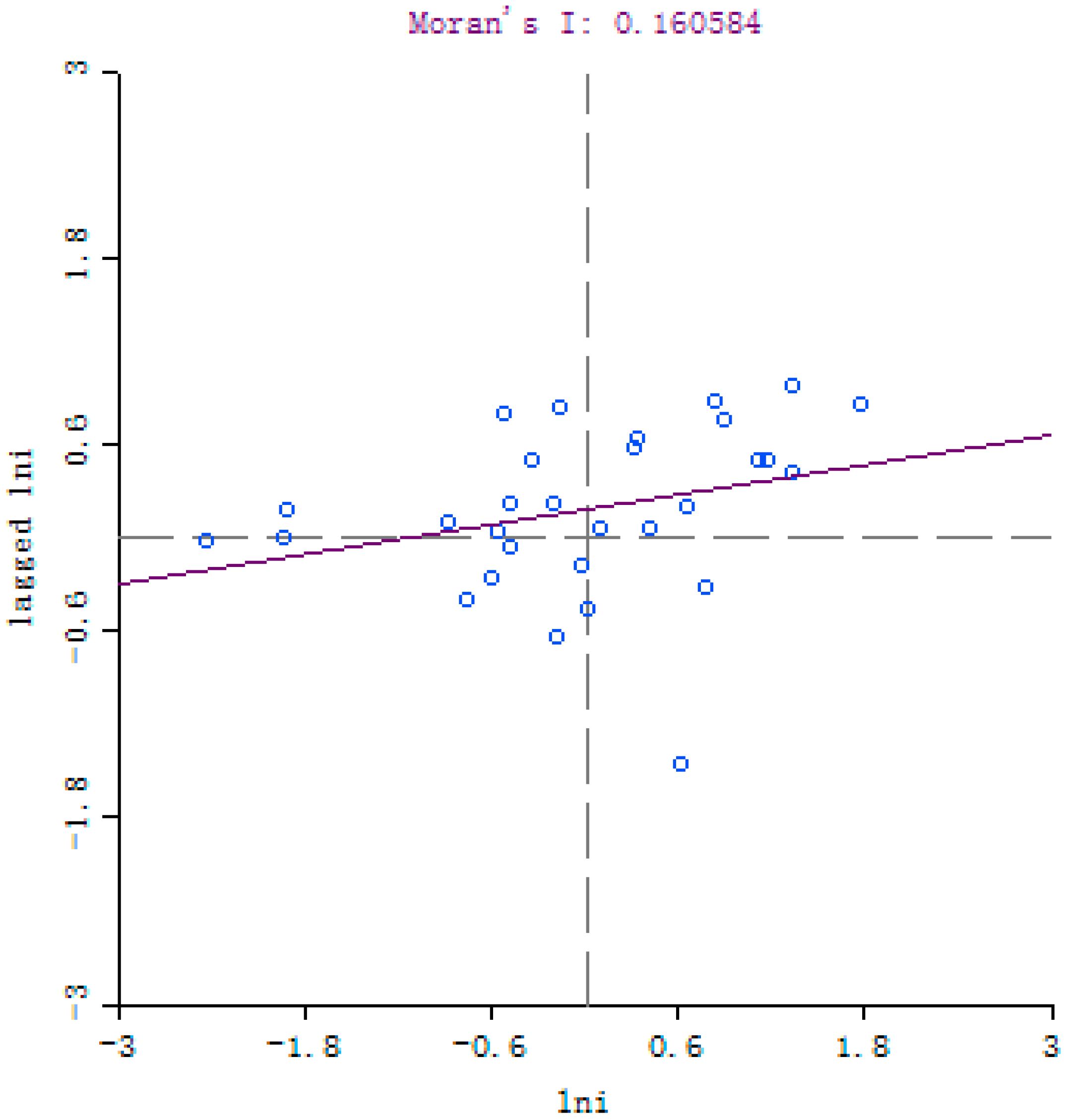
The Moran’s I index was used to test the spatial autocorrelation of regional carbon emissions in China, which can be seen in Figure 1.
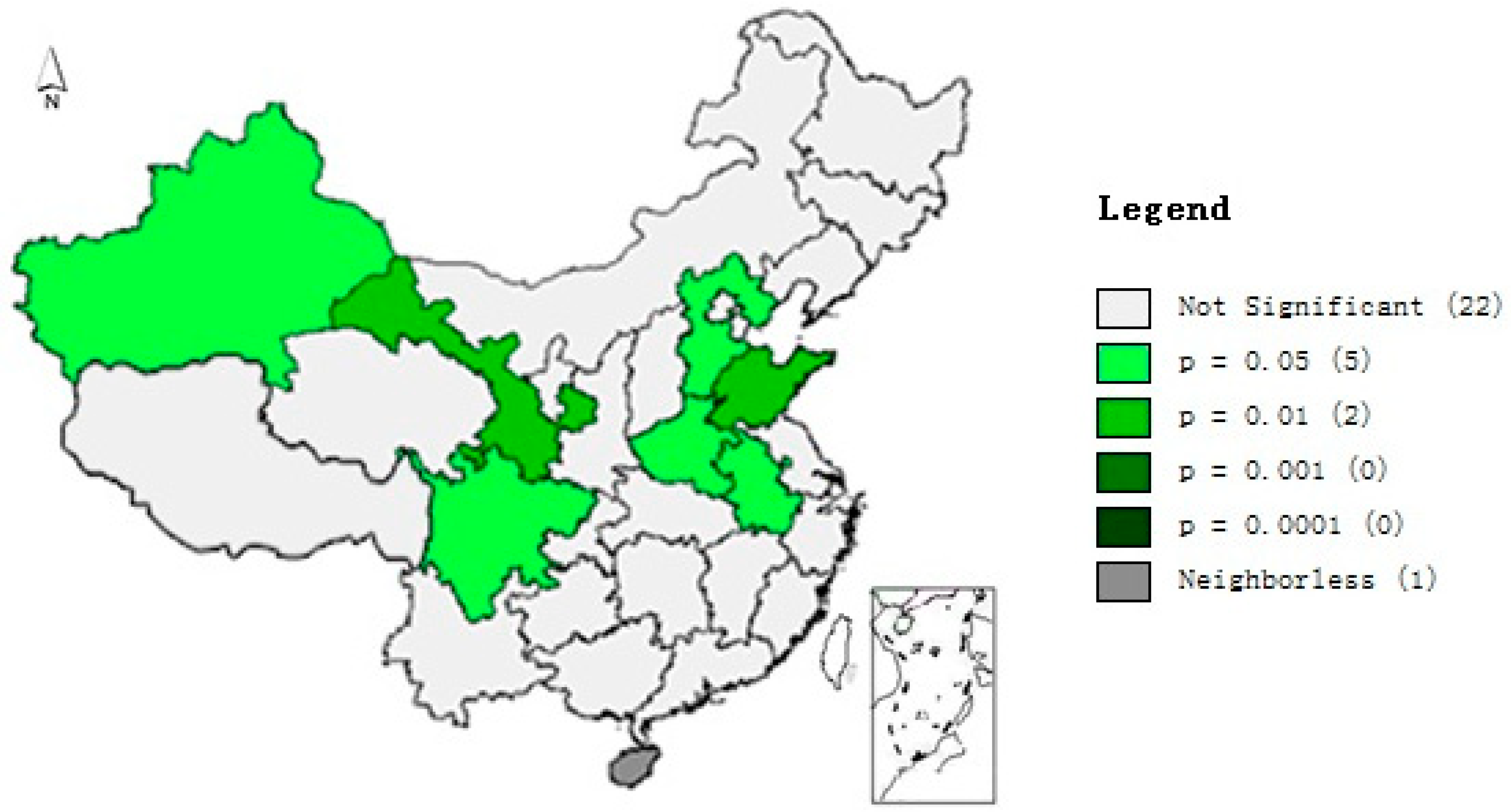
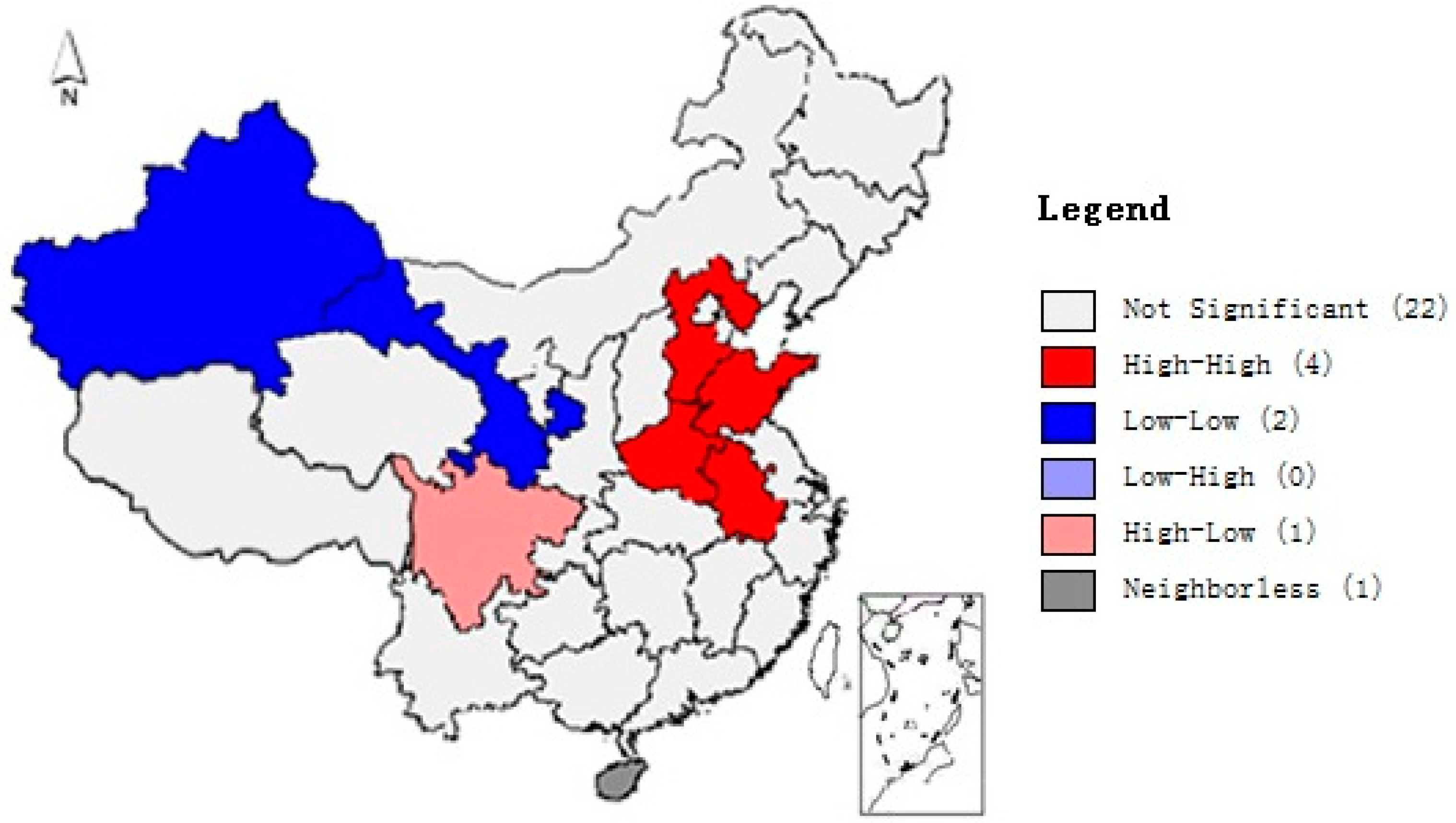
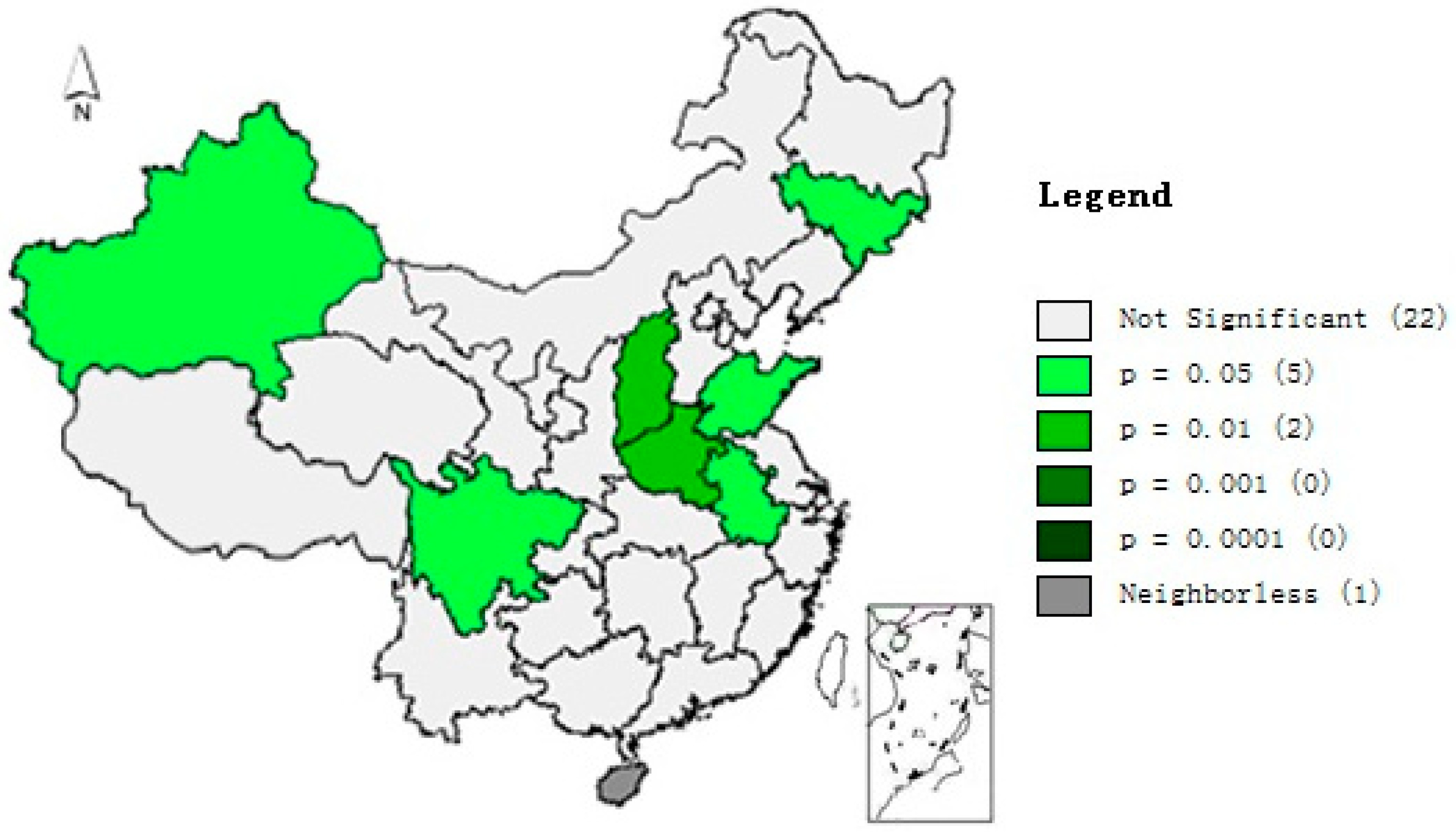
According to the mean carbon emission Moran scatter plots of 2000 and 2015 (Figure 1 and Figure 2), it can be seen that the mean concentration of carbon emissions in province is mostly concentrated in the first and third quadrants; the region of low carbon emissions is surrounded by other regions of low carbon emissions; and the region of high carbon emissions is surrounded by other regions of high carbon emissions, which proves that the carbon emissions in these provinces have the characteristics of agglomeration. Global spatial autocorrelation cannot be used to judge the spatial dependence of specific regions’ carbon emissions, so the local spatial correlation test is needed. The Moran scatter plot does not obtain the specific value of the local significance level of carbon emissions in the province. According to the regional agglomeration map and significance, it can more intuitively show the local spatial correlation and significance, and also provide evidence for the convergence of carbon emissions. Therefore, it is necessary to further calculate the local spatial autocorrelation statistical value. Moreover, the significance level indicates the need for provincial carbon emissions for the local spatial correlation index analysis (LISA). In order to distinguish the pattern of carbon emission clusters in local areas from 2000 to 2015, the focus of this study is to investigate the LISA index, and between 2000 and 2015, two periods were analyzed (As can be seen in the Figure 3, Figure 4, Figure 5 and Figure 6).
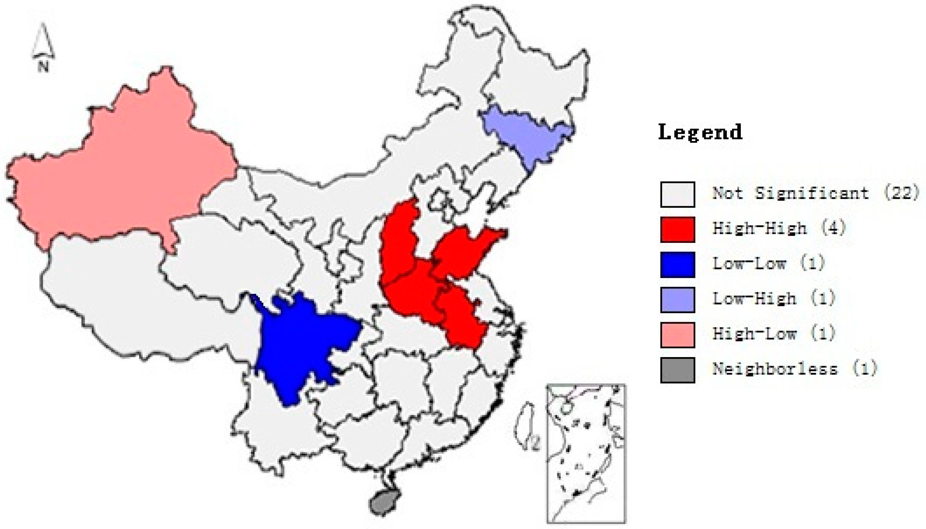
Local spatial autocorrelation LISA cluster maps are presented for the carbon emission levels of 30 provinces in China in 2000 and 2015. The red region indicates the provinces that have high carbon emission levels and are surrounded by other provinces with high carbon emission levels, and thus belong to the high carbon emission cluster region. The blue region indicates the provinces that have low carbon emission levels and which are surrounded by low carbon emission levels. The gray area indicates the provinces that have low carbon emission levels and which are surrounded by the provinces with high carbon emission levels. The pink area indicates provinces that have high carbon emission levels and which are surrounded by the provinces with low carbon emission levels. White areas represent regions with no significant spatial effect.
It can be seen that the carbon emissions of the Gansu and Shandong provinces in 2000 passed the 1% significance level test, and the carbon emissions of Xinjiang, Hebei, Henan, Anhui, and Sichuan provinces passed the 5% significance level test. Hainan Province is located in the L–H spatial outlier region, and Sichuan is located in the H–L spatial outlier region (L respective the low carbon emissions province; H respective the high carbon emissions province).
In 2015, the carbon emissions of Shanxi and Henan provinces passed the 1% significance level test, and five provinces, namely Jilin, Xinjiang, Shandong, Anhui, and Sichuan, passed the 5% significance level test. Jilin Province is located in the L–H-type spatial outlier area, and Xinjiang is located in the H–L-type regional spatial outlier area.
According to the LISA saliency map and the local LISA agglomeration map, it can be seen that China’s carbon emissions have formed a spatial agglomeration region in the regional spatial distribution of carbon emissions, which is a high-carbon-emission-level spatial cluster region, with Hebei Province at its center and including the surrounding provinces.

4.2. Empirical Analysis on the Econometric Model of the Spatial panel

First, the general panel model is used for regression. The Hausman test was used to determine whether to establish a random effect model or a fixed effect model, and then a general panel data model was established. According to the results of the study in Table 2, it can be seen that the Hausman test value of the panel data model is 38.0591. Through the significance test of 0.05%, the original hypothesis of establishing the random effect model is rejected. Therefore, the fixed effect model should be used.
Secondly, the effect of spatial spillover is tested. An ordinary least squares regression was carried out with MATLAB software, and LM-lag, LM-err, Robust LM-lag, and Robust LM-err tests were carried out simultaneously. According to the test results, as presented in Table 3, the spatial lag panel model and the spatial error panel model passed the 5% significance level test; the LM (Lagrangemultiplier) and Robust test values of the spatial lag panel model were 11.0838 and 6.5504, respectively; and the spatial error panel model’s LM and Robust test values were 10.496 and 6.3162, respectively, so the spatial lag panel should be adopted. The generalized least squares estimation method is used for the regression analysis of the panel data model in order to avoid the influence of heteroscedasticity.
The spatial panel model can be transformed into a spatial lag model and spatial error model, according to the Wald and LR (Likelihood Ratio) test. The test results show that the Wald_spatial_lag and LR_spatial_lag were 278.0052 and 243.4361, respectively; the adjoint probability values were 0; the Wald_spatial_error and LR_spatial_error were 187.3770 and 214.6246, respectively; and the adjoint probability was 0. This shows that the spatial lag panel model (SLPDM) is more wrong than the spatial lag panel model (SLPDM) concerning the increase of carbon emissions in the province, and the difference panel model (SEPDM) has a better effect.
Finally, the estimation results of three models were compared and analyzed by the ordinary panel data model, the spatial lag panel data model, and the spatial error panel data model. According to the previous results, the three models, namely the ordinary panel data model, the spatial lag panel data model, and the spatial error panel data model, should be estimated with the fixed effect model, and the data used in this study are processed logarithmically, which avoids the existence of the heteroscedasticity phenomenon. In this paper, the panel data model is selected to greatly increase the sample size, and at the same time, the sample’s degree of freedom is improved. The multiple collinearity of the explanatory variables, as well as the error, are also reduced. At the same time, the estimation results of the spatial lag panel data model and the spatial Dubin panel data model are compared and analyzed by the individual fixed effect, time fixed effect, and individual time double fixed effect.
Based on the panel data of 30 provinces in China from 2000 to 2015, the empirical results are shown in Table 4 and Table 5.
According to the Hausman test results, we should judge whether the standard panel data econometric model should adopt a fixed effect or random effect. The result of the Hausman test is 54.4961. The fixed effect model should be used to reject the original hypothesis that the individual effect and the explanatory variables are unrelated through the results of the significance tests. According to the model estimation and test results of Table 1, the R2 values of the fixed effect and the spatial fixed effect models are better than the random effect and the time random effect models. The Hausman test results of the spatial panel model and the standard panel model are the same, and the spatial panel fixed effect model of carbon emissions is a more reasonable model.
We can see that the logarithmic likelihood values of the spatial lag SLPDM model II and the SDPDM model VI are 200.667 and 264.3265, respectively, according to the model estimation, the test results of the spatial lag model, and the spatial Durbin model of China’s provincial domain carbon emissions, and the corresponding goodness of fit coefficients are 0.8585 and 0, respectively. The value of 0.8841 is relatively high, and according to the actual situation of this country, the economic meaning of the model is obvious. Therefore, this paper chooses the SLPDM model II and SDDM model VI to carry out empirical research on the elasticity coefficient and spatial spillover effect of various factors affecting carbon emissions in China.
The estimation results of the spatial fixed effect SLPDM model II in Table 5 show that economic growth, industrial structure, financial development, and the elasticity coefficient of the urbanization rate are positive, and they all have positive effects on the growth of carbon emissions through a significance test. Without considering other factors, an economic growth of 1% can lead to a 0.8217% increase in the growth of carbon emissions in our province and 1% of growth in the industrial structure, which leads to a 0.6255% increase in the growth of China’s provincial carbon emissions, a 0.1279% increase in the growth of China’s provincial carbon emissions, and a 1% increase in the financial development index and the rate of urbanization per year. The increase of 1% has led to a 0.2865% increase in the growth of China’s provincial carbon emissions. Population, technological progress, and energy prices have a negative effect on carbon emissions. Population and technological progress have passed the significance level test. The effect of energy price and export dependence on carbon emissions is not significant, and it may reduce the high energy consumption and high emissions in China. The export trade has been adjusted to a significant effect, and it is also consistent with the development stage of China’s market economy.
The spatial fixed effect model in Table 5 shows that the economic growth, industrial structure, financial development, and the elasticity coefficient of urbanization rate are positive; that is, they have a positive effect on the growth of carbon emissions. Under the conditions of other factors, economic growth is 1%, which can lead to the increase of carbon emissions in the provinces of China by 1.3106%. The growth of 1% of the industrial structure leads to a 0.3215% increase in the growth of China’s provincial carbon emissions and an increase of 1% in the financial development index, which can lead to a 0.1216% increase in the growth of China’s provincial carbon emissions and a 1% increase in the urbanization rate, resulting in a 0.1658% increase in the growth of China’s provincial carbon emissions, the population, technological progress, and energy prices relating to carbon emissions. Negative effects, energy prices, and export dependence are opposed, but population, technological progress, energy prices, and export dependence have not passed the significance test on China’s provincial carbon emissions. Therefore, according to the impact of the carbon emissions on the elastic coefficient, we can see that the carbon emissions from the current economic development and other factors need to be solved, and the technological progress in reducing the carbon emission capacity needs to be strengthened.
The regression results shown in Table 5 also indicate that the ρ valueof the SDPDM model VI (0.3110) of the spatial fixed effect passes the significance level test of 0.1%. It can be seen that the carbon emissions from the neighboring provinces increase by 1% and the provincial carbon emissions increase by 0.311%, in the case of considering, and not considering, respectively, the adjacent lag effect of the explanatory variable space. It can be seen that in the analysis of regional carbon emissions’ growth, the traditional panel data model, which does not consider the spatial effect, is biased. There are obvious spatial spillovers in the influencing factors affecting carbon emissions in the neighboring provinces and the growth of carbon emissions. It is proved that there is interaction between the explanatory variables in the provincial carbon emission model and between the explanatory variables. In the process of China’s provincial carbon emissions growth, the influence factors affecting the different carbon emissions in a provincial region can lead to an increase or decline of carbon emissions in the neighboring provinces. The influencing factors in the provinces and the adjacent provincial factors have little difference, which drives the change in carbon emissions in the provincial regions of China. This kind of spatial spillover effect on China’s low carbon emissions, and the transition to a low-carbon economy in the regions, is of great significance.

5. Conclusions and Policy Recommendation

China’s provincial carbon emissions have obvious spatial dependence and obvious spatial agglomeration. In this paper, the spatial panel data model is established for the first time, and the contribution of different factors to carbon emissions’ growth is accurately estimated. The influencing factors and the spatial spillover effects affecting carbon emissions’ growth are examined. The spatial lag and spatial error model of this paper show the following points: (1) There is a significant spatial correlation in the growth of carbon emissions of the provinces, and the industrial cluster phenomenon is obvious in all the provinces. Therefore, the correlation in the process of carbon emissions’ growth must be fully considered in the study of carbon emissions’ growth in China. (2) Economic growth, industrial structure, financial development, and the elastic coefficient of the urbanization rate are positive; that is, they have a positive effect on carbon emissions’ growth. Under the conditions of other factors, economic growth and industrial structure are the main factors that lead to carbon emissions’ growth. Among the factors affecting survival and fiscal decentralization, China is an aging country with a large income gap. The development stage leads to the opposite effect to the increase in population size on carbon emissions, and the role of technological progress and other factors that reduce carbon emissions need to be improved. (3) The influencing factors affecting the carbon emissions in the neighboring provinces and the growth of carbon emissions have a spatial spillover effect. In the process of carbon emissions’ growth in China, the industrial structure will have a significant role in promoting the growth of carbon emissions in the surrounding provinces.
According to the results of the empirical study and the actual situation in China, our suggestions in relation to policy changes concerning the reduction of the growth of the provincial carbon emissions are as follows: (1) It can be seen that China’s carbon emissions have an overall linkage mechanism, and the development characteristics of different regions are different, leading to different factors affecting carbon emissions. Moreover, regional carbon emissions have spatial dependence, a cluster effect, and path dependence, and carbon emissions and different factors have a spatial spillover effect and adjacent regional carbon emissions. Emissions and their influencing factors have spatial spillover effects, so we can design the theory and path of regional carbon emission joint prevention and control according to the linkage mechanism of spatial carbon emissions. (2) The growth of carbon emissions in the provincial regions of China is spatially dependent, which means that the government must consider the locationality of carbon emissions’ growth when making carbon emission policies and related indicators. In considering the spillover effect, it is crucial to pay full attention to the cooperation and exchange of low-carbon technology in adjacent areas, in order to accelerate the cross-regional governance of carbon emissions and restrain the effect of industrial structure on the growth of carbon emissions in adjacent areas. (3) It is crucial to take corresponding measures into account to form the interaction mechanism of the influencing factors affecting provincial carbon emissions, optimize the spatial efficiency of interprovincial factors, reduce the synergistic contribution rate of influencing factors affecting carbon emissions’ growth, and increase the contribution rate of influencing factors affecting carbon emissions’ growth. (4) Controlling carbon emissions has become an urgent problem with the continuous deepening of China’s economic development, changing the mode of economic growth and adjusting the industrial structure. In connection with financial reform and export trade, the important premise of low-carbon economic development should be considered. Low-carbon technology is an important way to achieve carbon emissions’ reduction and accelerate green finance. In the transition of international trade, the government and other relevant departments should take into account the different influencing factors as well as the difference in carbon emissions by the different influencing factors and the spatial action mechanism.

Author Contributions

X.T. designed the analytical framework, and wrote and revised the paper. X.L. co-wrote and revised the paper, L.T. constructed the model and analyzed the data. X.J. assisted the collcetiong of research data. All authors read and approved the final manuscript.

Funding

The work was supported by the fund of China Scholarship Council; the China Postdoctoral Science Foundation, Project approval number: 2016M601240; the Liaoning Social Sciences Joint Economic and social development research topics, Project approval number: 20191slktyb-005; and the 2018 Qinhuangdao social sciences development research topic, Project approval number: 201807104.

Acknowledgments

We are enormously grateful to reviewers and editors for the time they have spent on studying the manuscript and their valuable comments on improving it.

Conflicts of Interest

The authors declare no conflict of interest.

References

  1. Christidou, M.; Panagiotidis, T.; Sharma, A. On the stationarity of per capita carbon dioxide emissions over a century. Econ. Model. 2013, 33, 918–925. [Google Scholar] [CrossRef] [Green Version]
  2. Dergiades, T.; Kaufmann, R.; Panagiotidis, T. Long-run changes in radiative forcing and surface temperature: The effect of human activity over the last five centuries. J. Environ. Econ. Manag. 2016, 76, 67–85. [Google Scholar] [CrossRef]
  3. Wu, L.; Kaneko, S.; Matsuoka, S. Driving Forces behind the Stagnancy of China’s Energy-related CO2 Emissions From 1996 to 1999: The Relative Importance of Structural Change, Intensity Change and Scale Change. Energy Policy 2005, 33, 319–335. [Google Scholar] [CrossRef]
  4. Zhao, Q.; Yan, Q.; Zhao, H. Research on Spatial Characteristics and Influencing Factors of Provincial Carbon Emissions in China. J. Beijing Inst. Technol. (Soc. Sci. Ed.) 2018, 20, 9–16. [Google Scholar]
  5. Li, J.; Chen, Y.; Li, Z.; Liu, Z. Quantitative Analysis of the Impact Factors of Conventional Energy Carbon Emissions in Kazakhstan Based on LMDI Decomposition and STIRPAT Model. Univ. Chin. Acad. Sci. J. Geogr. Sci. 2018, 28, 1001–1019. [Google Scholar] [CrossRef]
  6. Li, N.; Shi, M.; Yuan, Y. Impacts of Carbon Tax Policy on Regional Development in China: A Dynamic Simulation Based on a Multi-regional CGE Model. Acta Geogr. Sin. 2010, 65, 1569–1580. [Google Scholar]
  7. Weber, C.L.; Peters, G.P.; Guan, D. The contribution of Chinese exports to climate change. Energy Policy 2008, 36, 3572–3577. [Google Scholar] [CrossRef] [Green Version]
  8. Wang, C.; Chen, J.; Zou, J. Decomposition of energy-related CO2 emission in China: 1957–2000. Energy 2005, 30, 73–83. [Google Scholar] [CrossRef]
  9. Wang, H.; He, C. Energy Consumption, Economic Growth and CO2 Emissions in China: Analysis Based on Logarithm Mean Divisa Decomposure Method. Resour. Environ. Yangtze Basin 2010, 19, 18–23. [Google Scholar]
  10. Dhakal, S.; Shinji, K.; Hidefumi, I. CO2 Emissions from energy use in East Asian mega-cities: Driving factors and their contributions. Environ. Syst. Res. 2003, 31, 209–216. [Google Scholar] [CrossRef]
  11. Li, L.; Liu, J. Using LMDI to Analyze the Driving Forces in Industrial CO2 Intensity: Evidence for Xinjiang. Ecol. Econ. 2011, 4, 34–38. [Google Scholar]
  12. Zhao, A.; Li, D. EKC Test for China’s Carbon Dioxide Emissions and Analysis of Affecting Factors. Sci. Sci. Manag. S & T 2012, 33, 107–115. [Google Scholar]
  13. Fan, T.; Luo, R.; Fan, Y.; Zhang, L.; Chang, X. Study on Influence Factors for carbon Dioxide Emissions in China’s Chemical Industry with LMDI Method. China Soft Sci. 2013, 3, 166–174. [Google Scholar]
  14. Zhang, L.; Lei, J.; Zhang, X. Variation and Influent Factor of Carbon Emission of Primary Energy Consumption in Xinjiang during the Period 1952–2008. Resour. Sci. 2012, 34, 42–49. [Google Scholar]
  15. Song, D.; Lu, Z. The Factor Decomposition and Periodic Fluctuations of Carbon Emission in China. China Popul. Resour. Environ. 2009, 19, 18–24. [Google Scholar]
  16. He, W.; Zhang, K. The Decomposition on the Influencing Factors of China’s Steel Industry Carbon Emission. J. Ind. Technol. Econ. 2013, 1, 3–10. [Google Scholar]
  17. Zhu, Q.; Peng, X.Z.; Lu, Z.M.; Wu, K.Y. Factors Decomposition and Empirical Analysis of Variations in Energy Carbon Emission in China. Resour. Sci. 2009, 31, 2072–2079. [Google Scholar]
  18. Li, G.; Li, Z. Regional Difference and Influence Factors of China’s Carbon Dioxide Emissions. China Popul. Resour. Environ. 2010, 20, 22–27. [Google Scholar]
  19. He, X.; Zhang, Y. Influence Factors and Environmental Kuznets Curve Relink Effect of Chinese Industry’s Carbon Dioxide Emission—Empirical Research Based on STIRPAT Model with Industrial Dynamic Panel Data. China Ind. Econ. 2012, 1, 26–35. [Google Scholar]
  20. Zhu, Q.; Peng, X.Z.; Lu, Z.M.; Yu, J. Analysis Model and Empirical Study of Impacts from Population and Consumption on Carbon Emissions. China Popul. Resour. Environ. 2010, 20, 98–102. [Google Scholar]
  21. Qiang, H.E.; Guangming, L.V. Analysis of Ecological Environmental Impact Based on IPAT Model: A Case Study of Beijng. J. Central Univ. Finance Econ. 2008, 12, 83–88. [Google Scholar]
  22. Zhu, Y.; Zhang, S. Analysis of driving factors of Beijing’s economic carbon emissions based on STIRPAT model. Spec. Zone Econ. 2012, 1, 77–79. [Google Scholar]
  23. Tong, X.; Chen, K.; Li, G. Influencing Factors Analysis and Trend Forecasting of China’s Carbon Emissions: Empirical Study Based on STIRPAT and GM(1, 1) Models. J. Northeast Univ. (Nat. Sci.) 2015, 36, 297–300. [Google Scholar]
  24. York, R.; Rosa, E.A.; Dietz, T. STIRPAT, IPAT and impacts: Analytic tools for unpacking the driving forces of environmental impacts. Ecol. Econ. 2003, 46, 351–365. [Google Scholar] [CrossRef]
  25. Xu, G.; Liu, Z.; Jiang, Z. Decomposition Model and Empirical Study of Carbon Emissions for China, 1995–2004. China Popul. Resour. Environ. 2006, 16, 158–161. [Google Scholar]
  26. Hu, C.; Huang, X.; Zhong, T. Character of Carbon Emission in China and Its Dynamic Development Analysis. China Popul. Resour. Environ. 2008, 18, 46–50. [Google Scholar]
  27. Wu, Y. Spatial Panel Econometric of Tourism Economic Growth and Spillover Effects. Tour. Trib. 2014, 29, 16–24. [Google Scholar]
  28. IPCC. 2006 IPCC Guidelines for National Greenhouse Gas Inventories; IGES: Hayama, Japan, 2016. [Google Scholar]
  29. Wang, K.; Wang, C.; Chen, J. Analysis of the economic impact of different Chinese climate policy options based on a CGE model incorporating endogenous technological change. Energy Policy 2009, 37, 2930–2940. [Google Scholar] [CrossRef]
  30. Birdsall, N. Another Look at Population and Global Warming: Population, Health and Nutrition Policy Research; Working Paper; World Bank: Washington, DC, USA, 1992. [Google Scholar]
  31. Knapp, T.; Mookerjee, R. Population Growth and Global CO2 Emissions. Energy Policy 1996, 24, 31–37. [Google Scholar] [CrossRef]
  32. Tan, D.; Huang, X.; Hu, C. Analysis of the Relationship between Industrial Upgrading and Carbon Emission in China. Sichuang Environ. 2008, 2, 74–84. [Google Scholar]
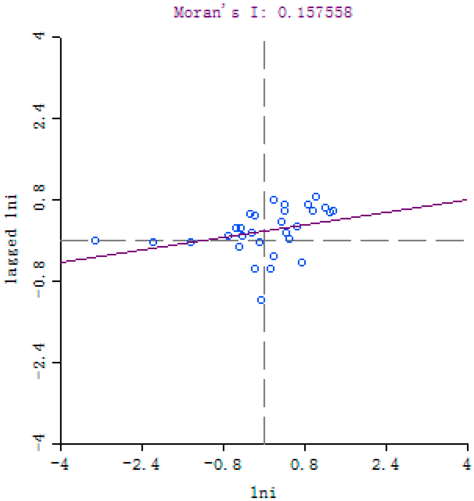
Figure 1. Moran scatter plot showing the mean value of carbon emissions in 2000. (i respective the carbon emissions).
Sustainability 10 04739 g001
Figure 2. Moran scatter plot showing the mean value of carbon emissions in 2015.
Sustainability 10 04739 g002
Figure 3. Local indicators of spatial association (LISA) significance map based on the first-order matrix of carbon emissions in 2000. Numbers in brackets represent the number of regions in that category.
Sustainability 10 04739 g003
Figure 4. LISA cluster map based on the first-order matrix of carbon emissions in 2000.
Sustainability 10 04739 g004
Figure 5. LISA significance map based on the first-order matrix of carbon emissions in 2015.
Sustainability 10 04739 g005
Figure 6. LISA cluster map based on the first-order matrix of carbon emissions in 2015.
Sustainability 10 04739 g006
Table 1. Standard coal (SC) coefficients of carbon emissions of different energy sources (in kg C * or kg SC).
Data ResourceCoalOilNatural Gas
US Department of Energy/Energy Information Administration0.7020.4780.389
Japan Institute of Energy Economics0.7560.5860.449
Chinese Academy of Engineering0.680.540.41
National Greenhouse Gas Control Project0.7480.5830.444
National Science and Technology Commission Climate Change Project0.7260.5830.409
Beijing Project of the State Science and Technology Commission0.6560.5910.452
Energy Research Institute of National Development and Reform Commission0.74760.58250.4435
* C: Carbon emissions.
Table 2. Hausman estimates of the ordinary panel model.
Test SummaryChi-Sq. StatisticChi-Sq. d.f. *Prob.
Random cross-section38.059190.0000
* Regression is significant at the 0.05.
Table 3. Spatial correlation of the model test.
Spatial Correlation TestTest MethodStatistical Valuep-Value
LM test, no spatial lag *11.08380.001
Robust LM test, no spatial lag6.55040.010
LM test, no spatial error10.84960.001
Robust LM, test no spatial error6.31620.012
* LM (Lagrangemultiplier) regression is significant at the 0.05.
Table 4. Results of the standard panel econometric models for carbon emissions in the provinces.
VariableNo Fixed EffectsFixed EffectsRandom EffectsSpatial Fixed EffectsTime Period Fixed Effects
C−0.8526−1.5471−0.8526−1.1804−0.9880
LnP0.01870.28850.01870.25450.0257
LnA0.93820.61980.93820.67070.9305
LnT−0.2736−0.2570−0.2736−0.2607−0.2723
LnS1.63511.56271.63511.53291.6497
LnF0.15560.62220.15560.08120.1538
LnE−0.5451−0.4269−0.5451−0.4669−0.5390
LnEX−0.1003−0.0301−0.1003−0.0320−0.1028
LnU−0.11080.0615−0.11080.0120−0.0958
LnFD0.17620.24720.17630.23250.1755
R20.78500.80950.78510.80810.7858
P respective Population; A respective Economic growth; T respective Technological progress; S respective Industrial structure; F respective Financial development; E respective Energy price; EX respective International Trade; U respective The rate of urbanization; FD respective Fiscal decentralization.
Table 5. Spatial econometric models for estimating carbon emissions in the provinces.
VariableSLPDM 1SDPDM 2
No Fixed Effects ISpatial Fixed Effects IITime Period Fixed Effects IIISpatial and Time Period Fixed Effects IVNo Fixed Effects VSpatial Fixed Effects VITime Period Fixed Effects VIISpatial and Time Period Fixed Effects VIII
C0.1689 −3.3062
LnP−0.0045−0.41030.1810−0.69110.1852−0.09880.2372−0.5147
LnA0.99070.82170.72310.28380.78911.31060.68110.7550
LnT−0.2965−0.1532−0.3315−0.1152−0.2388−0.0515−0.2497−0.0200
LnS1.33990.62551.26240.68961.12900.32151.11730.4339
LnF0.13220.12790.05170.12550.13550.12160.10680.0967
LnE−0.56480.1918−1.4017−0.28160.24710.0332−0.8388−0.1871
LnEX−0.0664−0.01930.0195−0.07460.10110.03500.1431−0.0409
LnU−0.21130.2865−0.06260.2030−0.24350.1658−0.21770.0249
LnFD0.11230.04690.26200.06980.0723−0.01700.12890.0088
WlnP −0.0827−0.87260.2136−0.8286
WlnA −0.1761−0.7375−0.2833−1.0520
WlnT −0.0245−0.0527−0.18460.1048
WLnS 0.95310.37751.13610.6726
WLnF −0.02960.03590.01000.0772
WLnE −1.0680.1016−1.5495−0.3011
WLnEX −0.2853−0.1138−0.1843−0.2753
WLnU 0.5109−0.17590.8132−0.1093
WLnFD 0.02190.12050.07750.0566
ρ0.0600−0.03000.06400.26250.33900.31100.34000.0330
logL−254.3434200.0667−255.7443207.1831−167.7281264.3265−712.9441328.9011
R20.79040.96850.79760.97300.85770.97640.86510.9815
Adj. R20.78740.85850.74160.29710.83790.88410.42470.5618
1 SEPDM: Spatial Error Panel Data Model; 2 SDPDM: Spatial Durbin Panel Data Model.