Evaluating Impacts of Overloaded Heavy Vehicles on Freeway Traffic Condition by a Novel Multi-Class Traffic Flow Model

Abstract

Overloaded heavy vehicles (HVs) have significant negative impacts on traffic conditions due to their inferior driving performance. Highway authorities need to understand the impact of overloaded HVs to assess traffic conditions and set management strategies. We propose a multi-class traffic flow model based on Smulders fundamental diagram to analyze the influence of overloaded HVs on traffic conditions. The relationship between the overloading ratio and maximum speed is established by freeway toll collection data for different types of HVs. Dynamic passenger car equivalent factors are introduced to represent the various impacts of overloaded HVs in different traffic flow patterns. The model is solved analytically and discussed in detail in the appendices. The model validation results show that the proposed model can represent traffic conditions more accurately with consideration for overloaded HVs. The scenario tests indicate that the increase of overloaded HVs leads to both a higher congestion level and longer duration.

1. Introduction

Heavy vehicles (HVs) have significant impacts on traffic conditions. However, it is a common practice in China for commercial carriers to overload (i.e., load trucks with goods heavier than the factory recommended weight limit) their fleets to reduce their operating costs [1]. Compared with conforming HVs, overloaded ones suffer from lower speeds, inferior acceleration and deceleration performances, and, consequently, impose more significant impacts on traffic conditions.

Unfortunately, overloaded HVs are frequently observed on freeways in most parts of China and many developing countries, such as India, Thailand, Vietnam, etc. In China, if one heavy vehicle is detected as an overloaded heavy vehicle, the toll station staffs will still allow this heavy vehicle entering the freeway but charge additional fines for overloading. This is because there is not enough space to unload and temporarily store the overloaded goods in the toll station plaza, and the long stop at the toll station will obstruct the subsequent vehicles entering the freeway. Therefore, the toll station staff will not forbid the overloaded HVs entering the freeway, but punish with fines, which mainly considers the pavement fatigue, but not the negative impacts on traffic condition. However, the profit from overloading can cover the additional cost and, therefore, many heavy vehicles choose to overload. For example, the average overloading proportion (i.e., the total number of overloaded HVs/population of HVs) on the freeway is 15%, and it could be more than 40% at midnight in eastern China. Furthermore, the average overloading ratio (i.e., (total weight − weight limit)/weight limit) is 35%, and the overloading ratio of tractor-trailers could exceed 100% in some extreme circumstances [2,3]. The average reduction of overloaded HVs’ travel speeds is 16% compared with HVs with the same configuration but loaded at capacity [4].

The problems induced by overloaded HVs are significant, and there are a number of studies that focus on the impacts on pavement fatigue life and distress, while the impacts of overloaded HVs on freeway traffic conditions have not been properly analyzed to the best of our knowledge. The effect of HVs is captured by the Passenger Car Equivalent (PCE) factor in the Highway Capacity Manual (HCM 2010) [5]. However, the different effects of overloaded and normal HVs are not distinguished. Moreover, the impacts of HVs vary from different traffic conditions [6], while the fixed PCE factors in the HCM are sensitive neither to the presence of overloaded HVs nor to various traffic conditions. This research aims to quantitatively evaluate the traffic impact of overloaded HVs on traffic conditions, and this will contribute to refine the management strategies of freeway overloaded HVs and guarantee the sustainable development of freeway transportation.

We developed a multi-class traffic flow model to analyze the impact of overloaded HVs on traffic conditions. The model can be used to estimate traffic conditions in real-time and evaluate traffic management strategies with consideration for the presence of overloaded HVs. First, the relationship between vehicle weight and driving performance is established to distinguish the diverse driving performances between overloaded HVs and normal ones. Next, a dynamic PCE is introduced to represent the diverse impacts of overloaded HVs under different traffic conditions. Then, the formulation of effective density and effective volume is proposed. After that, an empirical study is conducted to evaluate the accuracy of the proposed model. Finally, several scenario tests are performed to verify the model results and to represent the sensitivity of overloaded HVs with different overloading proportions.

The paper is organized as follows: Section 2 summarizes the previous research in multi-class traffic flow models and the development of dynamic PCE. Section 3 describes the freeway toll data used in this study and the relationship between the overloading ratio and maximum speed. Section 4 discusses the process to establish the multi-class kinematic wave traffic flow model. Section 5 presents an empirical study to validate model results with real traffic data. Section 6 presents several scenario tests to show the impacts of overloaded HVs in different traffic demand and supply combinations. Finally, Section 7 concludes the study with a discussion of the study results and suggestions for future research.

2. Literature Review

Overloaded HVs, characterized by their inferior driving performance (such as lower running speed and larger minimum safe headway), tend to impose negative impacts on traffic conditions under different traffic flow patterns. However, the impact of overloaded HVs has not been carefully addressed in previous multi-class macroscopic traffic flow models.

The presence of HVs causes larger space and time headways and longer reaction time [7]. Vehicle weight is one of the critical factors that determine running, braking, and handling performance [8]. For example, the minimum safe headway of HVs depends on reaction time and stopping distances, which, in turn, depend on the total vehicle weight. Therefore, overloaded HVs need larger headways than normal ones. Meanwhile, the desired travel speed is not only limited by traffic conditions but also constrained by the vehicle’s own weight [9]. The desired travel speed decreases with increased vehicle weight in the free flow condition. Thus, overloaded HVs need to be considered separately when analyzing their impacts on traffic conditions due to distinguishable driving performance.

PCE describes the relative impact of a vehicle on traffic conditions when compared with a typical passenger car. In the development of PCE, the equivalency criterion varies from flow rates and density, headways, queue discharge flow, speed, delays, v/c ratio, etc. [10,11]. The PCE value of each vehicle type is typically constant. However, the impact of HVs varies under different traffic conditions [12]. It is noticed that the impact of HVs under congestion is greater than under the free-flow condition [13]. The cycle of acceleration-deceleration is more recurrent under congestion since the acceleration and deceleration performances of HVs are inferior. Moreover, it is also mentioned that PCE depends on the presence of HVs [5,14]. When there are more HVs on a freeway, the HVs could form platoons and have less interaction with passenger cars. Thus, the PCE of each HV in platoons should be smaller than individual HVs, although the total impacts from HVs increase with the amount of HVs. In conclusion, the previous studies suggest that the PCE of HVs should vary with traffic conditions and the proportion of HVs. Mehar (2013) [15] suggested PCU values for different types of vehicles at different levels of service and for different traffic compositions. Van Lint (2008) [16] proposed a continuous dynamic PCE based on space occupancy. The dynamic PCE value depends on speed, time headway, and vehicle length of both HVs and passenger cars. However, the dynamic PCE is not sensitive to the proportion of HVs, and the more severe impact of overloaded HVs on traffic conditions is not considered in this PCE formulation.

Recently, multi-class traffic flow models have been discussed frequently in order to describe non-linear traffic phenomena, which cannot be reproduced by aggregate class models [17,18]. In order to identify driving characteristics among different vehicle types and simultaneously reduce computational burdens for online traffic control, multi-class kinematic wave traffic flow models are proposed [19,20]. In multi-class kinematic wave traffic flow models, vehicle types are distinguished by driving performance and vehicle physical properties, such as speed and vehicle length. Daganzo (2002) [21] proposed a multi-class model for two vehicle types (i.e., passenger car and HV) according to travel speed. Chanut and Buisson (2003) [22] pointed out that vehicles are differentiated not only by their speeds but also by their lengths, and they established a two-flow traffic model. Ngoduy and Liu (2007) [23] formulated a multi-class first-order traffic flow model for the faster car, slower car, and HV vehicle types, where each type is characterized by their desired speeds in free-flow and all vehicles are traveling at the same speed under congestion. Van Wageningen-Kessels (2013, 2014) [24,25] developed a multi-class continuum traffic flow model that accounts for the differences between vehicle types, such as maximum speed, headway, and vehicle length.

Although travel speed has been consistently identified as a critical factor for vehicle type identification, overloaded HVs have never been classified as a standalone vehicle type in previous literature. The contributions of this study include the following.

(1)

A new dynamic PCE was designed for overloaded HVs, and it can represent the different influences present when traffic conditions change.

(2)

A new multi-class kinematic wave traffic flow model based on dynamic PCE is proposed with consideration for the driving performances of overloaded HVs.

(3)

The impacts of overloaded HVs on freeway traffic conditions are analyzed based on scenario tests.

3. Data and Vehicle Type Description

3.1. Freeway Toll Data

Each vehicle enters and exits the freeway by toll station in China, and the freeway toll data contains the trip information of each vehicle traveling on a freeway, such as the entry/exit time, entry/exit station, total weight, and vehicle type (i.e., the weight-limit can be known for each heavy vehicle). The toll fee for heavy vehicles is based on the vehicle type, travel distance, and total weight. In this case, each entrance ramp of toll station is equipped with a wagon balance to obtain the weight information of each vehicle. Therefore, it is easy to confirm whether one heavy vehicle is overloaded or not, and the overloading proportion and ratio can be calculated accurately by the freeway toll data. The traffic conditions, including traffic demand and travel time, can be estimated using freeway toll data with proper data quality control [26]. The real travel time, which will be used to acquire free-flow travel speeds for model calibration and validation in each time interval, can be calculated using Equation (1):

$$T_{(i,j)}^k=\frac{{\displaystyle \sum _{n=1}^{N_{(i,j)}^k}(t_{en(n)}^k-t_{ex(n)}^k)}}{n_{(i,j)}^k}-(t_{on(i)}^k+t_{off(j)}^k)$$

(1)

where $T_{(i,j)}^k$ is the travel time from entry station i to exit station j during time period k, $N_{(i,j)}^k$ is the sample size from toll station i to j after data quality control during time period k, $t_{en(n)}^k$ is the entry time of vehicle n entering during time period k, $t_{ex(n)}^k$ is the exit time of vehicle n, and $t_{on(i)}^k$ and $t_{off(j)}^k$ are the travel time on the on-ramp of entry station i and the off-ramp of exit station j, respectively, which can be calculated using the loop detector data on the ramp.

3.2. Characteristics of Different Vehicle Types

Freeway toll data records the vehicle type of passenger cars (i.e., PC1, PC2, …, PC4) and heavy vehicles (i.e., HV1, HV2, …, HV5) separately. PCs are classified by vehicle capacity while HVs are classified by total weight limit. Based on the vehicle type information, the volume proportion of PC1 can be calculated. Additionally, the travel speed of each vehicle can be calculated by entry/exit time and the distance between the entry/exit stations. The freeway toll data of the whole Jiangsu freeway network during July 2012 were utilized, and the characteristics of each classification are shown in

Table 1. Characteristics of different passenger cars and heavy vehicles.

Type ID	Classification Criteria PC: Vehicle Capacity HV: Total Weight Limit	Vehicle Length (m)	Traffic Volume Proportion in Jiangsu Province (%)	90% Percentile Highest Travel Speed (km/h)
PC1	≤7 seats	3.5–6	68.6	117.5
PC2	8–9 seats	6–9	2.0	100.9
PC3	20–29 seats	9–12	0.9	95.4
PC4	≥40 seats	12–13.7	1.3	93.8
HV1	≤2 t	3.5–4.5	6.2	90.6
HV2	2–5 t (inclusive of 5 t)	4.5–6	9.1	87.2
HV3	5–10 t (inclusive of 10 t)	6–8	4.1	84.1
HV4	10–15 t (inclusive of 15 t)	8–12	4.5	82.0
HV5	>15 t	12–16.5	3.3	79.0

. In most cases, small passenger cars (i.e., PC1, the type 1 passenger car) comprise the largest proportion of traffic volume on the freeway. For example, the freeway volume proportion of PC1 in Jiangsu province is 68.6% (Table 1), while the subtotal of PC2 (i.e., the type 2 passenger car), PC3, and PC4 altogether is merely 4.3%. Since PC2, PC3, and PC4 only comprise a small proportion of the vehicle population, these volumes are omitted in the modeling process for simplification. In this study, only PC1, HV1 (i.e., the type 1 heavy vehicle), HV2, HV3, HV4, and HV5 are modeled.

Due to their different mechanical performances, each vehicle type has a specific maximum speed in the free flow condition. Taking the 90th percentile of the highest travel speed as the maximum speed of each vehicle type (non-overloaded vehicles) in free-flow, the results are shown in Table 1. The largest speed gap existing between PC1 and HV5 is 38.5 km/h.

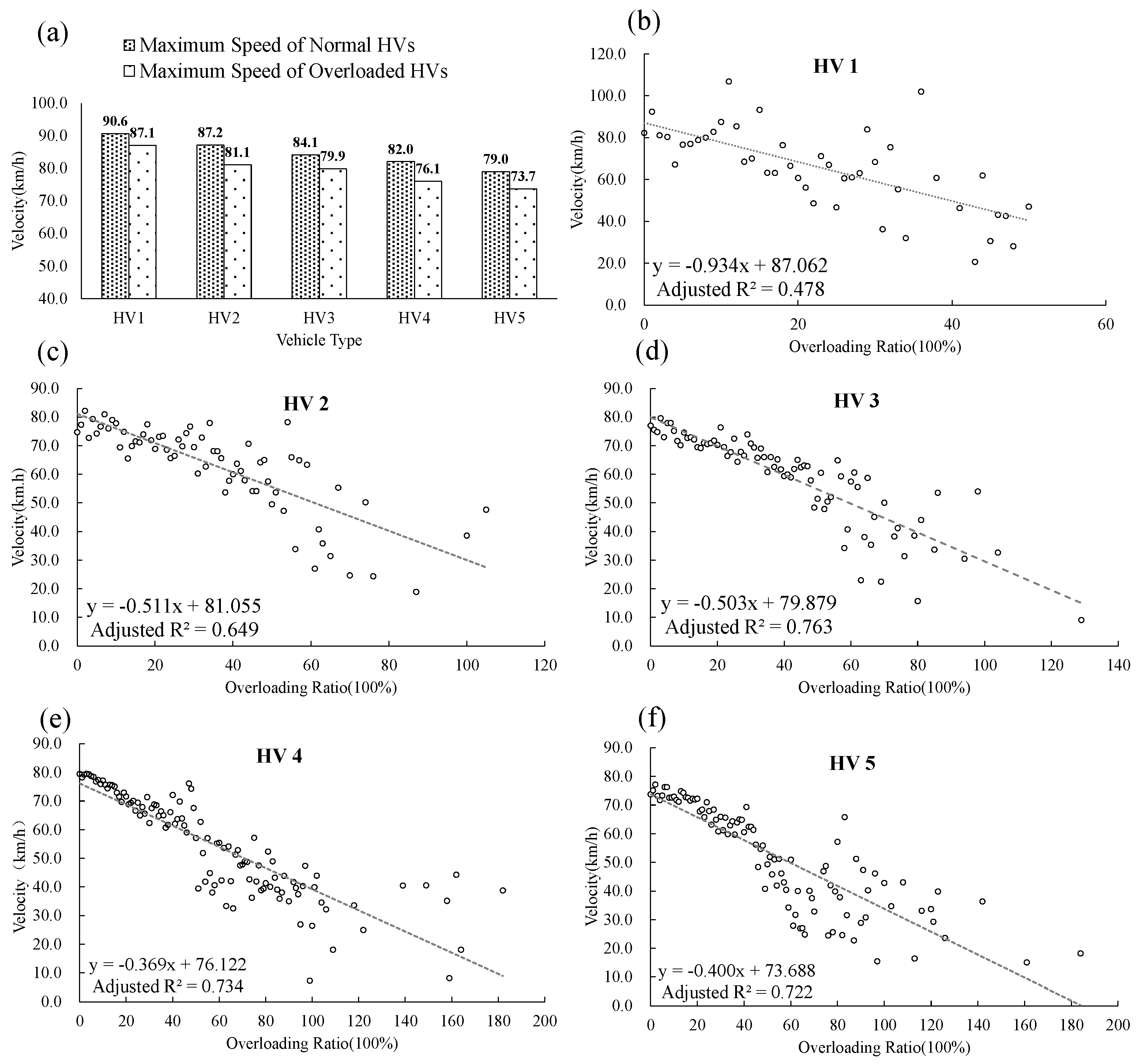
3.3. Overloading Ratio and Maximum Speed

Maximum speed is a significant parameter of traffic flow models, and the maximum speed of heavy vehicles is directly impacted by overloading ratio (i.e., (total weight − weight limit)/weight limit). To analyze the relationship between overloading ratio and maximum speed, the toll station data of HVs with entering and exiting times both between 0:00 and 6:00 a.m. were selected to approximate the free-flow condition. According to the collected data, the maximum speeds decrease with increased vehicle size (as seen in Figure 1a), and the overloaded HVs are slower than the normal ones. The overloading ratio of each HV was aggregated by an increment of 1%. Then, the 90th percentile of the speed in each increment interval was assumed to be the maximum speed for a specific overloading ratio. Lastly, the maximum speeds were regressed by ordinary least squares (i.e., OLS) against the aggregated overloading ratio for each HV type (as seen in Figure 1b–f).

It is obvious that the maximum speed decreases with the increased overloading ratio in each HV type. The statistic results of each regression model are shown in

Table 2. Statistical characteristics of regression coefficients for different HVs.

Vehicle Type	Coefficients		t Stat	P-Value	Lower 95%	Upper 95%	Adjusted R2	F-Statistic	Significance F	Observations
HV1	Constant	87.062	21.592	1.053 × 10−24	78.930	95.194	0.478	39.440	1.430 × 10−07	45
	${\beta }_u$	−0.934	−6.280	1.430 × 1−07	−1.235	−0.634
HV2	Constant	81.055	40.852	4.419 × 10−49	77.095	85.016	0.649	123.983	6.885 × 10−17	69
	${\beta }_u$	−0.511	−11.135	6.885 × 10−17	−0.602	−0.419
HV3	Constant	79.879	50.288	9.353 × 10−62	76.717	83.040	0.763	254.289	2.059 × 10−26	81
	${\beta }_u$	−0.503	−15.946	2.059 × 10−26	−0.566	−0.440
HV4	Constant	76.122	50.173	1.239 × 10−77	73.115	79.129	0.734	303.644	2.033 × 10−33	112
	${\beta }_u$	−0.369	−17.425	2.033 × 10−33	−0.411	−0.327
HV5	Constant	73.688	44.483	2.998 × 10−67	70.401	76.975	0.722	257.511	2.681 × 10−29	101
	${\beta }_u$	−0.400	−16.047	2.681 × 10−29	−0.449	−0.350

. Significance F and P-value of all the five regression models are below than 0.05. The results indicate that the overloading ratio has a significant negative impact on the maximum speed in each HV type. HV1 has a lower adjusted R² value that is smaller than 0.5. The main reason is that there are few overloaded HV1 on the freeway and the overloading ratio is not as large as the other HV types (e.g., the maximum overloading ratio of HV1 is 0.5). It can also be noticed that the fitness is inferior when the overloading ratio is high. The main reason is that there are few samples with high overloading ratio, hence, the 90th percentile of the highest speed could be dispersed. Another potential reason is that the driving behavior of the high overloaded HVs varies greatly. Some drivers realize the danger of overloading and choose to drive at a low speed, while some drive as fast as they can.

The regression results (Table 2) can be used to calculate the maximum speeds of different HV types as the input of the proposed model with considerations for overloaded HVs. The OLS regression model can be represented in its reduced form as:

$$v_{u,\max }^r=g_u(r)=C_u-{\beta }_u\cdot r$$

(2)

where $v_{u,\max }^r$ is the maximum speed of vehicle type u when the overloading ratio is r. C_u and ${\beta }_u$ are the constant and coefficient of vehicle type u, respectively.

It can be found that the constants and ${\beta }_u$ vary from different HV types in Table 2. The constants represent the maximum speeds of each HV type under different overloading ratio, and the regression slopes represent the reduction rate of maximum speeds. The results indicate that HV1 has the highest maximum speed and HV5 has the lowest one when comparing with the other HV types. It is explicable because HV1 and HV5 have the smallest and largest vehicle size and weight capacity, respectively, as seen in Table 1. Meanwhile, the regression slopes (i.e., coefficients) show that HV1 has the highest reduction rate, and the slope appears downtrend when HV has a larger size (i.e., HV2, HV3, HV4, HV5). This is also reasonable because small HVs always have the lower maximum engine power than large HVs, and the maximum speeds of small HVs are more sensitive with the overloading ratio.

4. Multi-Class Traffic Flow Model with Overloaded HVs

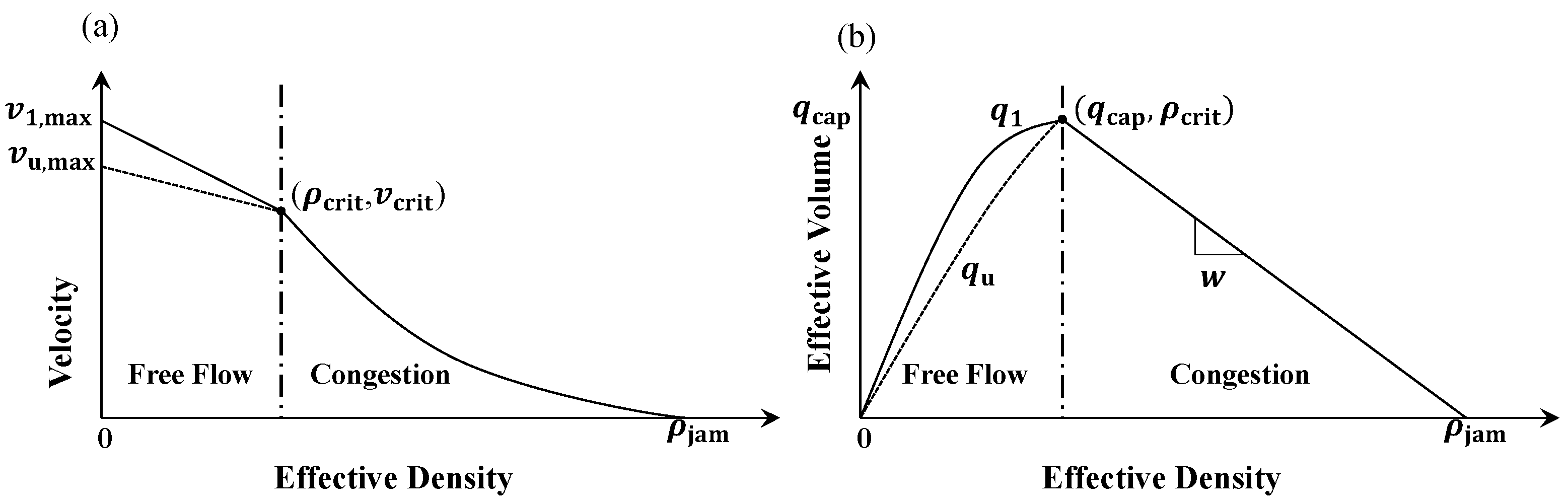
4.1. Multi-Class Fundamental Diagram

In continuous traffic flow, fundamental diagrams are used to describe the relationship of traffic state variables, including speed, density, and volume. Several principles (or assumptions) form the foundation of multi-class continuum traffic flow models to guarantee the existence and uniqueness of the model solution, and several requirements are needed to verify whether the proposed model has qualitatively desirable properties. The principles and requirements are outlined in

Table 3. Principles and requirements of multi-class traffic flow models.

Principles	Requirements
P1. Multi-class traffic flow is a continuous flow.	R1. Given the density of each vehicle type, the class-specific speeds and flows are defined uniquely.
P2. Vehicles are conserved between adjacent segments, and they can only enter or exit through the freeway toll station.	R2. The model has a unique solution on the maximum flow (i.e., capacity).
P3. Traffic flow is a single-pipe flow, and the lane number only affects the segment capacity.	R3. In free flow, the speeds of each vehicle type can be different and are allowed to be constant or decrease with increasing density.
P4. Traffic flow is always in two regimes: free flow or congestion.	R4. In congestion, the speeds of each vehicle type have to decrease monotonously with density, and the speeds should be equal due to car-following driving behavior.
P5. Traffic is always in the equilibrium state.	R5. If the density reaches a certain threshold, the speeds of each vehicle type are all zero.
P6. Traffic consists of homogeneous groups of vehicles and drivers.	R6. If the density is zero, the speeds of each vehicle type are the class-specific free flow speed.

[20,25].

The shape of the fundamental diagram is based on principles and requirements. First, the fundamental diagram should be able to differentiate each vehicle type. Additionally, all the vehicle types should be in the free flow or congestion regime at the same time. Furthermore, in free flow, the speeds of each type can differ. In congestion, they should be equal. Daganzo and Greenshields fundamental diagram cannot satisfy the above principles and requirements. For the Daganzo diagram, the speeds of each vehicle type can differ in free-flow, while it is difficult to guarantee all the vehicle types are in the same traffic condition regime. For the Greenshields diagram, the requirements of the speeds in free-flow and congestion cannot both be guaranteed.

The Smulders fundamental diagram [27] is a combination of the Greenshields fundamental diagram [28] and the Daganzo fundamental diagram [29]. In free-flow, the density-speed panel of the Smulders diagram is identical to the Greenshields diagram, i.e., the speed decreases with increasing density, which is more suitable for empirical data [30]. While in congestion, the density-volume panel of the Smulders diagram is identical to that of the Daganzo diagram, in which the relationship between density and volume is linear. In this study, the Smulders fundamental diagram is chosen as the basis of the freeway multi-class traffic flow model, and the multi-class Smulders fundamental diagram [23] is shown in Figure 2.

Effective density and effective volume are used to represent the average traffic conditions of multi-class traffic flow on one link. The calculation of effective density and effective volume will be discussed in Section 4.4. The multi-class fundamental diagram of the density-speed panel is represented by the following equations.

Free flow ($0\le {\rho }_e<{\rho }_{\mathrm{crit}}$):

$$v_u=v_{u,\max }-\frac{v_{u,\max }-v_{\mathrm{crit}}}{{\rho }_{\mathrm{crit}}}{\rho }_e$$

(3)

Congestion (${\rho }_{\mathrm{crit}}\le {\rho }_e<{\rho }_{\mathrm{jam}}$):

$$v_u=w(\frac{{\rho }_{\mathrm{jam}}}{{\rho }_e}-1)$$

(4)

$$w=\frac{{\rho }_{\mathrm{crit}}{v}_{\mathrm{crit}}}{{\rho }_{\mathrm{jam}}-{\rho }_{\mathrm{crit}}}$$

(5)

where ${\rho }_e$ is the effective density, ${\rho }_{\mathrm{crit}}$ is the critical density, ${\rho }_{\mathrm{jam}}$ is the jam density, subscript u is the vehicle type, $v_u$ is the speed of vehicle type u, $v_{u,\max }$ is the maximum speed of vehicle type u, $v_{\mathrm{crit}}$ is the critical speed, and w is the shockwave speed.

4.2. Definition of Dynamic PCE

The impact of one vehicle on the traffic condition depends on its space occupancy, i.e., the vehicle length plus the space between the two adjacent vehicles [16,24], which is a dynamic variable that changes with speed and headway based on the safe-distance model [31]. This means one vehicle has more influences on traffic condition when it occupies more road space. Moreover, it has been learned that the PCE of HV decreases when the number of HVs increases because the impact of one HV in a platoon is less severe than one in a stream [5,32]. Based on the above discussions, the dynamic PCE of HV class u is defined as a combination of relative space occupancy (i.e., the ratio of space occupancy between class u and passenger car unit) and its proportion to the passenger car:

$${\eta }_{u,i}=f(p_{u,i})\cdot \frac{v_{u,i}\cdot T_{u,i}+L_u}{v_{1,i}\cdot T_{1,i}+L_i}$$

(6)

$$f(p_{u,i})=\frac{1}{1+\alpha \cdot p_{u,i}}$$

(7)

$$p_{u,i}=\frac{N_{u,i}}{N_{1,i}+N_{u,i}}$$

(8)

where the passenger car is represented by u = 1, ${\eta }_{u,i}$ is the dynamic PCE of vehicle type u on link i, $T_{u,i}$ is the headway of vehicle type u on link i (which will be discussed in Section 4.3), $L_u$ is the length of vehicle type u, and $p_{u,i}$ is the proportion of vehicle type u against the total number of the passenger car and vehicle type u (not the total vehicles) on link i. $N_{u,i}$ and $N_{1,i}$ are the number of vehicle type u and passenger cars on link i, respectively. $\alpha$ is the adjustment ratio of the HV proportion, and it was utilized to represent how the influence degree of each HV reduces when the proportion of HVs increases. The appropriate range of the adjusted factor should ensure $f(p_{u,i})\in (0,1]$, so that $\alpha$ ≥ 0.

4.3. Relationship between Vehicle Weight and Minimum Safe Headway

4.3.1. Free-Flow

It is assumed that the brake system of one vehicle type provides the same brake power. The stopping distance of normal and overloaded HVs in free flow, based on the kinetic energy theorem, is represented as follows:

$$S_u=\frac{m_u{v}_u^2}{2F_u};S_u^r=\frac{m_u^r{(v_u^r)}^2}{2F_u}$$

(9)

where u is the vehicle type of HV. $S_u$ and $S_u^r$ are the stopping distance of normal and overloaded HVs, respectively. $m_u$ and $m_u^r$ is the total weight of normal and overloaded HVs. $v_u^{}$ and $v_u^r$ are the travel speed of normal and overloaded HVs, respectively. $F_u$ is the maximum brake force. To avoid a rear-end collision, the minimum safe headway between the rear of the leading vehicle and the head of the following vehicle is represented as:

$$T_u=\frac{S_u}{v_u}=\frac{m_u{v}_u^{}}{2F_u};T_u^r=\frac{S_u^r}{v_u^r}=\frac{m_u^r{v}_u^r}{2F_u}$$

(10)

$$T_u^r=\frac{m_u^r{v}_u^r}{m_u{v}_u}{T}_u$$

(11)

where $T_u$ and $T_u^r$ are the minimum safe headways of normal and overloaded HVs, respectively. According to Equations (2), (3), (11), and set $\frac{m_u^r}{m_u}=r+1$, $T_u^r$ can be written as:

$$T_u^r=(r_{}+1)\cdot \frac{g_u(r){\rho }_{\mathrm{crit}}-[g_u(r)-v_{\mathrm{crit}}]{\rho }_e}{v_{u,\max }^{}{\rho }_{\mathrm{crit}}-(v_{u,\max }-v_{\mathrm{crit}}){\rho }_e}\cdot T_u$$

(12)

4.3.2. Congestion

All the vehicles are assumed to have the same speed in congestion. According to Equation (11), the relationship between the minimum safe headways of normal HVs and overloaded HVs is calculated as follows:

$$T_u^r=\frac{m_u^r}{m_u}{T}_u=(r+1)T_u$$

(13)

4.4. Effective Density and Effective Volume

4.4.1. Effective Density

The effective density of multi-class traffic flow is defined as a weighted sum of the density of each vehicle type:

$${\rho }_{e(i)}^k={\displaystyle {\sum }_u{\eta }_{u,i}^k{\rho }_{u,i}^k}$$

(14)

where ${\eta }_{u,i}^k$ is the dynamic PCE of vehicle type u on link i at time interval k, and ${\rho }_{u,i}^k$ is the density of vehicle type u on link i at time interval k. The calculation of ${\rho }_{u,i}^k$ in this study can be found in Appendix B. The subscripts i and k are omitted for the remainder of this chapter for simplicity.

To use one formula to represent the effective density in both free-flow and in congestion using only known variables, necessary transformations of effective density have been done in Appendix A.1. The boundary conditions on the parameters (i.e., maximum speed and minimum safe headway) are discussed to ensure the existence of a solution to a quadratic equation about effective density and to choose the right root. The detail process can be found in Appendix A. To summarize, the formulation of effective density is:

$${\rho }_e=\frac{(-a_1+{\displaystyle {\sum }_{u}f(p_u){\rho }_u{b}_u})+\sqrt{{(a_1-{\displaystyle {\sum }_{u}f(p_u){\rho }_u{b}_u})}^2+4b_1{\displaystyle {\sum }_{u}f(p_u){\rho }_u{a}_u}}}{2b_1}$$

(15)

where $f(p_u)=\frac{1}{1+\alpha \cdot p_u}$.

In free flow, it is $a_u^f=L_u+T_u{v}_{u,\max }$, $b_u^f=-T_u\frac{v_{u,\max }-v_{\mathrm{crit}}}{{\rho }_{\mathrm{crit}}}$.

In congestion, it is $a_u^c=T_{u}w{\rho }_{\mathrm{jam}}$, $b_u^c=L_u-T_{u}w$;$w=\frac{{\rho }_{\mathrm{crit}}{v}_{\mathrm{crit}}}{{\rho }_{\mathrm{jam}}-{\rho }_{\mathrm{crit}}}$.

When there are overloaded HVs, it is $v_{u,\max }^r=g_u(r)$.

In free flow, it is $T_u^r=(r+1)\cdot \frac{g_u(r){\rho }_{\mathrm{crit}}-[g_u(r)-v_{\mathrm{crit}}]{\rho }_e}{v_{u,\max }^{}{\rho }_{\mathrm{crit}}-(v_{u,\max }-v_{\mathrm{crit}}){\rho }_e}\cdot T_u$.

In congestion, it is $T_u^r=(r+1)T_u$.

4.4.2. Effective Volume of Multi-Class Traffic Flow

After getting the effective density, the speed of vehicle type u (i.e., $v_u^{}$) can be calculated using Equations (3) or (4). Then, the dynamic PCE (i.e., ${\eta }_u^{}$) also can be obtained. At last, the effective volume of vehicle type u (i.e., $q_{e(u)}^{}$), can be calculated using the following equation:

$$q_{e(u)}^{}={\eta }_u^{}\cdot {\rho }_u^{}\cdot v_u^{}$$

(16)

The total effective volume on link i is the sum of all types of vehicles:

$$q_e^{}={\displaystyle {\sum }_u{q}_{e(u)}^{}}$$

(17)

5. Validation of Model Results

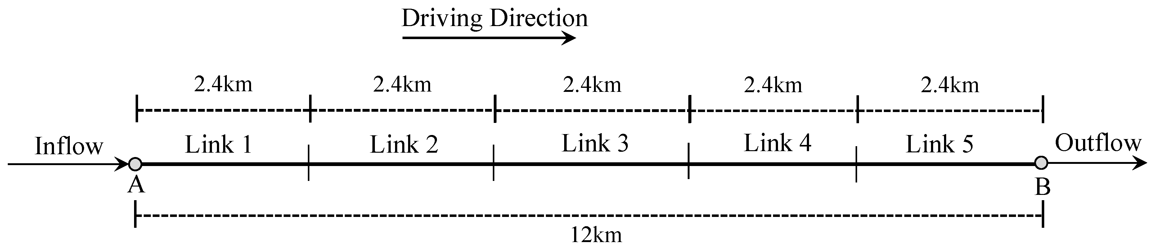
5.1. Model Preparation

A segment of G15 freeway in Jiangsu Province, China was selected to evaluate the model performance empirically. The segment connects a mainline toll station named Sulu station and its adjacent ramp toll station named Haitou station. The analyzed travel direction is from the mainline toll station to the ramp toll station. The total travel distance is 28 km, and there are two lanes in the travel direction. In addition, there is no other on/off ramp or service area between these two toll stations, so all the vehicles that entered the selected segment can be captured by toll station data from the mainline.

All of the parameters are shown in

Table 4. Parameters of the model.

Parameters	Unit	Definition	PC1	HV1	HV2	HV3	HV4	HV5
$L_u$	m	the vehicle length of type u	5	4	5	7	12	13
$v_{u,\max }$	km/h	the maximum speed of type u	117.5	90.6	87.2	84.1	82.0	79.0
$v_{u,\max }^{\mathrm{w}}$	km/h	the maximum speed of overloaded type u		87.1	81.1	79.9	76.1	73.7
$T_u$	s	the minimum safe headway of type u	1	1	1.5	2	2.5	2.5
$q_{\mathrm{crit}}^{}$	pce/h/ln	the capacity of single lane	2200
$v_{\mathrm{crit}}$	km/h	the critical speed	60
${\rho }_{\mathrm{crit}}$	pce/m/ln	the critical density	0.037
${\rho }_{\mathrm{jam}}$	pce/m/ln	the jam density	0.2
α	unit	adjustment ratio of proportion	0.93

. The parameters of each vehicle type are based on the results of Table 1, and the parameters of the freeway segment are obtained from HCM 2010 [5] and the Jiangsu Freeway Traffic Condition Analyzing Report [4].

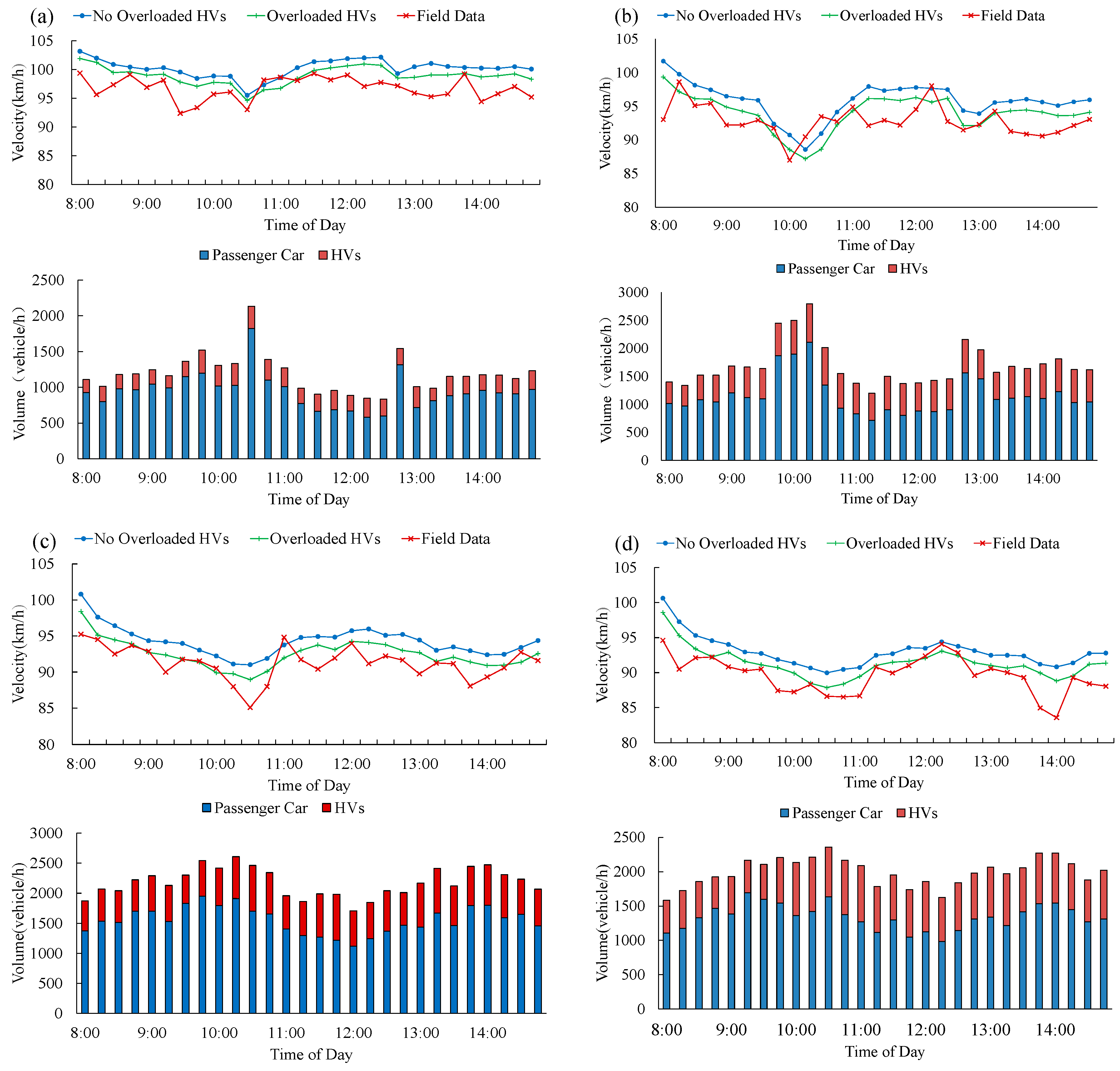
5.2. Model Results versus Real Traffic Data

The freeway segment suffers from high heavy vehicle volumes on Monday and Friday each week, and the peak hour ranges from 9:00 a.m. to 14:00 p.m. In order to evaluate the proposed model performance both in weekday and weekend, the real traffic data from July 1st (Sunday), 2nd (Monday), 4th (Wednesday), and 27th (Friday) of 2012 were chosen for model validation. The analyzing time period was from 8:00 a.m. to 15:00 p.m., which covers the AM peak and PM peak of the selected segment. The time interval was 15 min, which is widely used in traffic management and time-dependent traffic condition analysis. Because the initial network is empty, the demand loading time should be prior to the analyzing time period, otherwise, the model will cause the prediction of an unrealistically higher travel speed. In this practical application, the demand loading started at 6:30 a.m., and then the extract the time period of 8:00 a.m.–15:00 p.m. took place to evaluate the model performance.

In the first model run, overloaded HVs were treated as normal HVs. In the second model run, overloaded HVs and the normal ones were separated. The overloading ratio of each HV may be different. In order to obtain the overloading ratio r in Equation (2) for each time interval, the overloading ratio was averaged within each time interval by freeway toll data, and then the maximum speed of overloaded HVs was calculated using the regression model in Equation (2). The field data was calculated using Equation (1), and the travel times of PC1 were converted into speed for comparison in Figure 3.

As seen in Figure 3, the proposed model can represent the time-dependent speed variation of PC1 when compared with the field data, and the difference between the results when considering the overloaded HVs or not can be observed.

Analysis of variance (ANOVA) is implemented to check whether considering the overloaded HVs makes differences on the traffic condition of the freeway segment. Set α = 0.05, and the results are shown in

Table 5. Analysis of variance about the model results considering overloaded HVs or not.

Test Date	Mean Square Error	F	P-Value	Fcrit
1 July	26.841	10.370	0.002	4.020
2 July	45.108	6.096	0.017	4.020
4 July	43.507	11.180	0.002	4.020
27 July	37.815	7.874	0.007	4.020

.

It can be found that the F-values of the four test days are all larger than F_crit, and P-values are all below 0.05. The results indicate that there are significant differences on traffic condition when considering the overloaded HVs or not.

Based on the proposed multi-class traffic flow model in Section 4, the free flow speed and minimum safe distance are affected by the overloading ratio. Then, the dynamic PCE changes based on the space occupancy of the overloaded HVs. Finally, the effective density is affected, and the travel speed of each vehicle type changes based on the calibrated multi-class traffic flow diagram. When considering the overloaded HVs, the effective density will be a bit higher and the travel speed will be lower. It is noticeable that speed values are different between the overloaded HVs and non-overloaded HVs model, but not the changing trend. Since these two models are both based on the Smulders fundamental diagram, the speed curves with/without consideration for overloaded HVs will be similar unless there is an extremely high proportion of overloaded HVs with high overloading ratio.

Mean absolute percentage error (MAPE) was used to evaluate the accuracy of the model results (

Table 6. Characteristics of traffic demand and the MAPE of model results.

Date	Average Volume (Vehicle/h)						Overloading Proportion of HVs (%)	MAPE
	PC1	HV1	HV2	HV3	HV4	HV5		No Overloaded HVs	Overloaded HVs	MAPE Reduction
1 July	883	47	70	48	28	48	16.2%	3.78%	2.08%	45.0%
2 July	1083	114	199	81	47	101	13.9%	3.66%	2.50%	31.7%
4 July	1195	118	186	113	71	114	17.3%	3.34%	1.72%	48.5%
27 July	1251	119	205	118	55	160	15.8%	3.58%	2.38%	33.5%

):

$$\mathrm{MAPE}=\frac{100\%}{n_T}{\displaystyle {\sum }_{i=1}^{n_T}\left|\frac{V_{M(i)}-V_{A(i)}}{V_{A(i)}}\right|}$$

(18)

where $V_{M(i)}$ is the model result of travel speed during time interval i, $V_{A(i)}$ is the actual travel speed during time interval i, and $n_T$ is the number of time intervals.

It can be found that the MAPE improved when there were overloaded HVs. The reduction of MAPE was more than 30% during the four testing days. When the overloading proportion of HVs was higher, the reduction of MAPE was more significant. The results show that the proposed model can represent the traffic conditions more realistically when considering for overloaded HVs. When the overloading performance is serious, the traffic condition will be overrated by traditional models that treat overloaded HVs as normal ones, and this will lead to heavy traffic congestion in reality. Thus, the freeway traffic managers cannot evaluate the accurate traffic condition, which may lead to inappropriate traffic management strategies. In China, the freeway toll data include vehicle type, vehicle weight, total weight limit, etc., which provides the data fundamental for the proposed model on practical application. However, there are still some time intervals suffering a relatively large gap, although the model results fit the field data for the overall trend. This is mainly caused by the factors affecting the traffic conditions that have not been considered in the proposed model, e.g., the lane-changing behavior of different vehicles, weather condition, and other stochastic disturbances. All of these will lead to the deviation, and improvements can be considered in further studies.

Moreover, to analyze the impact of overloaded HVs on traffic conditions in different demand and supply combinations, several scenario tests were conducted and are discussed in Section 6.

6. Model Scenario Test

6.1. Preparation of the Scenario Test

To identify the impacts of overloaded HVs on traffic conditions, a simple freeway segment type without merge/diverge was chosen in this simulation test. The freeway basic segment is 12 km with two lanes. It is split evenly into five links, and each link is 2.4 km long. All the vehicles entered the freeway segment from station A, and then left from station B (Figure 4). The analysis time interval was 1 min and the total time period was 30 min. The freeway segment was empty at initial status. Only PC1 and HV5 were represented in this scenario test, and all the parameters were the same as in Table 4.

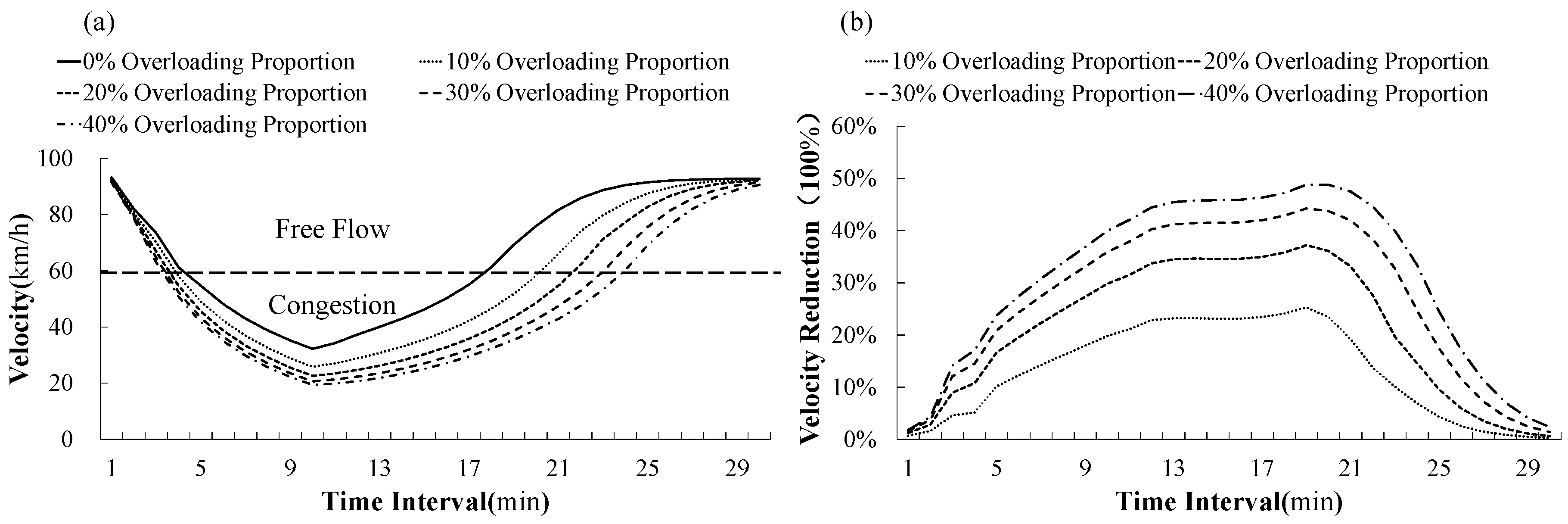
6.2. Scenario 1: Impact of the Overloading Proportion

Scenario 1 aims to exhibit the impact of overloaded HVs when the overloading proportion (i.e., the number of overloaded HVs/ the total number of HVs) changes. The flow rate of passenger cars was 3500 veh/h for the entire testing time period. The inflow rate of HVs was 1500 veh/h during the first 10 min, then this dropped to zero immediately, and the overloading ratio was fixed as 25%. The only changing variable was the overloading proportion, which ranges from 0 to 40%. The speed variation of PC1 on link 1 is shown in Figure 5.

As seen in Figure 5, passenger car speeds decreased with increasing overloading proportions. Compared with the situation when there was no overloaded HV, the maximum speed reduction ratio was 48.8% when the overloading proportion was 40%. Meanwhile, when the overloading proportion was higher, the duration of congestion was longer. For instance, the length of the congestion period was 19 or 23 min when the overloading proportion was 10 or 40%, respectively.

It is also noticeable in Figure 5b that the first 10% of overloaded HVs brought the most negative impacts. The maximum speed reduction was 25.3% when the overloaded proportion was 10%. However, when the overloaded proportion increased to 20%, the maximum speed reduction was 37.2%. This is less than 50.6% (i.e., the double of 25.3%), meaning that although the total impacts increased with increasing overloaded proportions, the average impact of each overloaded HV decreased. This is consistent with Highway Capacity Manual (HCM 2010) [5] that “when there are more HVs on a freeway, the HVs could form platoons and have less interaction with passenger cars”.

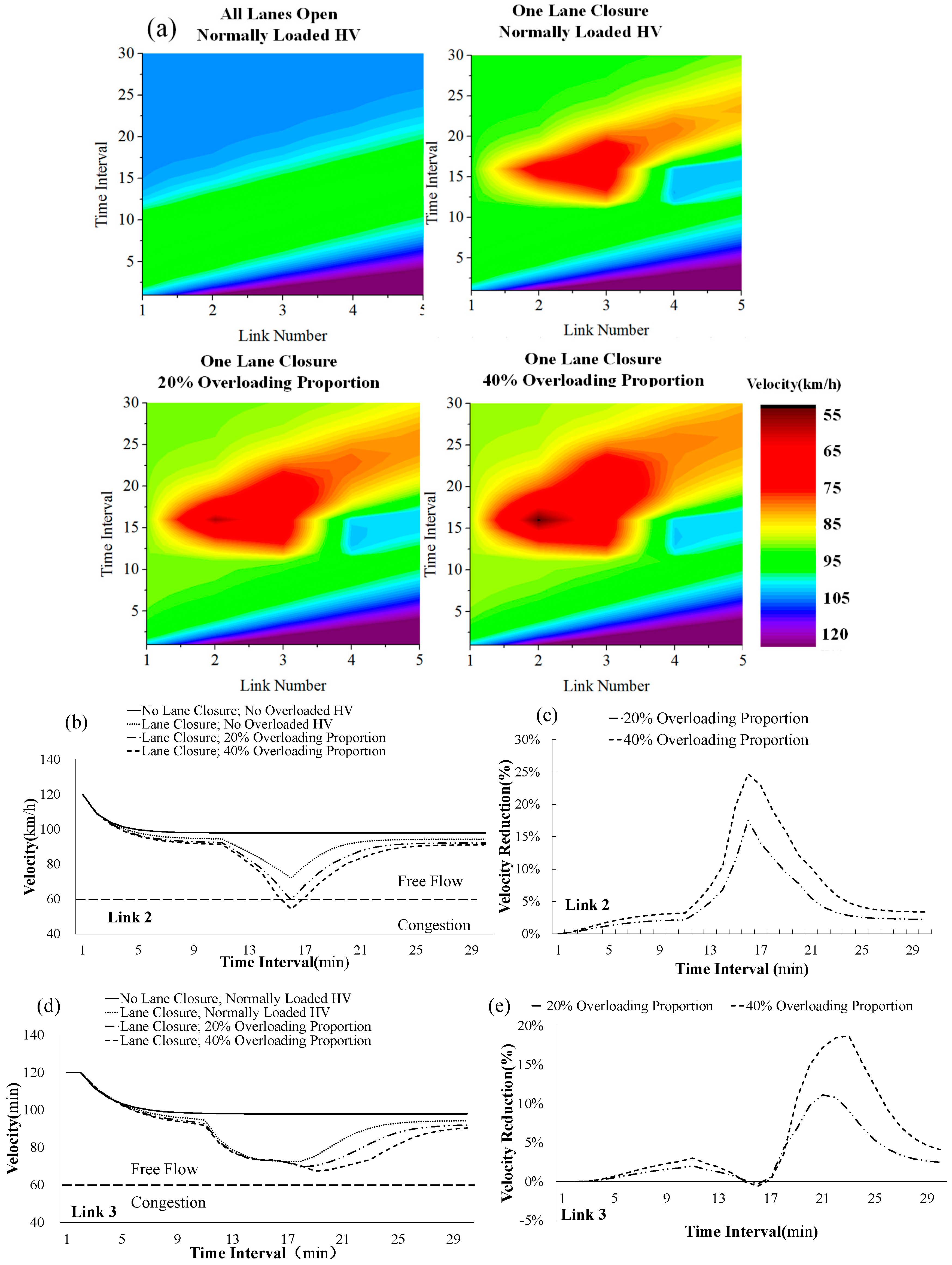
6.3. Scenario 2: Impact of the Overloaded HVs at Work Zones

Scenario 2 aims to represent the impact of overloaded HVs on traffic conditions around work zones. A work zone located on link 3 caused one lane closure from the 11th minute to the 15th minute, i.e., the capacity of link 3 reduced by half. The flow rates of passenger cars and HVs were both fixed throughout the entire time period at 2000 and 1000 veh/h, respectively. In this scenario, the only changing variable is the overloading proportion, and the overloading ratio is fixed as 25%. The traffic flow propagation method is discussed in Appendix B. The speed variation of PC1 is shown in Figure 6.

As seen in Figure 6a, when one lane was closed and no overloaded vehicle exists, link 3 suffered from capacity reduction and the speed of passenger cars decreased at first. Meanwhile, link 2 suffered from a lower outflow rate due to the capacity reduction of link 3. The inflow of link 4 and link 5 became smaller, therefore, their traffic conditions were better. When the closed lane on link 3 opened again at the 16th minute, the residual vehicles on link 2 entered link 3 with a larger inflow rate, so link 3 still suffered from poor traffic conditions, although its capacity recovered. These vehicles kept driving through the downstream links and led to worsen traffic conditions on link 4 and link 5 after the closed lane opened.

As seen in Figure 6b–d, the congestion became more serious when the overloading proportion increased, especially on link 2 and link 3. Compared with the situation without overloaded HVs, the lowest speed on link 2 and link 3 decreased 24.7 and 6.5%, respectively, and the low speed duration under 80 km/h on link 2 and link 3 increased 98 and 51%, respectively, when the overloading proportion was 40%. It can be found that the travel speeds of all vehicles were lower when there were more overloaded HVs. Additionally, it took more time for the overloaded HVs to drive through the work zone, and they caused a longer congestion duration. Meanwhile, there were more overloaded HVs stocked on link 2 due to the capacity reduction on link 3, when the proportion of overloaded HVs increased. This explains why link 2 suffered from the largest speed reduction.

6.4. Policy Suggestions

The results of the above two scenarios show that the congestion level becomes worse and congestion duration increases with the overloading proportions. This indicates that the existing overloaded HVs do not only cause pavement damage but also lead to low travel speed and an inferior level of service, especially when capacity drop (i.e., work zone) exists. Therefore, it is recommended that overloaded HVs should be forbidden, and the penalty of overloaded HVs should both consider pavement damage and traffic condition influences.

7. Conclusions and Recommendations

Overloaded HVs impose significant impacts on traffic conditions due to their inferior driving performance. However, few existing analytical tools properly address the impact of overloaded HVs on a large-scale network for the online application. In this study, the relationship between overloading ratio and travel speed of overloaded HVs has been analyzed using field data. A new dynamic PCE based on space occupancy was designed for the overloaded HVs, and it can represent the different influences of overloaded HVs when the traffic condition changes. Finally, a new multi-class kinematic wave traffic flow model based on dynamic PCE and the Smulders fundamental diagram was proposed with considerations for the existence of overloaded HVs. Meanwhile, the existence and uniqueness of effective density and the effective volume of the proposed multi-class traffic flow model was proven.

The results of the proposed model are valid. The empirical study shows the model can represent actual traffic conditions, and the model is more accurate with considerations for the existence of overloaded HVs. The improvements in accuracy increase when there are more overloaded HVs. Moreover, the results of scenario tests are plausible, and they show that the increase of the overloading proportion leads to larger speed reductions and longer congestion durations. The proposed model can be used for the online estimation of freeway traffic conditions with considerations for overloaded HVs. It also can help authorities determine traffic management strategies accordingly.

However, there are several improvements that could be implemented in further studies. First, a multi-level model instead of several separate models for each HV type may be more appropriate on the regression between maximum speed and overloading ratio. Meanwhile, the proposed model can be extended to a multi-lane version to describe vehicle interaction during lane changing. Moreover, the dynamic PCE includes the proportion of HVs and a fixed adjustment parameter is used. Other functions could be made to represent the relationship between PCE and vehicle type proportion better. Furthermore, the space occupancy function could be improved by incorporating other advanced car-following models. Additionally, how to obtain and update the multi-class traffic flow parameters with different environmental conditions will be a future study direction.

References

1. Ren, Y.; Wu, S. Analysis of heavy trucks’ effect on freeway traffic safety. In Proceedings of the 2011 International Conference on Electronic and Mechanical Engineering and Information Technology (EMEIT), Harbin, China, 12–14 August 2011. [Google Scholar]
2. Xiao, R.; Li, B.; Chen, Y. Trend analysis of expressway transportation based on big data. J. Traffic Transp. Eng. 2015, 117, 85–90. [Google Scholar]
3. Han, W.; Wu, J.; Cai, C.S.; Chen, S. Characteristics and dynamic impact of overloaded extra heavy trucks on typical highway bridges. J. Bridge Eng. 2014, 20, 05014011. [Google Scholar] [CrossRef]
4. Zhou, H.W.; Li, G.X.; Shi, K.T. Jiangsu Freeway Traffic Condition Analyzing Report; Jiangsu Freeway Network Operation & Management Center: Nanjing, China, 2012. [Google Scholar]
5. Manual, H.C. HCM2010. In Transportation Research Board; National Research Council: Washington, DC, USA, 2010. [Google Scholar]
6. Aghabayk, K.; Sarvi, M.; Young, W. A macroscopic study of heavy vehicle traffic flow characteristics. In Proceedings of the ARRB Conference, Perth, Australia, 23–26 September 2012. [Google Scholar]
7. Aghabayk, K.; Sarvi, M.; Young, W. Understanding the dynamics of heavy vehicle interactions in car-following. J. Transp. Eng. 2012, 138, 1468–1475. [Google Scholar] [CrossRef]
8. Abdullah, A.S. Development of Integrated Weigh-in-Motion System and Analysis of Traffic Flow Characteristics considering Vehicle Weight; The University of Tokushima Japan: Tokushima, Japan, 2011. [Google Scholar]
9. Saifizul, A.A.; Yamanaka, H.; Karim, M.R. Empirical analysis of gross vehicle weight and free flow speed and consideration on its relation with differential speed limit. Acc. Anal. Prev. 2011, 43, 1068–1073. [Google Scholar] [CrossRef] [PubMed]
10. Dhamaniya, A.; Chandra, S. Concept of Stream Equivalency Factor for Heterogeneous Traffic on Urban Arterial Roads. J. Transp. Eng. 2013, 139, 1117–1123. [Google Scholar] [CrossRef]
11. Cao, N.Y.; Sano, K. Estimating capacity and motorcycle equivalent units on urban roads in Hanoi, Vietnam. J. Transp. Eng. 2012, 138, 776–785. [Google Scholar] [CrossRef]
12. Geistefeldt, J. Estimation of passenger car equivalents based on capacity variability. Transp. Res. Rec. 2009, 2130, 1–6. [Google Scholar] [CrossRef]
13. De Luca, M.; Dell’Acqua, G. Calibrating the passenger car equivalent on Italian two line highways: A case study. Transport 2013, 29, 1–8. [Google Scholar]
14. Ahmed, U.; Drakopoulos, A.; Ng, M. Impact of Heavy Vehicles on Freeway Operating Characteristics under Congested Conditions. Transp. Res. Rec. 2013, 2396, 28–37. [Google Scholar] [CrossRef]
15. Mehar, A.; Chandra, S.; Velmurugan, S. Passenger Car Units at Different Levels of Service for Capacity Analysis of Multilane Interurban Highways in India. J. Transp. Eng. 2013, 140, 81–88. [Google Scholar] [CrossRef]
16. van Lint, J.W.C.; Hoogendoorn, S.P.; Schreuder, M. Fastlane: New Multiclass First-Order Traffic Flow Model. Transp. Res. Rec. 2008, 2088, 177–187. [Google Scholar] [CrossRef]
17. Ngoduy, D. Multiclass first-order traffic model using stochastic fundamental diagrams. Transportmetrica 2011, 7, 111–125. [Google Scholar] [CrossRef]
18. Bellomo, N.; Dogbe, C. On the modeling of traffic and crowds: A survey of models, speculations, and perspectives. SIAM Rev. 2011, 53, 409–463. [Google Scholar] [CrossRef]
19. Logghe, S.; Immers, L.H. Multi-class kinematic wave theory of traffic flow. Transp. Res. Part B Methodol. 2008, 42, 523–541. [Google Scholar] [CrossRef]
20. Del Castillo, J.M. Three new models for the flow–density relationship: Derivation and testing for freeway and urban data. Transportmetrica 2012, 8, 443–465. [Google Scholar] [CrossRef]
21. Daganzo, C.F. A behavioral theory of multi-lane traffic flow. Part I: Long homogeneous freeway sections. Transp. Res. Part B Methodol. 2002, 36, 131–158. [Google Scholar] [CrossRef] [Green Version]
22. Chanut, S.; Buisson, C. Macroscopic model and its numerical solution for two-flow mixed traffic with different speeds and lengths. Transp. Res. Rec. 2003, 1852, 209–219. [Google Scholar] [CrossRef]
23. Ngoduy, D.; Liu, R. Multiclass first-order simulation model to explain non-linear traffic phenomena. Phys. A Stat. Mech. Appl. 2007, 385, 667–682. [Google Scholar] [CrossRef]
24. Van Wageningen-Kessels, F.; Van Lint, H.; Hoogendoorn, S.; Vuik, K. A New Generic Multi-class Kinematic Wave Traffic Flow Model: Model Development and Analysis of Its Properties. Transportation 2014, 29, 449–456. [Google Scholar]
25. Van Wageningen-Kessels, F. Multi-Class Continuum Traffic Flow Models: Analysis and Simulation methods. Ph.D. Thesis, Delft University of Technology/TRAIL Research School, Delft, The Netherlands, 2013. [Google Scholar]
26. Wang, X.; Chen, X. Travel time estimation of a single segment based on freeway toll data. In Proceedings of the 14th COTA International Conference of Transportation Professionals: Safe, Smart, and Sustainable Multimodal Transportation Systems, CICTP 2014, Changsha, China, 4–7 July 2014; pp. 2161–2174. [Google Scholar]
27. Smulders, S. Control of freeway traffic flow by variable speed signs. Transp. Res. Part B Methodol. 1990, 24, 111–132. [Google Scholar] [CrossRef]
28. Qu, X.; Zhang, J.; Wang, S. On the stochastic fundamental diagram for freeway traffic: model development, analytical properties, validation, and extensive applications. Transp. Res. Part B Methodol. 2017, 104, 256–271. [Google Scholar] [CrossRef]
29. Daganzo, C.F. The cell transmission model: A dynamic representation of highway traffic consistent with the hydrodynamic theory. Transp. Res. Part B Methodol. 1994, 28, 269–287. [Google Scholar] [CrossRef]
30. Qu, X.; Wang, S.; Zhang, J. On the fundamental diagram for freeway traffic: A novel calibration approach for single-regime models. Transp. Res. Part B Methodol. 2015, 73, 91–102. [Google Scholar] [CrossRef]
31. Yang, D.; Jin, P.; Pu, Y.; Ran, B. Safe distance car-following model including backward-looking and its stability analysis. Eur. Phys. J. B 2013, 86, 92. [Google Scholar] [CrossRef]
32. Marlina, S. Understanding the Dynamics of Truck Traffic on Freeways by Evaluating Truck Passenger Car Equivalent (PCE) in the Highway Capacity Manual (HCM) 2010; University of Colorado at Denver: Denver, CO, USA, 2012. [Google Scholar]
Figure 1. (a) Difference of the maximum speed between overloaded HVs and normal HVs. (bf) Relationship between the maximum speeds and overloading ratio among different types of HVs.
Sustainability 10 04694 g001
Figure 2. Multi-class traffic flow fundamental diagram. (a) Density–speed panel. (b) Density–volume panel.
Sustainability 10 04694 g002
Figure 3. Comparison of passenger car travel speed from model results and field data on (a) Sunday; 1 July 2012; (b) Monday, 2 July 2012; (c) Wednesday, 4 July 2012; and (d) Friday, 27 July 2012.
Sustainability 10 04694 g003
Figure 4. Test a single freeway segment.
Sustainability 10 04694 g004
Figure 5. (a) Speed with different overloading proportions on link 1. (b) Speed reduction with different overloading proportions on link 1.
Sustainability 10 04694 g005
Figure 6. (a) Speed variations on both spatial and temporal dimensions. (b) Speed on link 2. (c) Speed reduction on link 2. (d) Speed on link 3. (e) Speed reduction on link 3.
Sustainability 10 04694 g006