Weather Risk–Reward Contract for Sustainable Agri-Food Supply Chain with Loss-Averse Farmer

Abstract

Compared with the traditional agri-food supply chain (AFSC) whose only goal is to maximize economic benefits, the sustainable agri-food supply chain (SAFSC) starts to attract more attention. Typical challenges faced by SAFSC development are unfair pricing of produce, yield uncertainty caused by adverse weather, as well as conflict and cooperation between stakeholders and sustainable activities of SAFSC. In this paper, we establish a two-echelon decision-making model consisting of a loss-averse farmer and a loss-neutral company. A guaranteed price mechanism is contrived to mitigate the effects of uncertain procurement price on the farmers’ profit. It is found that this mechanism can improve the sustainable investment level but fails to reach the optimal level of the SAFSC system. Thus, a risk–reward contract taking into account the weather index (temperature) and the degree of loss aversion is designed. Results show that this contract can settle the distortion of the sustainable investment level and effectively motivate farmers to participate in the sustainable agricultural practice. Furthermore, we derive the conditions on the contract parameters under which both the company and the farmer are motivated to exert efforts to stand by sustainable agricultural practice.

1. Introduction

With worldwide awareness of sustainable development, the traditional agri-food supply chain (AFSC) focusing only on economic benefits is being re-scrutinized. It faces severe and complex challenges: how to balance economic benefits, environmentally friendly practices, and social welfare in the process of development [1]. Therefore, the development of AFSC should abide by the idea of sustainable development, paying more attention to the triple bottom line (TBL): profit (economic aspect), planet (environmental aspect), and people (social aspect) [2].

Due to increasingly strict requirements imposed by laws and regulations, many companies from different countries or regional areas have subscribed to the practice of sustainable agri-food supply chain (SAFSC) operations. For example, Italian company Barilla offers partially-guaranteed-price (PGP) contracts to farmers to encourage them to comply with sustainable agricultural practice [3]. Consequently, the reduction of carbon footprint caused by Barilla is 30%, the farmers’ production cost is lowered by 30%, and the increase in farmers’ production yield is 20% [4]. To deal with the unfair pricing situation where sales middlemen could force farmers to sell their produce at a low price, the Indian government promulgated the Agricultural Production Marketing Act, which enables farmers to sell their produce through auction. In accordance with the Act, Indian Tobacco Corporation (ITC) Limited initiated e-Choupals (that uses information and communications technology to change selling operations for the farmers in India) to address unfair pricing of produce, which in turn safeguarded farmers’ interests [5]. To alleviate poverty among farmers caused by unemployment and to protect the environment deterioration due to deforestation for grain plots in rural areas, the Bhutanese government encourages farmers to plant high-value hazelnut trees. The growing of hazelnut trees has provided employment opportunities for farmers. It has also created economic benefits for farmers and the concerned company, Mountain Hazelnuts. Furthermore, the growing of hazelnut trees has enabled the achievement of returning the grain plots to forestry and grass, resulting in the sustainable development of the local agro-ecological environment [6].

The implementation of sustainable operating practices has propelled a theoretical exploration of the sustainable supply chain (SSC) among scholars and experts [7]. Tang et al. designed the partially-guaranteed-price contracts between farmers and agri-food companies and found that a price premium can stimulate the farmers to exert efforts to comply with sustainable agricultural practices [4]. However, their work gives no considerations to the weather risk encountered in agricultural production activities. In comparison with the sustainable development of traditional SCs, some experts studied the more complicated and severe challenges of SAFSCs, such as increased greenhouse gas emissions during agricultural production and processing [8], unfair procurement prices of produce frequently faced by farmers [5,9], mismatch between the supply and demand for some agricultural products [10], increasing awareness of safety food requirements among customers [11], and poverty caused by underemployment of small farm households in developing economies [6]. Even though there has been some work done to identify the attributes of sustainability in AFSC, few effort has been made to consider adverse weather factors in SAFSC and to come up with a holistic framework keeping a balance among economic, social, and environmental challenges.

Consequently, this paper intends to address this gap. In fact, few research has considered all three pillars (economy, environment, society) of sustainability in SAFSC using an optimization approach. This paper, considering all three dimensions of sustainability, studies the two-level agri-food supply chain system consisting of a lose-neutral company and a loss-averse farmer and with the aim at designing effective contracts to stand by sustainable agricultural practice. To the best of our knowledge, this paper is the first to take into consideration unfair pricing of produce, yield uncertainty caused by adverse weather, as well as conflict and cooperation between stakeholders in sustainable activities in SAFSC management. Furthermore, this work shows that using weather risk–reward contracts can settle the distortion of the sustainable investment level and effectively incentive farmers to participate in the sustainable agricultural practice.

The rest of this paper is organized as follows. In Section 2, background and literature review of this paper is given. In Section 3, we give the model preliminaries and construct the model. In Section 4, we provide the guaranteed price mechanism for expanding the farmers’ margin: farmers’ decision on sustainable investment level is in Section 4.1, company’s decision on guaranteed price is in Section 4.2, and comparative analysis of sustainable investment level is in Section 4.3. We design the weather risk–reward contract for improving sustainable investment level in Section 5. Finally, we conclude this paper with discussion focusing on managerial insights and the limitations of this study in Section 6.

2. Background and Literature Review

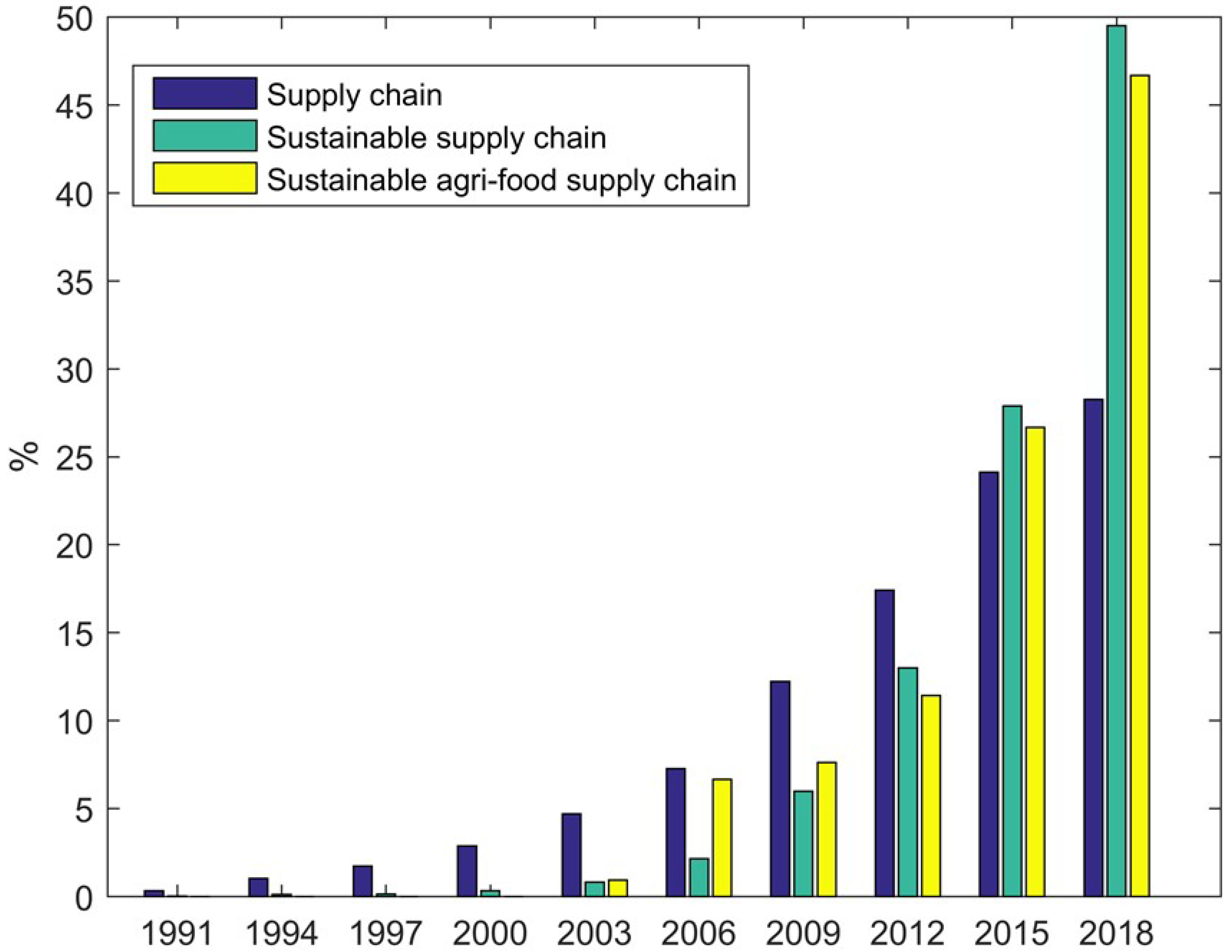
To exam the research trend of SAFSC, we searched the academic articles published from January 1991 to July 2018 using the Web of Science (Web of Science connects publications and researchers through citations and controlled indexing in curated databases spanning every discipline. Use cited reference search to track prior research and monitor current developments in over 100 years’ worth of content that is fully indexed, including 59 million records and backfiles dating back to 1898) citation database. By entering “supply chain”, “sustainable supply chain”, and “sustainable agri-food supply chain”/“sustainable agro-food supply chain”/“sustainable food supply chain” in the searching boxes of topic, title or keyword on the databases of the Web of Science, we can see from Figure 1 the research trends of the supply chain (SC), sustainable supply chain (SSC), and SAFSC in the latest twenty years. Analysis of Figure 1 reveals that the number of research articles in SC is increasing at a slower rate or remains the same if excluding the interference factor caused by yearly increase in the number of journals included in the databases of the Web of Science. The number of papers on SSC is exponentially increasing since 2000, which means that SC integrated with sustainable development has become an emerging research area. Moreover, the number of papers on SAFSC started to increase exponentially from 2003, which means that SAFSC has started to be recognized by scholars and experts in the field of SC as an emerging research area.

Due to the differences in food systems between different countries or regional areas, the relevant study of SAFSC is clearly imbalanced, with a majority of published papers based on individual country-specific issues. On the whole, the developed countries have been popularly examined while developing countries have not been well-explored in terms of the social and environmental dimensions of AFSC [4]. One possible reason is that the study of AFSC of developing countries focuses mainly on the economic objectives, such as how to increase food again to feed the population, while ignoring the environmental and social factors of AFSC [7].

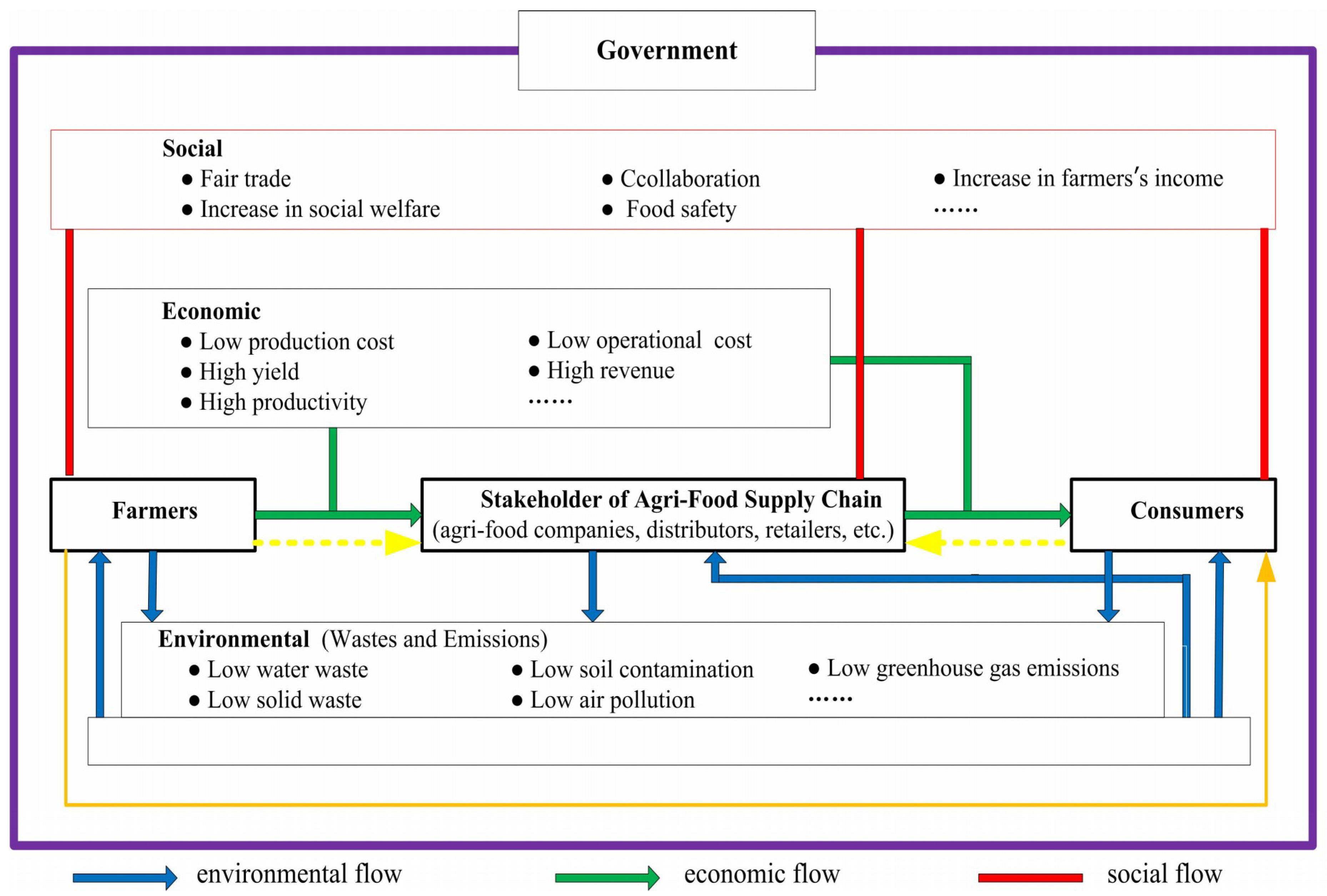
Whether for developed countries or for developing countries, the study of SAFSC needs to consider the ecosystem of the AFSC. Following Tang et al.’s the conceptual framework of the PPP ecosystem (profit, planet, people) [12], a sustainable ecosystem of the AFSC is constructed, as shown in Figure 2, to relate the challenges from the concrete elements in economy, environment, and the society in the SAFSC development.

As shown in Figure 2, the AFSC sustainable ecosystem consists of the flow of three major elements: the financial flow (economic aspect), the development flow (social aspect), and the resource flow (environment aspect). There are four essential bodies which are the government, farm households, core stakeholders of the AFSC (including agriculture related enterprises, distributors, and retailers), and customers. First, core stakeholders of the AFSC and farm households utilize natural resources like water, land, and air (blue up arrows) to produce or process agricultural products to meet customer needs at the agricultural products market. Meanwhile, waste and discharges are generated in the process of produce production, circulation, and processing (blue down arrows). Second, different from the traditional AFSC which only focuses on economic benefits by minimizing cost or maximizing benefits (green arrows), core enterprises of SAFSCs need to shoulder more social responsibilities (red rectangle) and are pressed to pay more attention to their social and environmental responsibilities. Third, to ensure the sustainable development of the ecosystem, SAFSC leaders need to help lift poor farmers out of poverty so that they become customers with purchasing power (orange arrow) [13]. For example, Nestlé has initiated several rural area development programs to help farmers out of poverty and become potential customers, which in turn contributes to Nestlé reaping benefits [12]. Finally, the government exerts an influence on every aspect of the sustainability of the AFSC ecosystem. It usually formulates effective policies like trading policies and taxing policies to regulate the behavior of AFSC stakeholders, farmers, and customers, and encourages them to assume their environmental and social responsibilities while reaping economic benefits [12].

On the basis of the analysis of SAFSC research trends (Figure 1) and the description of the sustainability of the AFSC ecosystem (Figure 2), we will, in what follows, concentrate on the analysis of several key questions and research challenges in SAFSCs. They are unfairness in sustainable development, uncertainties, and the design of a cooperation and incentive mechanisms for sustainable operation.

Fairness, one of the most important elements in the social responsibilities of AFSCs, has gained attention from many scholars and experts [14,15,16,17,18]. For example, Orgut et al. studied how to distribute donated food in a fair and effective way under capacity constraints [15]. Wang et al. conducted a study on fair pricing of perishable produce in an equitable trading environment [16]. A fair and reasonable procurement price can settle the problem of “few benefits from a bumper harvest” for farmers. It can also guarantee an effective supply of agricultural products. Otherwise, price fluctuation would bring no benefit to farmers during bumper harvest. Contrarily, it may even lead to fluctuation of produce supply. For example, in 2007, due to the price of durum wheat skyrocketing in Emilia Romagna, Italy, many farmers were led to grow more durum wheat. Then the price of durum wheat plummeted in 2009, and subsequently many farmers gave up growing durum wheat [3]. A similar situation also occurred in China where many dairy farmers have reduced the number of cows to be raised after milk price plummeted [19]. Therefore, fair and reasonable pricing of agricultural products has become a key problem to be addressed in SAFSC and it is crucially important to guarantee benefits to small households in developing economies.

Uncertainty is another characteristic of SAFSC, which includes the uncertainty of produce demand and the uncertainty of produce supply. Demand uncertainty is usually due to the differences in preferences for sustainable goods and in willingness to pay more among customers. For example, some customers are willing to pay more for organic and green produce, while some only consider the price of produce when purchasing [20]. Supply uncertainty is mostly related to a reduction in supply caused by crop diseases and pests or livestock diseases [21], and by uncontrollable adverse weather events (such as mild winters, cold spells in late spring, drought, and heavy rain) [22]. At the macro level, there are countries or regions which take active action to cope with adverse weather. For example, the American government started the Acid Rain Program to reduce the emission of sulfur dioxide so as to reduce damage caused by acid rain [12]. Currently, the agricultural risk caused by adverse weather is borne solely by small farm households, which reduces their motivation significantly. It is therefore necessary to develop risk hedging strategies to mitigate the influences of adverse weather on agricultural practice to ensure sustainable operation of the AFSC.

Effective cooperation between stakeholders is an effective way to address the complex requirements for AFSC sustainable development; it can help reach a state of sustainable development where cooperating stakeholders can sustainably expand their market shares and increase their benefits [23]. Additionally, cooperation can reduce conflicts between AFSC stakeholders so as to maintain AFSC sustainable development [24]. Specifically, in the implementation and operation level of AFSC, it has been proved that cooperation between farmers can enhance soil quality, which in turn has a positive effect on the sustainable development of the overall AFSC system [25]. Furthermore, the effective cooperation between farmers and produce purchasers can improve economic, environmental, and social standards [26]. Existing theoretical research on AFSC stakeholder cooperation is mostly from the perspective of cooperation behavior represented by mutual trust [27,28], information sharing [29], risk sharing [30], coordination [31] and conflict [32]. However, there are a lack of studies which consider behavior preference in AFSC stakeholder cooperation. It should be noted that small farms in the AFSC tend to be averse to losses. This is because farmers directly experience various risks in agricultural practice and they are at a disadvantage in produce trading. Therefore, it is necessary to consider farmers’ preferences of loss aversion when exploring cooperation mechanisms which promote AFSC sustainable development.

From the perspective of facilitating effective cooperation among AFSC stakeholders, there is a need for the design of an innovative incentive mechanism to enhance sincere cooperation between both parties in produce trading. The sustainable development of AFSCs can be promoted through the design of effective and innovative incentive mechanisms, especially an incentive mechanism with focus on promoting economic performance [8]. For example, Tang et al. pointed out that it was feasible to stimulate farmers to participate in the sustainable agricultural practice of agricultural enterprises through the design of a partially-guaranteed-price (PGP) mechanism. Barilla achieved good results by applying the PGP mechanism in sustainable agricultural practice and thus won the European CSR (Corporate Social Responsibility) Award [4].

Considering the above analysis, this paper intends to address the following important problems in SAFSC development:

(i)

One must know how to design an effective price protection mechanism to protect farmers’ profit under the uncertainty in product prices. Can the price protection mechanism improve the sustainable investment level?

(ii)

Since produce output is inevitably influenced by uncontrollable adverse weather, how to design a risk–reward contract to hedge the adverse weather risk so as to improve the sustainable investment level.

(iii)

How to design a reward contract in response to farmers’ loss aversion, which can guarantee increased benefits for farmers and improve sustainable investment levels. Under what conditions can the optimal sustainable investment level of the SAFSC system be reached?

3. Model Preliminaries

We follow the research approach by Tang et al. [4] and Fu et al. [22]. Furthermore, we extend Tang et al.’s model by considering the weather risk and Fu et al.’s model by considering the farmers’ risk preference. This paper studies a two-echelon SAFSC that consists of one loss-neutral agricultural products company and one loss-averse farmer. The company and the farmer deal with a single agricultural product in a specific area. The farmer, who implements sustainable agricultural practices, uses fertilizer appropriately, takes effective measures to kill pests, and takes precaution to guard against the risk brought by uncontrollable adverse weather, such as mild winters and cold spells in late spring, to ensure stable supply of agricultural products. On the other hand, the company which plays a dominant role in the AFSC and is in charge of purchasing the farmers’ agricultural products and thus bears the risk of supply–demand mismatch caused by responsibility ducking in sustainable agricultural practice. To allow for quantitative analysis, this paper will quantify the decision-making process between the company and the farmer in the SAFSC.

3.1. The Overall Sequence of Decisions: Notations and Assumptions

Under the joint influence of the sustainable investment level and adverse weather (such as mild winter and cold spell in late spring) on produce output, the optimal decision made by the loss-neutral company and the loss-averse farmer is studied. The degree of the farmers’ loss aversion is denoted by ${\lambda }_F\ge 1$. As the value of ${\lambda }_F$ becomes larger, it indicates that as the farmer becomes more averse to the loss. The sequence of decision making by the company and the farmer is as follows:

• Before the start of the agricultural production season, the company and the farmer sign a contract for the order of agricultural produce. Later, the farmer implements sustainable agricultural practice. At the harvest season, the company purchases all the produce from the farmer at an uncertain market price $\omega$, whose probability density function and cumulative distribution function in the interval $\left[{\omega }_{\min }, {\omega }_{\max }\right]$ are, respectively, denoted by $f(·)$ and $F(·)$. The company sells the products in agricultural products market after processing and packaging.
• The loss-averse farmer makes a decision on the sustainable investment level $I\in \left[0,1\right]$, during the overall agricultural production process. The sustainable investment level is used mainly to measure the level of efforts made by the farmer to reasonably use fertilizer and pesticides and to guard against the risk brought by uncontrollable adverse weather. Under the set target of production yield, the farmer should reduce the use of fertilizer and pesticide so as to reduce carbon dioxide emissions and to guarantee food safety. Without loss of generality, assume that the cost generated from the sustainable investment is $C\left(I\right)$, which is increasing and strictly convex function, i.e., $\mathrm{d}C\left(I\right)/\mathrm{d}I>0, {\mathrm{d}}^{2}C\left(I\right)/\mathrm{d}{I}^2>0$. Its independent variable is $I$. Moreover, during the agricultural production process, the farmer may experience adverse weather, denoted by weather index $w$ (such as temperature, humidity, and rainfall). We assume that the suitable interval of weather index for crop growth is $\left(\underset{\_}{w},\overline{w}\right)\subset \left[\underset{=}{w},\stackrel{=}{w}\right]$, where $\underset{\_}{w}$ and $\overline{w}$ are the lower bound and the upper bound of the weather suitable for the growth of the crop. $\left(\underset{\_}{w},\overline{w}\right)\subset \left[\underset{=}{w},\stackrel{=}{w}\right]$ is the interval of index for having non-disastrous adverse weather, where $\underset{\_}{w},\overline{w},\underset{=}{w},\stackrel{=}{w}$ are all uncontrollable exogenous variables. When $w\in \left[\underset{=}{w},\underset{\_}{w}\right]$, it means that adverse weather, such as cold spells in late spring and droughts, appears; when $w\in \left[\overline{w},\stackrel{=}{w}\right]$, it means that such adverse weather, such as cold winters and floods, appears.
• During the harvest season, the company purchases the farmers’ produce $Q\left(I,w\right)$ at the market price of $\omega$. The farmers’ production yield depends on the sustainable investment level $I$ and the adverse weather $w$. We assume that $Q\left(I,w\right)$ is an increasing and strictly concave function, i.e., $\mathrm{d}Q\left(I,w\right)/\mathrm{d}I>0$, ${\mathrm{d}}^{2}Q\left(I,w\right)/\mathrm{d}{I}^2<0$. Its independent variable is $I$, which means that the production yield increases as the sustainable investment level $I$ increases and such increase tends to be a marginal one. When the adverse weather index $w$ satisfies $\underset{=}{w}\le w\le \underset{\_}{w}$, the yield $Q$ is negatively correlated with the adverse weather index $w$ and the increase tends to be marginal. This shows that the worse the adverse weather is (the value of $w$ becomes larger), the lower the yield is.
• The company processes and packs the purchased produce and sells it at the unit price of $p$ in agricultural products market. The demand $D$ for agricultural products is a non-negative random variable and its probability density function and cumulative distribution function are $g(·)$ and $G(·)$, respectively.

The guaranteed price mechanism and weather risk–reward contract for SAFSC will be studied, respectively, in Section 3 and Section 4. For ease of reference, we list the notations used in

Table 1. List of notations (in order of appearance).

Symbol	Description
${\lambda }_F$	The farmers’ loss aversion coefficient
$\omega$	The purchase price (a random variable)
${\omega }_{\min }$	The lower bound of the purchase price
${\omega }_{\max }$	The upper bound of the purchase price
$f(·)$	The PDF (Probability Density Function) function of the random variable ω
$F(·)$	The CDF (Cumulative Distribution Function) function of the random variable ω
$I$	The sustainable investment level (a decision variable), and $I\in \left[0,1\right]$
$C(I)$	The farmers’ sustainable production cost
$w$	The average amount of weather index during the production of agricultural products
$\underset{\_}{w}$	The lower bound of the weather suitable for the growth of the crop
$\overline{w}$	The upper bound of the weather suitable for the growth of the crop
$\stackrel{=}{w}$	The upper bound of non-catastrophic adverse weather index
$\underset{=}{w}$	The lower bound of non-catastrophic adverse weather index
$Q\left(I,w\right)$	The output of agricultural products
$p$	The company’s selling price (an exogenous variable)
$D$	The random demand (a random variable)
$g(·)$	The PDF function of the random variable D
$G(·)$	The CDF function of the random variable D
${\pi }_{SC}(·)$	The total expected profit in the centralized SAFSC (Sustainable Agri-Food Supply Chain)
${\omega }_C$	The guaranteed purchase price decided by the company (a decision variable)
${\omega }_F$	The farmers’ reservation price (an exogenous variable)
${\pi }_F(·)$	The random profit of the farmer in decentralized SAFSC under Guaranteed price mechanism
$U\left(W\right)$	The utility function on profit W
${\omega }^{\ast }$	The break-even purchase price
${\pi }_C(·)$	The expected profit of the company in decentralized SAFSC under Guaranteed price mechanism
$I_{}^N$	The sustainable investment level (a decision variable) without Guaranteed price mechanism
$\mathsf{\Upsilon }\left(w,{\lambda }_F\right)$	The risk–reward coefficient
${\pi }_F^{wrr}(·)$	The expected profit of the farmer in decentralized system under weather risk–reward contract
${\pi }_C^{wrr}(·)$	The expected profit of the company in decentralized system under weather risk–reward contract

.

3.2. Centralized Sustainable Agri-Food Supply Chain

We take the parameters under ideal conditions as the reference for comparison. First, we consider the decision on optimal sustainable investment. The SAFSC made of the company and the farmer serves as a virtual enterprise for decision making. The stochastic profit of the SAFSC is

$${\pi }_{SC}\left(I\right)=p\min \left(Q\left(I,w\right),D\right)-C\left(I\right)$$

(1)

Following the approach in reference [22], we can obtain the following equation which exclusively determines the optimal sustainable investment level $I_{SC}^{\ast }$

$$\frac{\mathrm{d}C\left(I\right)}{\mathrm{d}I}=p\left(1-G\left(Q\left(I,w\right)\right)\right)\frac{\mathrm{d}Q\left(I,w\right)}{\mathrm{d}I}$$

(2)

4. Guaranteed Price Mechanism for Expanding the Farmers’ Margin

Uncertain pricing is an inevitable yet important problem faced by farmers both in developing and developed countries [4]. In order to reduce the farmers’ losses caused by unfair pricing, the company, as a leader of SAFSC, can adopt the guaranteed price mechanism (GPM) to share the price risk suffered by the farmer. During the harvest season, the company purchases the farmers’ produce at the guaranteed price of $\max \left({\omega }_C,\omega \right)$, where ${\omega }_C$ is the guaranteed price determined by the company and should be no less than the farmers’ reservation price ${\omega }_F$. In practice, the company and the farmer make their independent decisions. The following is an analysis of the optimal decisions of both parties under the GPM.

4.1. Farmer’s Decision on Sustainable Investment Level

Under the GPM, the stochastic profit function of the loss-neutral farmer is

$${\pi }_F^{}\left(I\right)=\max \left({\omega }_C,\omega \right)Q\left(I,w\right)-C\left(I\right)$$

(3)

Since the probability distribution function and the density function of the market price ω in the interval $\left[{\omega }_{\min },{\omega }_{\max }\right]$ are $F(\cdot )$ and $f(\cdot )$, respectively, we can have the expected profit of the loss-neutral farmer as follows

$$E{\pi }_F\left(I\right)=\left({\omega }_{\max }F\left({\omega }_{\max }\right)-{\displaystyle {\int }_{{\omega }_C}^{{\omega }_{\max }}F\left(x\right)dx}\right)Q\left(I,w\right)-C\left(I\right)$$

(4)

In response to the farmers’ loss aversion, this paper uses a piecewise linear function to illustrate the utility of the loss-averse farmer

$$U\left(W\right)=\{\begin{array}{cc}W-W_0& W\ge W_0\\ {\lambda }_F\left(W-W_0\right)& W<W_0\end{array}$$

(5)

where $W$ is the farmers’ expected profit, and $W_0$ is the farmers’ initial wealth. Without loss of generality, we assume that $W_0=0$ and the degree of loss aversion of the farm is ${\lambda }_F\ge 1$. A higher the value of ${\lambda }_F$ means that a greater the degree of loss aversion. When ${\lambda }_F=1$, the farmer becomes a loss-neutral decision maker. To use Equation (5) to calculate the farmers’ expected utility, we re-organize the farmers’ stochastic profit Function (3) to give

$${\pi }_F^{}\left(I\right)=\{\begin{array}{c}\begin{array}{cc}{\omega }_{C}Q\left(I,w\right)-C\left(I\right),& {\omega }_{\min }\le \omega <{\omega }_C\end{array}\\ \begin{array}{cc}\omega Q\left(I,w\right)-C\left(I\right),& {\omega }_C\le \omega \le {\omega }_{\max }\end{array}\end{array}$$

(6)

We assume that ${\pi }_{F1}^{}\left(I\right)={\omega }_{C}Q\left(I,w\right)-C\left(I\right)$ and ${\pi }_{F2}^{}\left(I\right)=\omega Q\left(I,w\right)-C\left(I\right)$. When ${\pi }_{F2}^{}\left(I\right)=0$, we have the market procurement price of the produce ${\omega }^{\ast }=C\left(I\right)/Q\left(I,w\right)\in \left[{\omega }_{\min },{\omega }_{\max }\right]$ under the break-even condition. This, in essence, is the expected production cost of unit quantity of agricultural product. The farmers’ stochastic profit function is used to analyze the loss and profit in two intervals (${\omega }_{\min }\le {\omega }_C<{\omega }^{\ast }$, and ${\omega }^{\ast }\le {\omega }_C\le {\omega }_{\max }$). For details, please refer to

Table 2. Farmers’ income statement.

	$\mathbf{Case} 1 {\mathit{\omega }}_{\mathbf{min}}\le {\mathit{\omega }}_{\mathit{C}}<{\mathit{\omega }}^{\ast }$			$\mathbf{Case} 2 {\mathit{\omega }}^{\ast }\le {\mathit{\omega }}_{\mathit{C}}\le {\mathit{\omega }}_{\mathbf{max}}$
	${\mathit{\omega }}_{\mathbf{min}}\le \mathit{\omega }<{\mathit{\omega }}_{\mathit{C}}$	${\mathit{\omega }}_{\mathit{C}}\le \mathit{\omega }<{\mathit{\omega }}^{\ast }$	${\mathit{\omega }}^{\ast }\le \mathit{\omega }\le {\mathit{\omega }}_{\mathbf{max}}$	${\mathit{\omega }}_{\mathbf{min}}\le \mathit{\omega }<{\mathit{\omega }}^{\ast }$	${\mathit{\omega }}^{\ast }\le \mathit{\omega }<{\mathit{\omega }}_{\mathit{C}}$	${\mathit{\omega }}_{\mathit{C}}\le \mathit{\omega }\le {\mathit{\omega }}_{\mathbf{max}}$
${\pi }_{F1}^{}\left(I\right)$	$<0$			$<0$	$\ge 0$
${\pi }_{F2}^{}\left(I\right)$		$<0$	$\ge 0$			$\ge 0$

.

Combining Equation (5), which is the function about loss aversion, and Table 2, which gives an analysis of the farmers’ profit and losses, we calculate the loss-averse farmers’ expected utility, as shown in the following Proposition 1.

Proposition 1.

For the farmers’ expected utility $E{U}_F^{}\left(I\right)$, it holds that

(i)

When ${\omega }_{\min }\le {\omega }_C<{\omega }^{\ast }$, $E{U}_{F1}^{}\left(I\right)=\left({\lambda }_F-1\right)\left(\mathsf{\Delta }\left({\omega }^{\ast }\right)Q\left(I,w\right)-C\left(I\right)F\left({\omega }^{\ast }\right)\right)+E{\pi }_F^{}\left(I\right)$, where $\mathsf{\Delta }\left(z\right)=zF\left(z\right)-{\displaystyle {\int }_{{\omega }_C}^{z}F\left(x\right)d}x, z={\omega }^{\ast }$;

(ii)

When ${\omega }^{\ast }\le {\omega }_C\le {\omega }_{\max }$, $E{U}_{F2}^{}\left(I\right)=\left({\lambda }_F-1\right)\left({\omega }_{C}F\left({\omega }^{\ast }\right)Q\left(I,w\right)-C\left(I\right)F\left({\omega }^{\ast }\right)\right)+E{\pi }_F^{}\left(I\right)$;

(iii)

For any ${\lambda }_F$ such that ${\lambda }_F\ge 1$, $E{U}_{F1}^{}\left(I\right)\ge E{U}_{F2}^{}\left(I\right)$.

In order to have a better understanding of the influence of the procurement price under the condition of break-even and the guaranteed price decided by the company on the farmers’ expected utility, we give numerical examples to quantify the analysis. In this example, we consider the case where one certain crop experiences mild winter ($w>\overline{w}=-4.2$ °C) in a certain region of China, under the joint influence of adverse weather $w$ and the sustainable investment level $I$. The function of the production yield is assumed to be $Q=1000I^{1/2}{2}^{-5(w+4.2)}$, and correspondingly the cost of the farmers’ sustainable investment is $C\left(I\right)=50I^2$. During the harvest season, the market procurement price of the farmers’ produce follows the uniform distribution in the interval $\left[0,4\right]$ and the farmers’ reservation price is ${\omega }_F=2$. Later, the company processes and packs the purchased produce and sells it in the market at the price $p=6$. The stochastic market demand for the company follows the uniform distribution in the interval $\left[0,2000\right]$. Based on Proposition 1 and the given loss aversion coefficient, the farmers’ optimal expected utility is obtained, as shown in

Table 3. The farmers’ expected utility.

$\mathit{w}$	${\mathit{\eta }}_{\mathit{F}}=2$		${\mathit{\eta }}_{\mathit{F}}=3$		${\mathit{\eta }}_{\mathit{F}}=4$
	$\mathit{E}{\mathit{U}}_{\mathit{F}1}$	$\mathit{E}{\mathit{U}}_{\mathit{F}2}$	$\mathit{E}{\mathit{U}}_{\mathit{F}1}$	$\mathit{E}{\mathit{U}}_{\mathit{F}2}$	$\mathit{E}{\mathit{U}}_{\mathit{F}1}$	$\mathit{E}{\mathit{U}}_{\mathit{F}2}$
−3.2	38.971972	38.554900	37.318408	36.731070	36.401440	35.722270
−3.1	24.550804	24.288060	23.509124	23.139120	22.931470	22.503620
−3.0	15.466037	15.300520	14.809820	14.576740	14.445920	14.176390
−2.9	9.742993	9.6387240	9.329602	9.182768	9.100359	8.930568
−2.8	6.137701	6.0720160	5.877281	5.784781	5.732867	5.625905
−2.7	3.866509	3.8251300	3.702455	3.644184	3.611480	3.544098
−2.6	2.435748	2.4096810	2.332400	2.295692	2.275090	2.232642
−2.5	1.534425	1.5180040	1.469320	1.446195	1.433217	1.406476
−2.4	0.966627	0.9562830	0.925613	0.911046	0.902870	0.886025
−2.3	0.608937	0.6024200	0.121913	0.573923	0.568772	0.558160
−2.2	0.383606	0.3795010	0.367330	0.361549	0.358304	0.351619

.

From Table 3, we observe that as the adverse weather (mild winter) gets worse, i.e., the value of w get larger, the farmers’ expected utility keeps dwindling but marginally. That is to say, the decline becomes smaller and smaller. Moreover, it is found that the value of the farmers’ expected utility depends on the relationship between the procurement price under break-even condition and the guaranteed price decided by the company. Furthermore, we observe a counterintuitive finding from Table 3: it is not always better for the guaranteed price to be set higher. When the guaranteed price exceeds the point of balance between profit and loss, a further increase of the guaranteed price will not result in an increase of the farmers’ expected utility ($E{U}_{F1}^{}\left(I\right)\ge E{U}_{F2}^{}\left(I\right)$) That is, though a higher guaranteed price can, to some extent, reduce farmers’ losses caused by the uncertain price, it has potential to breed laziness among farmers in sustainable agricultural practice and make them less active in production. Consequently, this will lead to an increase in the cost of sustainable investment for unit output. The increase of the guaranteed price and the cost of sustainable investment would lead to the decline in the farmers’ expected utility. After obtaining the farmers’ expected utility in different situations, we explore the optimal decisions of the farmer with different loss preferences. On the basis of the farmers’ expected profit and expected utility, we calculate the optimal sustainable investment level of the farmer with different loss preferences in Proposition 2.

Proposition 2.

Let ${\omega }_C$ be the guaranteed price decided by the company. Then, it holds that

(i)

the loss-neutral farmers’ optimal sustainable investment level $I_F^{\ast }$ is determined by

$$\frac{\mathrm{d}C\left(I\right)}{\mathrm{d}I}=\mathsf{\Delta }\left({\omega }_{\max }\right)\frac{\mathrm{d}Q\left(I,w\right)}{\mathrm{d}I}$$

(7)

(ii)

when ${\omega }_{\min }\le {\omega }_C<{\omega }^{\ast }$, the loss-averse farmers’ optimal sustainable investment level $I_{F1}^{\ast }$ is exclusively determined by

$$\mathsf{\Lambda }\left({\lambda }_F\right)\frac{\mathrm{d}C\left(I\right)}{\mathrm{d}I}=\left(\left({\lambda }_F-1\right)\mathsf{\Delta }\left({\omega }^{\ast }\right)+\mathsf{\Delta }\left({\omega }_{\max }\right)\right)\frac{\mathrm{d}Q\left(I,w\right)}{\mathrm{d}I}$$

(8)

(iii)

when ${\omega }^{\ast }\le {\omega }_C\le {\omega }_{\max }$, the loss-averse farmers’ optimal sustainable investment level $I_{F2}^{\ast }$ is exclusively determined by

$$\mathsf{\Lambda }\left({\lambda }_F\right)\frac{\mathrm{d}C\left(I\right)}{\mathrm{d}I}=\left(\left({\lambda }_F-1\right){\omega }_{C}F\left({\omega }^{\ast }\right)+\mathsf{\Delta }\left({\omega }_{\max }\right)\right)\frac{\mathrm{d}Q\left(I,w\right)}{\mathrm{d}I}$$

(9)

where $\mathsf{\Lambda }\left({\lambda }_F\right)=F\left({\omega }_{\max }\right)+\left({\lambda }_F-1\right)F\left({\omega }^{\ast }\right)$ and $\mathsf{\Delta }\left(z\right)=zF\left(z\right)-{\displaystyle {\int }_{{\omega }_C}^{z}F\left(x\right)d}x$.

From Proposition 2, we observe that there exists one and only optimal sustainable investment level for both the loss-neutral farmer and the loss-averse farmer. However, the effect of the sustainable investment and whether or not the sustainable investment level will get substantial increase remain to be explored. Hence, we need to consider the company’s decision on optimal guaranteed price.

4.2. Company’s Decision on Guaranteed Price

Under the GPM, the stochastic profit function of the loss-neutral company is

$${\pi }_{\mathrm{C}}^{}\left({\omega }_C\right)=p\min \left(Q\left(I,w\right),D\right)-\max \left({\omega }_C,\omega \right)Q\left(I,w\right)$$

(10)

From Equation (10), the company’s expected profit is

$$E{\pi }_C\left({\omega }_C\right)=p\left(Q\left(I,w\right)-{\displaystyle {\int }_0^{Q\left(I,w\right)}G\left(x\right)}\mathrm{d}x\right)-\left({\omega }_{\max }F\left({\omega }_{\max }\right)-{\displaystyle {\int }_{{\omega }_C}^{{\omega }_{\max }}F\left(x\right)d}x\right)Q\left(I,w\right)$$

(11)

Differentiating Equation (11) twice with respect to ${\omega }_C$, we have

$$\frac{d^{2}E{\pi }_C\left({\omega }_C\right)}{d{\omega }_C{}^2}=-f\left({\omega }_C\right)Q(I,w)<0$$

(12)

Hence, $E{\pi }_C\left({\omega }_C\right)$ is a concave function of the guaranteed price ${\omega }_C$. Since $dE{\pi }_C\left({\omega }_C\right)/d{\omega }_C=-F\left({\omega }_C\right)Q(I,w)<0$, it is easy to show that the optimal guaranteed procurement price decided by the company shall not be lower than the reservation price of the farmers’ produce, namely ${\omega }_C^{\ast }\ge w_F$. From Proposition 1, it follows that an increase of the guaranteed price does not lead to an increase in the loss-averse farmers’ expected utility. Therefore, the optimal guaranteed price should be the farmers’ reservation price ${\omega }_F$, namely ${\omega }_C^{\ast }={\omega }_F$.

Furthermore, when a rational company purchases the farmers’ produce, its marginal profit will be larger than zero, namely $dE{\pi }_C\left({\omega }_C\right)/dQ>0$. Combining Equation (11), we derive the equivalence condition on which the company is to purchase agricultural produce

$$\left({\omega }_{\max }F\left({\omega }_{\max }\right)-{\displaystyle {\int }_{{\omega }_C}^{{\omega }_{\max }}F\left(x\right)d}x\right)<p\left(1-G\left(Q\left(I,w\right)\right)\right)$$

(13)

The above analysis shows that the company’s optimal decision is to purchase produce at the farmers’ reservation price which is the company’s optimal guaranteed price under the GPM. Hence, the equation $\mathsf{\Delta }\left(z\right)=zF\left(z\right)-{\displaystyle {\int }_{{\omega }_C}^{z}F\left(x\right)d}x$ should be turned into $\mathsf{\Delta }\left(z\right)=zF\left(z\right)-{\displaystyle {\int }_{{\omega }_F}^{z}F\left(x\right)d}x$. Applying $\mathsf{\Delta }\left(z\right)=zF\left(z\right)-{\displaystyle {\int }_{{\omega }_F}^{z}F\left(x\right)d}x$ to the Equations (7), (8), and (9), we obtain the optimal sustainable investment level ($I_F^{\ast }$, $I_{F1}^{\ast }$, and $I_{F2}^{\ast }$) corresponding to the farmers’ different loss preferences.

4.3. Comparative Analysis of Sustainable Investment Level

In comparison to the optimal sustainable investment level of the SAFSC system in ideal states, what might be its sustainable investment level? How does the farmers’ loss aversion preference affect the sustainable investment level? This section will give an in-depth analysis of these two key questions.

First, we analyze the influence of the GPM on the sustainable investment level. For loss-neutral farmers, the optimal sustainable investment level under the GPM is exclusively determined by Equation (7). When the company does not offer the farmer the GPM, the farmer can only sell the produce at the uncertain market price $\omega$ and the corresponding expected profit will be $E{\pi }_F\left(I\right)={\displaystyle {\int }_{{\omega }_{\min }}^{{\omega }_{\max }}xf\left(x\right)dx}Q\left(I,w\right)-C\left(I\right)$. Following a similar to the analysis which leads to Equation (7), the following equation, which exclusively determines the optimal sustainable investment level $I_F^{N\ast }$, is

$$\frac{\mathrm{d}C\left(I\right)}{\mathrm{d}I}=\left({\displaystyle {\int }_{{\omega }_{\min }}^{{\omega }_{\max }}xf\left(x\right)dx}\right)\frac{\mathrm{d}Q\left(I,w\right)}{\mathrm{d}I}$$

(14)

Based on Equation (7), and noting that because $\left({\omega }_{\max }F\left({\omega }_{\max }\right)-{\displaystyle {\int }_{{\omega }_F}^{{\omega }_{\max }}F\left(x\right)d}x\right)-{\displaystyle {\int }_{{\omega }_{\min }}^{{\omega }_{\max }}xf\left(x\right)dx}$ $={\displaystyle {\int }_{{\omega }_{\min }}^{{\omega }_F}\left({\omega }_F-x\right)f\left(x\right)dx}>0$ and Lemma 1 (Appendix A), it follows that $\frac{\mathrm{d}C\left(I\right)}{\mathrm{d}I}/\frac{\mathrm{d}Q\left(I,w\right)}{\mathrm{d}I}$ is an increasing function with $I$ being the independent variable and that $I_F^{N\ast }<I_F^{\ast }$.

For loss-averse farmers, when ${\omega }_{\min }\le {\omega }_C<{\omega }^{\ast }$, the farmers’ optimal sustainable investment level $I_{F1}^{\ast }$ under the GPM is exclusively determined by Equation (8). When the company does not offer the farmer the GPM, a similar analysis leads to the result that the optimal sustainable investment level $I_{F1}^{N\ast }$ is exclusively determined by the following equation

$$\mathsf{\Lambda }\left({\lambda }_F\right)\frac{\mathrm{d}C\left(I\right)}{\mathrm{d}I}=\left(\left({\lambda }_F-1\right)\mathsf{\Delta }\left({\omega }^{\ast }\right)+\left({\displaystyle {\int }_{{\omega }_{\min }}^{{\omega }_{\max }}xf\left(x\right)dx}\right)\right)\frac{\mathrm{d}Q\left(I,w\right)}{\mathrm{d}I}$$

(15)

Comparing Equations (8) and (15), we conduct a similar analysis for the loss-neutral farmer. And because of the Lemma 1, it follows that $I_{F1}^{N\ast }<I_{F1}^{\ast }$. Similarly, when ${\omega }^{\ast }\le {\omega }_C\le {\omega }_{\max }$, it is easy to prove that $I_{F1}^{N\ast }=I_{F2}^{N\ast }<I_{F2}^{\ast }$. Combining the results obtained above, we have Proposition 3.

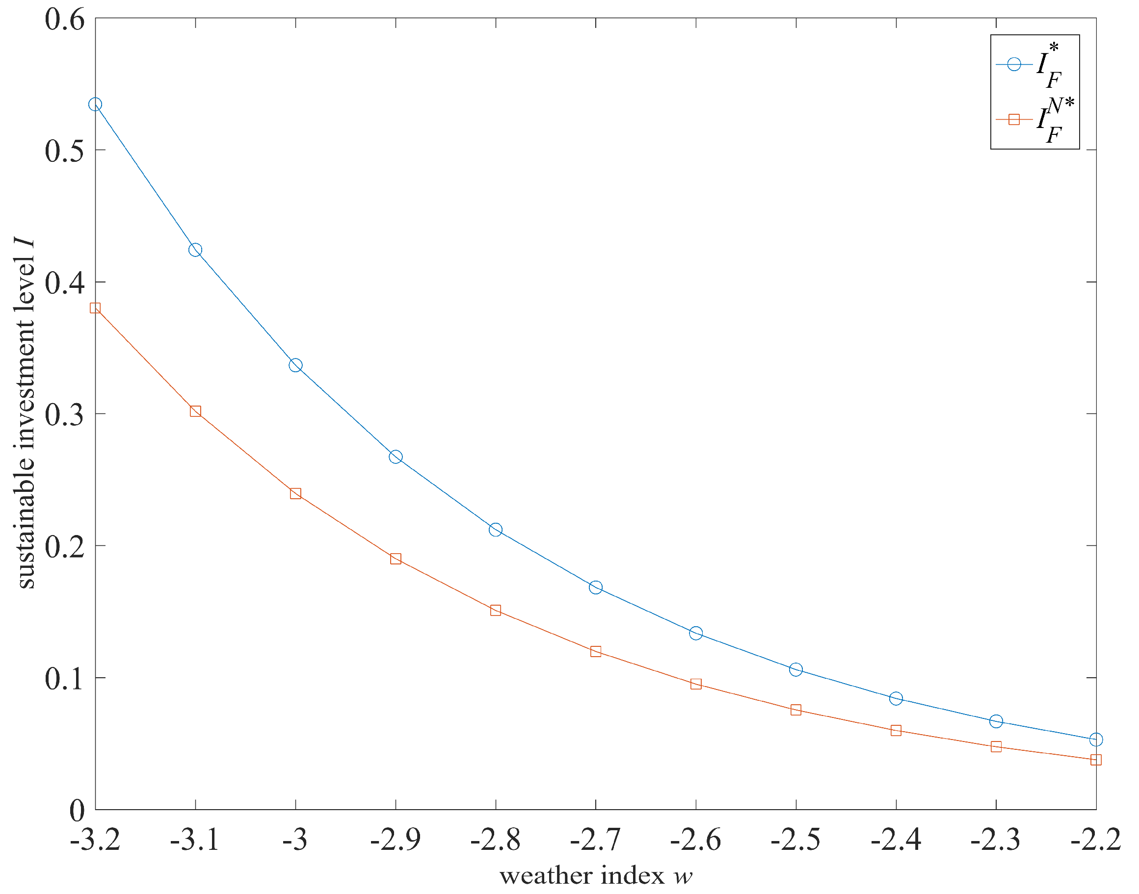
Proposition 3.

The implementation of the GPM can improve the farmers’ sustainable investment level. That is, $I_F^{N\ast }<I_F^{\ast }$ and $I_{F1}^{N\ast }<I_{F1}^{\ast }$ ($I_{F2}^{N\ast }<I_{F2}^{\ast }$) hold. Furthermore, the farmers’ sustainable investment level $I_F^{\ast }$, $I_{F1}^{\ast }$, and $I_{F2}^{\ast }$ are negatively correlated with respect to $w$, respectively.

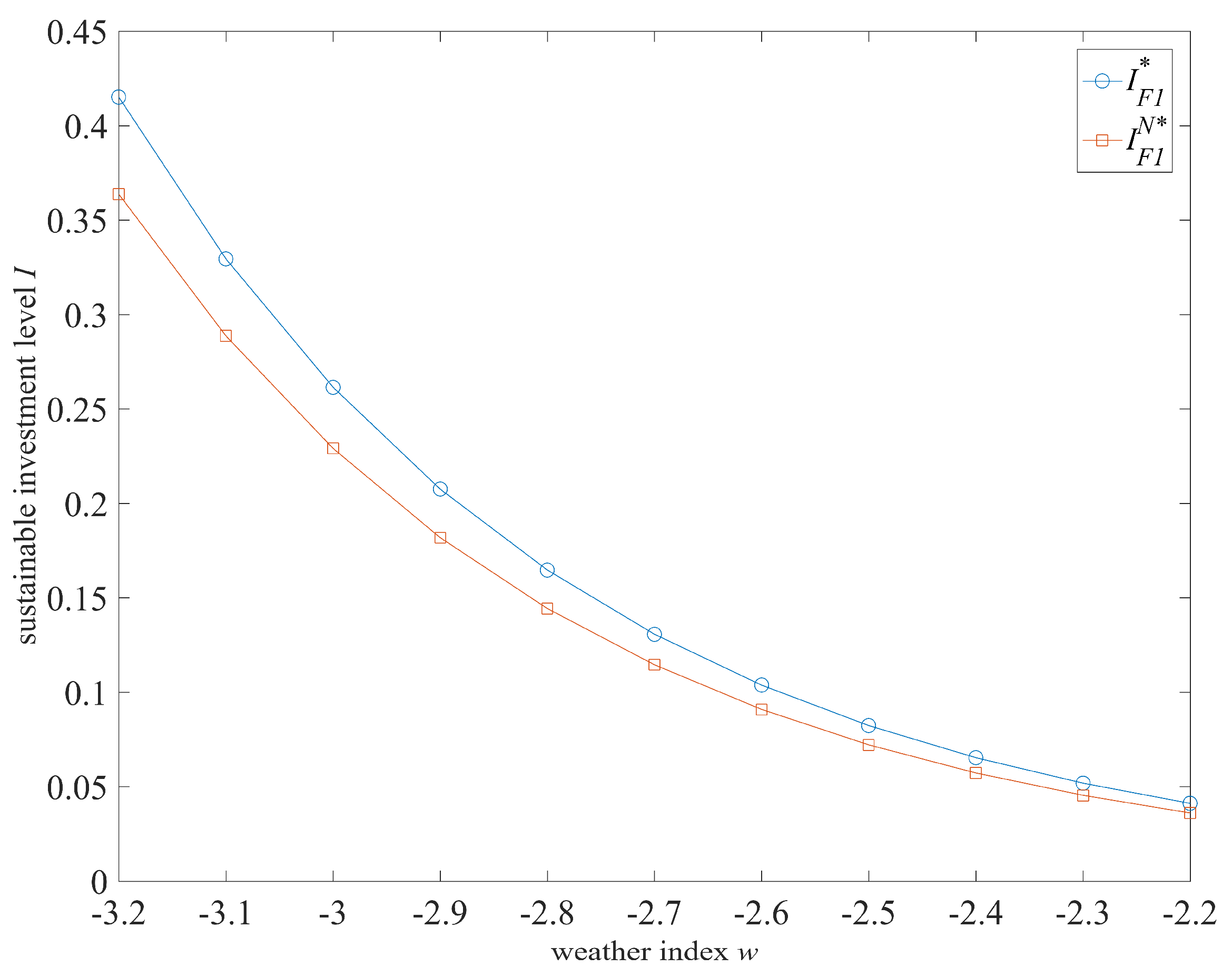
Figure 3 is a comparative analysis of the loss-neutral farmers’ optimal sustainable investment levels under the conditions of with and without the GPM; and Figure 4, taking the interval ${\omega }_{\min }\le {\omega }_C<{\omega }^{\ast }$ as an example, is a comparative analysis of the loss-averse farmers’ optimal sustainable investment levels under the conditions of with and without the GPM. Analysis shows that the implementation of the GPM can truly improve the sustainable investment level, which means that it is a practicable approach to inspire the farmer to enhance the sustainable investment level through the implementation of GPM such that the price risk faced by the farmer is shared. This on one hand checks the validity of Proposition 3. On the other hand, it shows that the implementation of the GPM can truly create value for sustainable agricultural practice. Moreover, Figure 3 and Figure 4 also demonstrate that the worse the adverse weather mild winter is (the value of w becomes larger), the lower the sustainable investment level is but the level tends to decline marginally. However, the loss-averse farmer is not only affected by the uncontrollable adverse weather, but also by his/her own loss preference in marketing decisions on the optimal sustainable investment level. Proposition 4 shows the relationship between the loss aversion coefficient and the sustainable investment level.

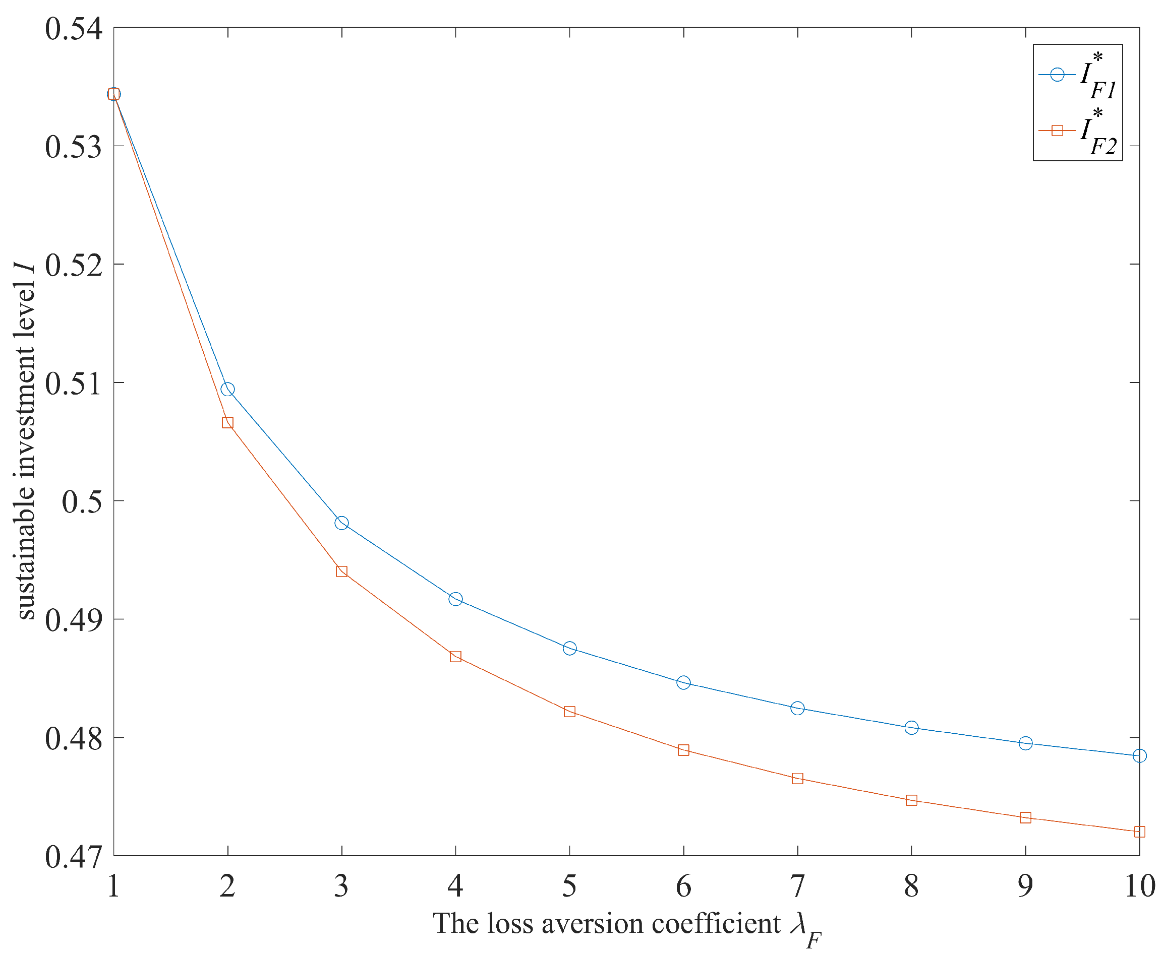
Proposition 4.

(i) Both $I_{F1}^{\ast }$ and $I_{F2}^{\ast }$ are monotonically decreasing functions with respect to ${\lambda }_F$, where ${\lambda }_F$ is in the interval $\left[1,+\infty \right)$. When ${\lambda }_F=1$, then $\max I_{F1}^{\ast }=\max I_{F2}^{\ast }=I_F^{\ast }$;

(ii) For any ${\lambda }_F$ such that ${\lambda }_F\ge 1$, it holds that $I_{F2}^{\ast }\le I_{F1}^{\ast }\le I_F^{\ast }<I_{SC}^{\ast }$.

We can make an in-depth analysis of Proposition 4, the results of which is shown in Figure 5. Whether or not it is under GPM, the sustainable investment level always declines when the farmers’ degree of loss aversion increases. That is, the farmer who is more averse to losses will pay a lower level of sustainable investment. The declining of the sustainable investment level not only leads to the decline of performance in the overall AFSC system, but also has a negative effect on the sustainable development of the agricultural practice environment. This inevitably will reduce the sustainability of the AFSC system. A further analysis of

Table 4. The optimal level of sustainable investment for given ${\lambda }_F=2$.

$\mathit{w}$	${\mathit{I}}_{\mathit{S}\mathit{C}}^{\ast }$	${\mathit{I}}_{\mathit{F}}^{\ast }$	${\mathit{I}}_{\mathit{F}1}^{\ast }$	${\mathit{I}}_{\mathit{F}2}^{\ast }$
−3.2	0.948146	0.534367	0.509411	0.506600
−3.1	0.755400	0.424128	0.404320	0.402089
−3.0	0.600992	0.336630	0.320909	0.319138
−2.9	0.477723	0.267184	0.254705	0.253300
−2.8	0.379528	0.212064	0.202160	0.201044
−2.7	0.301410	0.168315	0.160454	0.159569
−2.6	0.239319	0.133592	0.127353	0.126650
−2.5	0.189993	0.106032	0.101080	0.100522
−2.4	0.150820	0.084158	0.080227	0.079785
−2.3	0.119717	0.066796	0.063676	0.063325
−2.2	0.095025	0.053016	0.050540	0.050261

reveals that there is still a distortion of the sustainable investment level under the GPM, indicating that the GPM does not eliminate the effects of “double marginalization”.

Therefore, though the design of the GPM has positive influences, such as transferring the uncertain price risk faced by the farmer and improving the sustainable investment level, the existence of the “double marginalization” and the loss aversion preference of small households in developing economies will still reduce the sustainable investment level. This shows that there is still a need to further explore a contract mechanism between the company and the farmer.

5. Weather Risk–Reward: Improving Sustainable Investment Level

The design of GPM plays a positive role in encouraging the farmer to improve the sustainable investment level (Proposition 3). However, it fails to settle the adverse weather-led uncertain output risk and the decline of the sustainable investment level caused by the farmers’ loss aversion preference. The fundamental reason behind the failure is that the GPM does not take into account the influences of the adverse weather (like mild winter and cold spells in late spring) and the farmers’ loss aversion. To solve the distortion of the sustainable investment level caused by the “double marginalization” and to address the effects of uncontrollable adverse weather on the sustainable investment level, it is necessary to design a brand-new contract mechanism to improve the sustainable investment level, hedge the uncontrollable adverse weather risk faced by the farmer, and ensure a stable and sound operation of the SAFSC.

On the basis of the GPM, this section introduces a risk–reward contract by considering the weather index (taking temperature for example) and the farmers’ degree of loss aversion. Before the agricultural production season, the company and the farmer reach an agreement that the company will purchase the farmers’ produce at the price of $\tilde{\omega }=\max \left({\omega }_C,\omega \right)$ at the harvest season and will subsidize the farmer $\mathsf{\Upsilon }\left(w,{\lambda }_F\right)$ for unit quantity of produce to share the agricultural production risk faced by the farmer and encourage the farmer to improve the sustainable investment level in the agricultural practice. Under such weather risk–reward contract in the interval $\left(\tilde{\omega },\mathsf{\Upsilon }\left(w,{\lambda }_F\right)\right)$, the company’s expected profit is

$$E{\pi }_C^{wrr}\left({\omega }_C\right)=p\left(Q\left(I,w\right)-{\displaystyle {\int }_0^{Q\left(I,w\right)}G\left(x\right)}\mathrm{d}x\right)-\left(\mathsf{\Delta }\left({\omega }_{\max }\right)+\mathsf{\Upsilon }\left(w,{\lambda }_F\right)\right)Q\left(I,w\right)$$

(16)

The loss-neutral famer’s expected profit is

$$E{\pi }_F^{wrr}\left(I\right)=\left(\mathsf{\Delta }\left({\omega }_{\max }\right)+\mathsf{\Upsilon }\left(w,{\lambda }_F\right)\right)Q\left(I,w\right)-C\left(I\right)F\left({\omega }_{\max }\right)$$

(17)

When ${\omega }_{\min }\le {\omega }_C<{\omega }^{\ast }$, the loss-averse farmers’ expected utility is

$$E{U}_{F1}^{wrr}\left(I\right)=\left({\lambda }_F-1\right)\left[\left(\mathsf{\Delta }\left({\omega }^{\ast }\right)+\mathsf{\Upsilon }\left(w,{\lambda }_F\right)F\left({\omega }^{\ast }\right)\right)Q\left(I,w\right)-C\left(I\right)F\left({\omega }^{\ast }\right)\right]+E{\pi }_F^{wrr}\left(I\right)$$

(18)

When ${\omega }^{\ast }\le {\omega }_C\le {\omega }_{\max }$, the loss-averse farmers’ expected utility is

$$E{U}_{F2}^{wrr}\left(I\right)=\left({\lambda }_F-1\right)\left[\left({\omega }_{F}F\left({\omega }^{\ast }\right)+\mathsf{\Upsilon }\left(w,{\lambda }_F\right)F\left({\omega }^{\ast }\right)\right)Q\left(I,w\right)-C\left(I\right)F\left({\omega }^{\ast }\right)\right]+E{\pi }_F^{wrr}\left(I\right)$$

(19)

An analysis of Equations (18) and (19) shows that when ${\lambda }_F=1$, the loss-averse farmers’ expected utility is equal to the loss-neutral farmers’ expected profit, i.e., $E{U}_{F2}^{wrr}\left(I\right)=E{U}_{F1}^{wrr}\left(I\right)=E{\pi }_F^{wrr}\left(I\right)$. We now discuss the conditions for reaching the optimal sustainable investment level in the SAFSC among farmers with different loss preferences in Proposition 5.

Proposition 5.

Under the weather risk–reward contract $\left(\tilde{\omega },\mathsf{\Upsilon }\left(w,{\lambda }_F\right)\right)$, suppose that the risk–reward coefficient $\mathsf{\Upsilon }\left(w,{\lambda }_F\right)$ is such that

$$\mathsf{\Upsilon }\left(w,{\lambda }_F\right)=p\left(1-G\left(Q\left(I,w\right)\right)\right)-\left(\left({\lambda }_F-1\right)\mathsf{\Gamma }\left(s\right)+\mathsf{\Delta }\left({\omega }_{\max }\right)\right)/\mathsf{\Lambda }\left({\lambda }_F\right)$$

(20)

where $\mathsf{\Gamma }\left(s\right)=sF\left({\omega }^{\ast }\right)-{\displaystyle {\int }_{{\omega }_C}^{s}F\left(x\right)d}x$ (when ${\omega }_{\min }\le {\omega }_C<{\omega }^{\ast }$, $\mathrm{s}={\omega }^{\ast }$; when ${\omega }^{\ast }\le {\omega }_C\le {\omega }_{\max }$, $s={\omega }_F$). Then, the distortion of the sustainable investment level can be settled, namely $I_{F2}^{wrr\ast }=I_{F1}^{wrr\ast }=I_F^{wrr\ast }=I_{SC}^{\ast }$.

An analysis of Proposition 5 shows that an appropriate weather risk–reward coefficient will enable farmers with different loss preferences to reach the optimal sustainable investment level of the SAFSC system. Although this will increase farmers’ production cost, the company shares the farmers’ production risk by offering risk subsidies, which is beneficial to a stable supply of agricultural products and the sustainable development of the agricultural industry. Since the weather risk–reward contract overcomes the effects of “double marginalization”, stable and sound operations of the SAFSC system is guaranteed. Moreover, it is also found that the weather risk–reward coefficient is relevant to the degree of loss aversion and the weather index (temperature). A further analysis leads to Proposition 6.

Proposition 6.

(i) When ${\lambda }_F\ge 1$, an increased ${\lambda }_F$ leads to an increased $\mathsf{\Upsilon }\left(w,{\lambda }_F\right)$;

(ii) when $\underset{=}{w}\le w\le \underset{\_}{w}$, an increased $w$ leads to a decreased $\mathsf{\Upsilon }\left(w,{\lambda }_F\right)$;

(iii) when $\overline{w}\le w\le \stackrel{=}{w}$, an increased $w$ leads to an increased $\mathsf{\Upsilon }\left(w,{\lambda }_F\right)$.

On the basis of numerical examples, it is clear seen from Figure 6 that under the weather risk–reward contract $\left(\tilde{\omega },\mathsf{\Upsilon }\left(w,{\lambda }_F\right)\right)$, the reward coefficient is positively correlated with the farmers’ degree of loss aversion, meaning that the farmer who is more averse to losses will obtain a greater risk–reward. As such, this contract can encourage farmers to improve the sustainable investment level by increasing the amount of risk–reward. Furthermore, when such adverse weather, such as a mild winter (a higher temperature index means severer damages), appears, the weather risk–reward is positively correlated with the weather index. This means that severer adverse weathers lead to a greater risk–reward for the farmer. As such, this contract can encourage farmers to improve the sustainable investment level by improving the risk–reward to share the production risk faced by the farmer. When such adverse weather, such as a cold spell in late spring (a lower temperature index means severer damages), appears, the weather risk–reward is negatively correlated with the weather index. Corresponding numerical examples can be used for similar analysis.

Further analysis of Propositions 3, 5, and 6 reveals that the design of a GPM-based risk–reward contract $\left(\tilde{\omega },\mathsf{\Upsilon }\left(w,{\lambda }_F\right)\right)$ can improve the sustainable investment level, leading to the optimal sustainable investment level of the SAFSC system. This is beneficial to the stable and sound operation of the SAFSC. Under the weather risk–reward contract, the distortion of the sustainable investment level can be settled. But is it possible to make the company and the farmer reach their own Pareto performance? That is, when the company and the farmer make decisions on their own, they both have the motivation to fulfill the weather risk–reward contract. This requires further in-depth analysis.

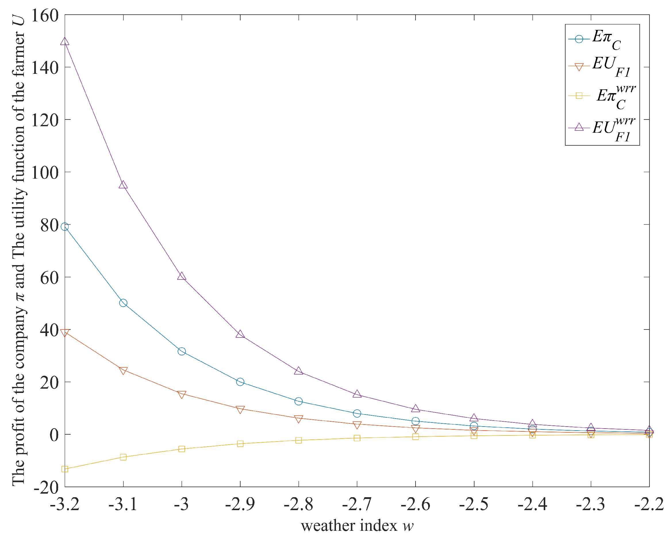
As shown in Figure 7, taking Situation 1 (${\omega }_{\min }\le {\omega }_C<{\omega }^{\ast }$) for example and under the condition that the farmers’ loss preference (${\lambda }_F=2$) is given, we make a comparative analysis of the company’s profit and of the farmers’ performance before and after the implementation of the weather risk–reward contract $\left(\tilde{\omega },\mathsf{\Upsilon }\left(w,{\lambda }_F\right)\right)$. It is found that after the implementation the farmer improves the performance while the company acquires less profit. This means that although the implementation of the weather risk–reward contract $\left(\tilde{\omega },\mathsf{\Upsilon }\left(w,{\lambda }_F\right)\right)$ overcomes the distortion of the sustainable investment level, it makes the farmer extract all the profit increased after the implementation of the contract. Consequently, the company would lack motivation to fulfill the contract but will have the motivation to foster further innovation. Therefore, before the production season, apart from the signing of the weather risk–reward contract, the company and the farmer need to agree with the design of a transferring payment mechanism ($T$). 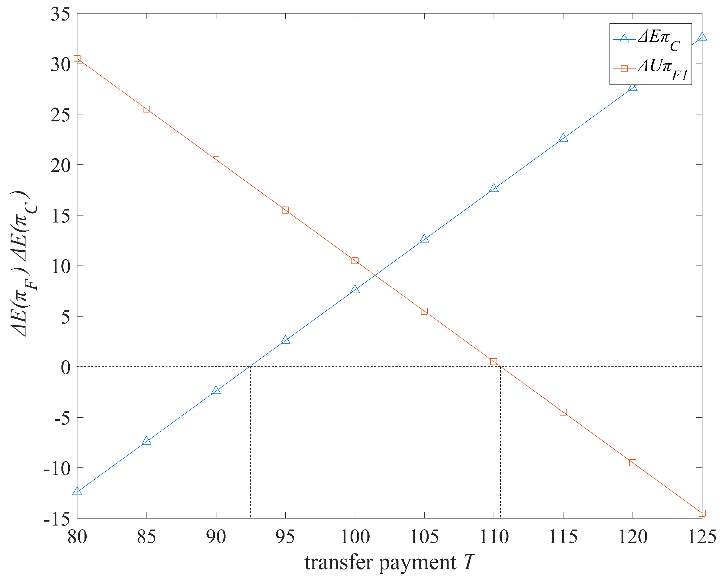Under this transferring design, when the farmer enjoys the right to the GPM and the risk–reward contract, he/she needs to provide the company with certain amount of transferred payment which can be regarded as the deposit for the farmers’ implementation of sustainable agricultural practice. The exact amount is to be negotiated by and between the farmer and the company. As shown in Figure 8, under the condition that the adverse weather index is given, the design of a rational transferring payment enables the SAFSC system to reach the optimal sustainable investment level and enables the company and the farmer to achieve a win-win situation. In this way, it guarantees the enforceability of the contract and is attractive to the sustainable and sound development of the AFSC.

6. Discussion and Conclusions

In this section, we respond to the questions introduced in Section 2 background and literature review. We have designed an effective contract mechanism, expecting to solve these problems and guarantee the sustainable production and operation of the AFSC in a better way. Moreover, we present the limitations and possible extensions of this study to overcome with further research based on the above analysis.

It is well known that the sustainable development of the AFSC will inevitably encounter such problems as unfair pricing, uncertain output caused by adverse weather (such as mild winters, cold spells in late spring, drought, and heavy rain), as well as conflict and coordination between AFSC stakeholders. We made an analysis of the two-echelon SAFSC system consisting of one loss-averse farmer and one loss-neutral company, and proposed the GPM for mitigating the influence of unfair pricing on the farmers’ profit. We found that the design of guaranteed price can protect farmers’ profit in the uncertain environment on product prices. From Proposition 3, we know that GPM can improve the farmers’ sustainable investment level, which means that the company should offer the price protection contract to the farmer in agricultural production practices. In order to further address the conflict and coordination between these two parties under the influence of adverse weather and loss-averse preference, we contrived a GPM-based weather risk–reward contract by taking into account the weather index (temperature) and the degree of loss aversion, and studied the value of this contract to the SAFSC. From Proposition 5, we know that a weather risk–reward contract can hedge the adverse weather risk and guarantee increased benefits for farmers so as to improve the sustainable investment level, which means that the company should offer a GPM-based weather risk–reward contract to the farmer in order to achieve a win-win situation and reach the optimal sustainable investment level in the SAFSC system.

The paper has found several helpful managerial insights and interesting observations in the practice of SAFSC. First, although the design of the GPM can, to some extent, mitigate negative effects of unfair pricing on the farmers’ profits, it may, at the same time, breed farmers’ opportunist behavior in sustainable agricultural practices. Hence, we acquire a counterintuitive observation: it is not always better for the farmer when the guaranteed priced decided by the company is higher. When the guaranteed price exceeds the point of balance between profit and losses, an increase of the guaranteed price will not result in an increase of the farmers’ expected utility. Second, the implementation of the GPM can, to some extent, effectively improve the sustainable investment level, meaning that the design of the GPM can truly create value for the sustainable agricultural practice. However, the GPM fails to settle the distortion of the sustainable investment level. The fundamental reason behind such failure is that the GPM does not take into account the influence of the exogenous adverse weather on agricultural production and the loss preferences of the farmer who acts as the executor of the sustainable agricultural practice. Therefore, there is still a need for further investigation. Third, a GPM-based risk–reward mechanism, which takes into account the weather index and the degree of loss aversion, was contrived. An appropriately chosen weather risk–reward coefficient can solve the distortion of the sustainable investment level. That is, farmers with different loss preferences can fulfill the optimal sustainable investment level of the SAFSC system, which is beneficial to a stable and sound development of the SAFSC system.

There are several limitations and insufficiencies in the paper. First, this paper studies the uncertainty of agricultural output under the influence of adverse weather (such as mild winter, cold spell in late spring, drought, and heavy rain). However, from the perspective of global supply chains, the supply of agricultural products also encounters the problem of uneven distribution of agricultural products. How to match the supply of agricultural products with their demand in a fair and rational way is a meaningful topic for further research. Second, we study the design of weather risk–reward contract in SAFSC to achieve a win-win situation. However, we do not provide metrics of performance of company, farmer, and ‘other’ stakeholders. Third, we do not analyze the value of social responsibility of the company, but many studies do it [20]. Consequently, the value of company’s social responsibility in SAFSC will be an interesting research issue in the future. Last but not least, this paper uses the sustainable investment level to quantitatively represent the sustainable agricultural practice. This kind of representation needs further research, such as, how to quantify the social and environment responsibilities of the AFSC in its sustainable operation, how to design a sustainable contract mechanism to motivate AFSC stakeholders to participate in the sustainable development, etc.