Article

Flooding in Central Chile: Implications of Tides and Sea Level Increase in the 21st Century

1
Department of Territorial Planning, Faculty of Environmental Sciences and EULA Chile Center, Universidad de Concepcion, Concepción 4089100, Chile
2
School of History, Geography and Political Science, Institute of Geography, Pontificia Universidad Católica de Chile, Santiago 7820436, Chile
3
E.O.H. Engineer, Viña del Mar 2520000, Chile
4
Department of Statistics, Faculty of Mathematical and Statistical Sciences, Universidad de Concepcion, Concepción 4089100, Chile
5
Department of Aquatic Systems and EULA Center, Faculty of Environmental Sciences, Universidad de Concepcion, Concepción 4089100, Chile
*
Author to whom correspondence should be addressed.
Sustainability 2018, 10(12), 4335; https://doi.org/10.3390/su10124335
Submission received: 1 October 2018 / Revised: 15 November 2018 / Accepted: 16 November 2018 / Published: 22 November 2018
(This article belongs to the Special Issue Floods and Landslides: A Sustainability Approach)

Abstract

:
Coastal floods have become a serious problem on a global scale, increasing in frequency or magnitude due to natural conditions, and exacerbated by socioeconomic factors. This investigation analyzes the role of tides and average sea levels on the development and intensity of flooding in the lower section of the Andalién River, located toward the southern extreme of the coast of central Chile and northeast of Concepción, the country’s second most populous city. Numerical simulation (1D) was used in five modeled scenarios to determine potential flooding areas, demonstrating the influence of tides in flooding processes as far away as 7.3 km from the river mouth, which is reinforced by the fact that 57% of flooding events occur during syzygies. Further, a climate change-induced sea level rise of 60 cm from current levels by the end of the 21st century would produce a 4% increase in flood-prone areas, with 17% of flooding affecting the current built-up area and 83% of floodplains and salt marshes. Efforts must be made to protect or conserve these latter areas in order to increase natural resilience, given the high costs of implementing structural measures to protect future residential areas.

1. Introduction

Currently, the need for society to adapt in the face of natural hazard scenarios heightened by natural and socioeconomic factors is emphasized [1]. In this regard, coastal floods have become a serious problem on a global scale [2,3]. Close to 50% of the global population is concentrated in coastal areas, which are densely populated and economically attractive [4,5,6]. In the 20th century, the frequency of floods and the magnitude of damages increased [7], and a significant further increase in flooding risk is expected in the 21st century, according to models of average sea level rise (ASLR) due to global climate change (GCC), land-use changes driven by global socioeconomic growth [4,8,9,10,11], and population growth [12].
Floods in Mediterranean coastal basins are generally caused by intense precipitation [13,14]. When rivers form mixed estuaries in plains with low channel slopes, tides can become a key factor for flood generation [5,6,15]. The tide forms a boundary condition downstream in the estuary, which, synchronized with high discharges resulting from high amounts of precipitation, impedes the discharge of water, increasing the risk of flooding [4,16,17]. Extremely high tides are caused when astronomical, meteorological, and climatic factors coincide [11,18,19]. Phenomena related to astronomical factors are quadrature and syzygies tides, the latter of which have the highest tide levels. Rojas and Mardones [20] established an 80% correlation between floods and syzygy tides in the Valdivia River estuary (39° S, Chile). In addition, high winds and low atmospheric pressure due to storms can produce large swells, known as meteorological tides [15], which, when combined with climatic conditions like the El Niño–Southern Oscillation, are capable of increasing the average sea level by 0.1–0.3 m [11].
Tide levels and storm surges will be affected by GCC [21]. Global climate models predict a sea level rise of between 0.26–0.85 m, with a high level of regional variability [4,19,22,23]. Historically, sea levels have fluctuated in Chile, with rates of increase of up to 0.32 cm/year and rates of decrease of −0.14 cm/year [24]. Concepción Bay (36° S) underwent a sea level rise of 88 mm over 59 years (1949–2008), expressed as an annual increase of 1.5 mm/year [24]. A previous study of the same bay established an average sea level of 1.10 m between 1949–1994, with a progressive increase starting in 1974 [25]. The IPCC [23] estimates that by the year 2100, Chile will have experienced a SLR of between 0.3 in the best-case scenario (model RCP 2.6) and 0.6 m in the worst-case scenario (model RCP 8.5).
Chile has been identified as a country at risk of an increase in storms and floods [13,26], owing to its geographical characteristics, the variety of climatic zones, mountainous terrain, environmental changes, and populated river plains [13,14,27]. During the period of 1900–2012, 57 flooding events were recorded in the Mediterranean zone of Chile, where 73% of the national population is located [28]. The population is concentrated in the metropolitan area of Santiago, and in the coastal cities of Valparaiso and Concepción (AMC in Spanish).
The Andalién River (36° S), the lower section of which discharges into Concepción Bay, is located in the AMC. This region experienced a 700% increase in urbanized area between 1955–2007 [29]. There were 21 flooding events between 1960–2010, and five of the high magnitudes between 2000–2010 [14]. According to the Regional Emergency Office (OREMI), the 2005 disaster caused upwards of US$6.5 million in damages [30]. Although flooding in the area has been studied [14,30,31,32,33,34,35,36], there is a lack of knowledge surrounding the role of tides and potential SLR. Understanding these factors is a priority in land-use planning associated with adapting to GCC [37,38,39].
The Andalién River forms a mixed estuary. Therefore, it has been proposed that historic flooding events with important environmental effects are significantly correlated with syzygies and potential SLR attributed to GCC. This study examines the effects of historical tide levels and potential SLR due to GCC in Concepción Bay on river floods in the lower section of the basin. To this end, we completed (1) a physical characterization of the lower section of the basin, in order to categorize its environments as lower, middle and upper zones and (2) a numerical simulation (1D) of a high-magnitude flood, which includes five modelled scenarios with different boundary conditions (astronomical and meteorological tides and a projection of sea level rise). In addition, we determined which geomorphological and urban zones of the region are at risk of flooding.

2. Materials and Methods
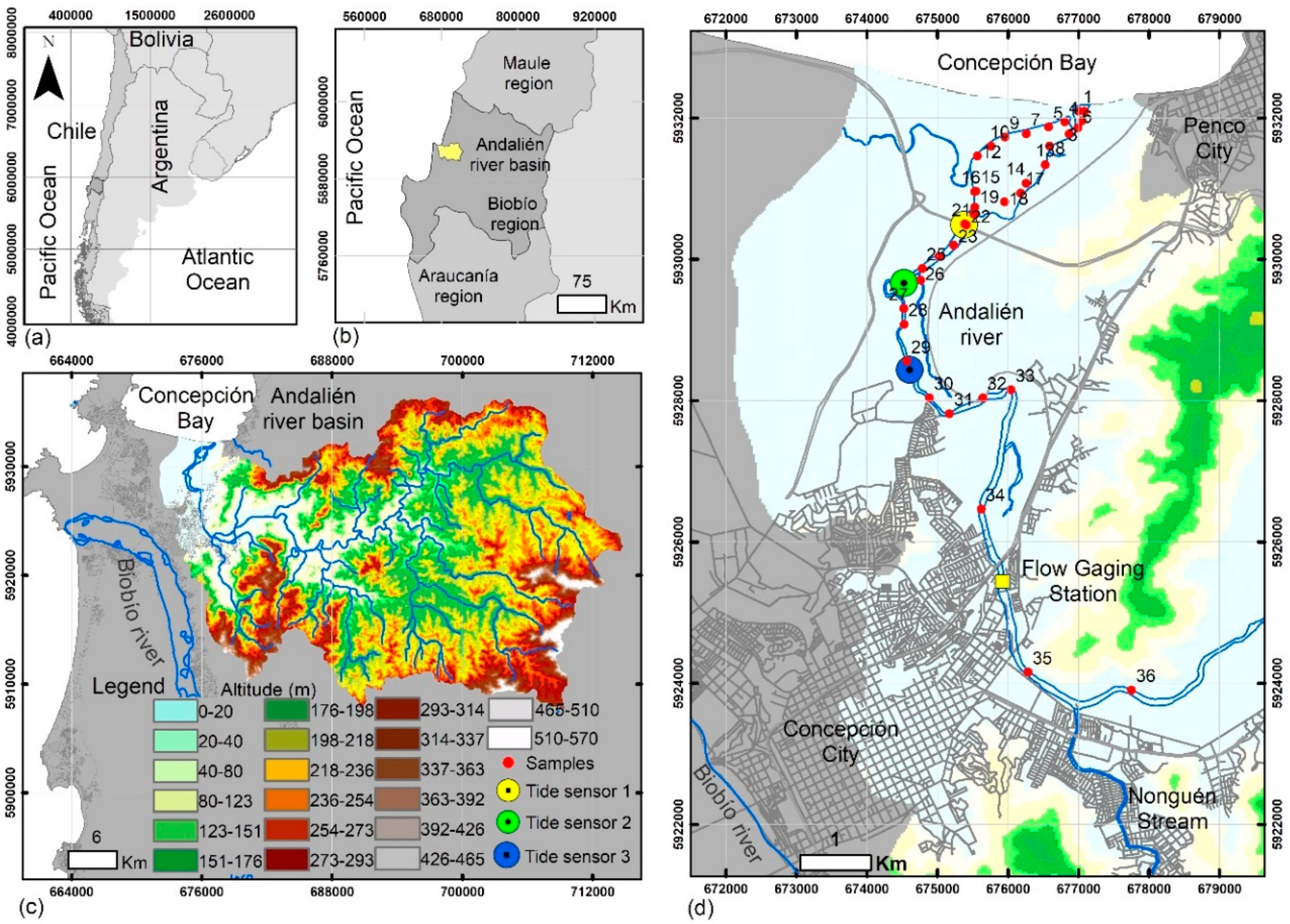
2.1. Study Area

The Andalién River basin (715 km2) is part of the Coastal Range (36° S), and it is located in the Biobío region of Chile. Geomorphologically, it is predominantly (60%) mountainous. Granite platforms make up 20% of the basin, while the terraces and plains of the lower section of the river, on which part of the city of Concepción was built, account for 4% (Figure 1) [40]. In 2002, the city was inhabited by an estimated 90,000 people. The population has been increasing at a sustained rate for the last three decades, and has reached a density of 15,000 individuals/km2 [41].
The area has a Mediterranean climate, with an annual precipitation that fluctuates between 1200 and 1600 mm annually in the western and eastern regions of the basin, respectively [42]. In the austral winter, five-day episodes of continuous rain are common, with rainfalls of up to 124 mm/24 h [40,43]. At the lower end of the basin, the river’s mean annual flow reaches 14 m3/s. Winter floods can be destructive; at T = 50 and T = 100 years, instantaneous discharges of up to 565 m3/s and 634 m3/s are estimated [44].
Before the river discharges into Concepción Bay, it transforms into an estuary in the NE quadrant of the basin, which stretches from the outlet three kilometers up the primary river channel. The estuary itself has the following features: from 0–1 km, the primary riverbed is singular and semi-rectilinear, with unstable processes on the sand spit and estuary bars caused by runoff during floods; from 1.1–3 km, the river splits into a delta-like formation with various secondary riverbeds and the central bank of the estuary exhibits accretion processes (1–1.8 km); between 3.4–4.1 km, obstruction caused by runoff from sediment banks can be observed [45].

2.2. Methodology

2.2.1. Physical Characterization of the Lower Section of the Basin

A physical characterization of the lower section of the basin was completed to establish different environmental zones (lower zone, middle zone, upper zone) in order to determine the maximum intrusion of salinity into the system, and to validate the results that are obtained in the applied hydraulic model. Conglomerate analysis was used to characterize each environment. We carried out a one-way analysis of variance (ANOVA) and applied the Tukey test (α = 0.05) to compare different zones (estuarine, middle, upper).
Sampling of physical–chemical variables in spring and winter conditions was undertaken on 21 November 2013, and 25 August 2014, respectively. Both samples were taken during syzygies and during complete tidal cycles [46]. Temperature (°C) and salinity (psu) data were collected in both shallow and deep water at nine stations during winter sampling, and 36 stations during spring sampling (Figure 1), with the goal of detecting tidal salinity. The station locations were established via dual-frequency GPS, and station depth was obtained with a digital echo-sounder installed on the boat. The standard ecological coastal–marine classification system proposed by Madden et al. [47] was used to classify the physical–chemical variables.
At each station, surface sediment samples were collected with a manual dredge. The samples were sifted to a particle size of 4.0 Φ. The small particles were analyzed with the Elzone 282 PC Coulter Counter (Laboratory Sedimentology, EULA Center), while the large particles were analyzed via sieves (Laboratory of Physical Geography, FAUG). We used Wentworth’s [48] classification and the Folk et al. [49] ternary triangle to establish the grain size. GRADISTAT software was used to integrate data from the coarse and fine grain samples [50].
Three HOBO (model U20) tide sensors (Figure 1) were installed to detect monthly syzygies and to determine the influence of dynamic tides on the estuary under spring conditions. The sensors operate continuously for a period of 15–30 days and have a recording interval of 5 min. For winter conditions, this information was obtained through salinity data from winter sampling.
The estuary was classified according to Davies’ [51] tidal ranges. To quantify the degree of stratification in the estuarine channel, we applied the mixed parameter ( n s ) [52] to each of the sampling stations during both spring and winter samplings. n s is defined as:
n s = δ S S m
where δ S = S p r o f S s u p ,   S m = 0.5 ( S p r o f + S s u p ) , and S p r o f and S s u p correspond to salinity in deep and shallow segments of the water column, respectively. If n s < 0.1 , the water column is completely mixed, when 0.1 < n s < 1.0 , it is partially mixed, and when n s > 1.0 , the column is stratified with an evident saline wedge.

2.2.2. Hydraulic Modeling and Sea Level

A historical analysis of the relative magnitude of the floods that occurred between 1960 and 2010 [53] and the astronomical tide (AT) and meteorological tide (MT) records obtained from the tide tables and tide gauge of the port of Talcahuano (36°41′43″ S, 73°06′22″ O) was carried out. This information was provided by the National Center of Hydrographic and Oceanographic Data of the Hydrographic and Oceanographic Service of the Chilean Navy (CENDHOC-SHOA). We calculated the residues (Residues = MT − AT) that correspond to each flood magnitude. The lunar phase data used to categorize the tides as syzygies and quadrature tides were obtained from the U.S. Naval Observatory.
As a secondary step, Hec-Ras 4.1 software was used to carry out (1D) hydraulic modeling [54]. The astronomical tide was evaluated under both quadrature and syzygy conditions. In addition, we considered scenarios including meteorological factors and conditions due to extreme SLR caused by GCC. The choice of GCC models used in this study is consistent with the recent IPCC report [23] and Kopp et al. [55]. For flow data, we used an extreme discharge (Dmax) with a return period of 100 years (exceedance probability 1 p 0.01 ) [44].
The meteorological and astronomical tide level data ( S L R 0 ) for the five scenarios were obtained from the CENDHOC-SHOA. We obtained data for the 1961–2006 period for days when flooding events occurred, according to Rojas [53]. The contribution of sea level rise ( Δ S L R ) was calculated using the RCP2.6 scenario as the low extreme and the RCP8.5 scenario as the high extreme. Total tide heights ( Δ H t = S L R 0 + Δ S L R ) (Table 1) for five SLR scenarios were entered into the software as flow boundary conditions.
A topo-bathymetric data was used to obtain the geometric data in the hydraulic model. Two LIDAR (Light Detection and Ranging) flights were conducted, the first of which had a resolution of 2.5 m (Maritime Port Research Centre; CIMP in Spanish), and the second, of the zone directly around the river channel, had a resolution of 1 m. Due to the difficulty of penetrating the surface of the water with LIDAR, the bathymetry was constructed using two different data sets. From the mouth of the river to km 4, the GARMIN echo sounder model FF400C was used, the transducer of which was mounted on the side of a fishing boat and supported by a TRIMBLE R-4 dual-frequency GPS, and linked to geodetic points. From 4–12 km, considering the low depth, a correction of the riverbed was performed for the slope criteria, as established by Arrau Igeniería E.I.R.L. [44]. The selected coordinate system was WGS_1984_UTM_Zone 18 S; altitude data was relative to the mean sea level (MSL).
The HECgeo-RAS 4.3.1 in ArcGIS 9.3 (3D Analyst Toolset) was used to generate the data profiles [56]. This information permitted 206 cross sections with variable equidistances of between 50–100 m to be obtained for 12.8 km of THE river channel. Manning’s roughness coefficient (n) [57] was applied to the channel and floodplain sections of each cross section, obtained through observation and photos that were georeferenced in the field. The coefficient was calibrated using the work of Inostroza [34], as well as a sensitivity analysis of ±10% of the assumed value, under conditions that were obtained in the field during the spring of 2014, with a discharge of 36 m3/s and a boundary condition of 1.5 m.
Using the results of our numeric modeling, five flood maps were constructed with SIG ArcGIS 9.3 [56]. The results were cross-referenced against the geomorphological zones and urban surface area established by Rojas et al. [14] for 2011, which were kept constant (U0).

3. Results

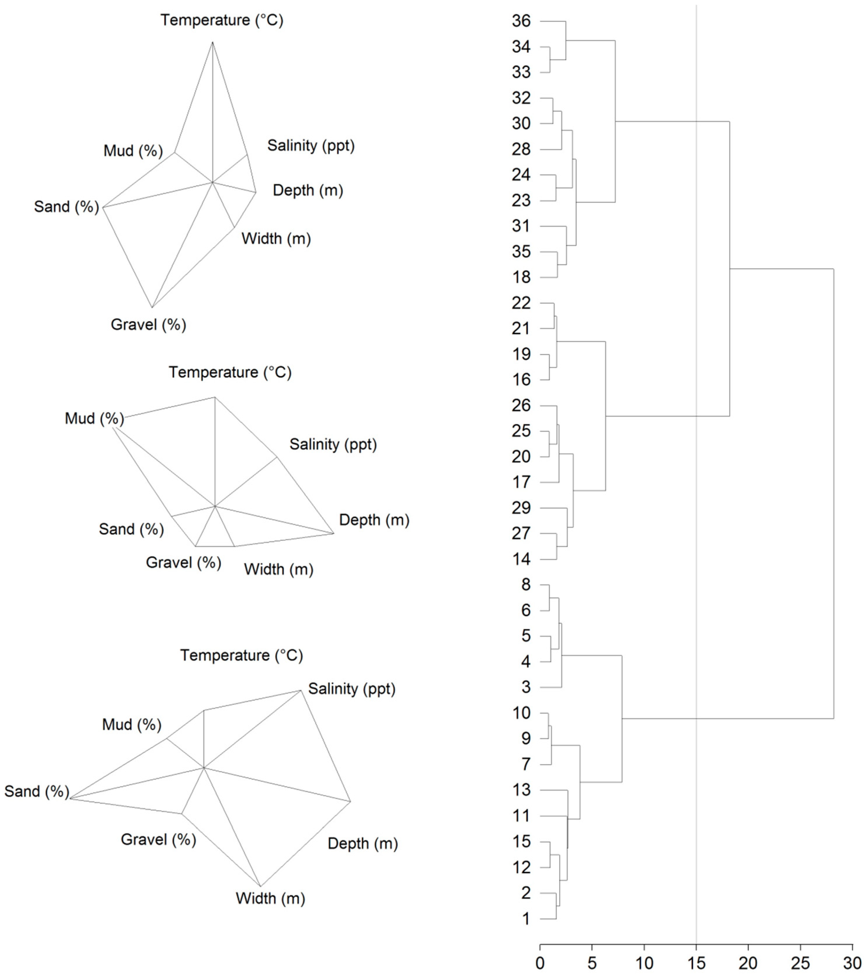
3.1. Physical Characterization of the Lower Section

The lower section of the Andalién River (0–15 km) can be divided into three main environmental zones according to the following variables: salinity, temperature, riverbed width and depth, and textural sediment distribution (Figure 2). The zones are: the lower estuarine zone (mouth to 2 km), middle estuarine zone (2–6 km) and the upper estuarine zone (km 6 to upper valley).
The ANOVA analysis showed significant differences between the three environments (p < 0.05) (Table 2). The temperature gradually increased from the lower zone (Cluster 1) to the upper zone (Cluster 3) (+7.7 °C), while the salinity decreased by 21.38 psu. The depth of the upper zone was approximately 0.7 m, compared to >1 m in the lower zone. The river channel was widest in the lower zone (157 m), while its width in the middle and upper zones was approximately 65 m. With respect to the granulometry, the gravel percentage was higher in the upper zone (16.9%), and the sand percentage varied heavily between zones. The lower (85.4%) and upper (69%) zones were predominantly sandy, while the middle zone had a much higher percentage of mud (66.2%).

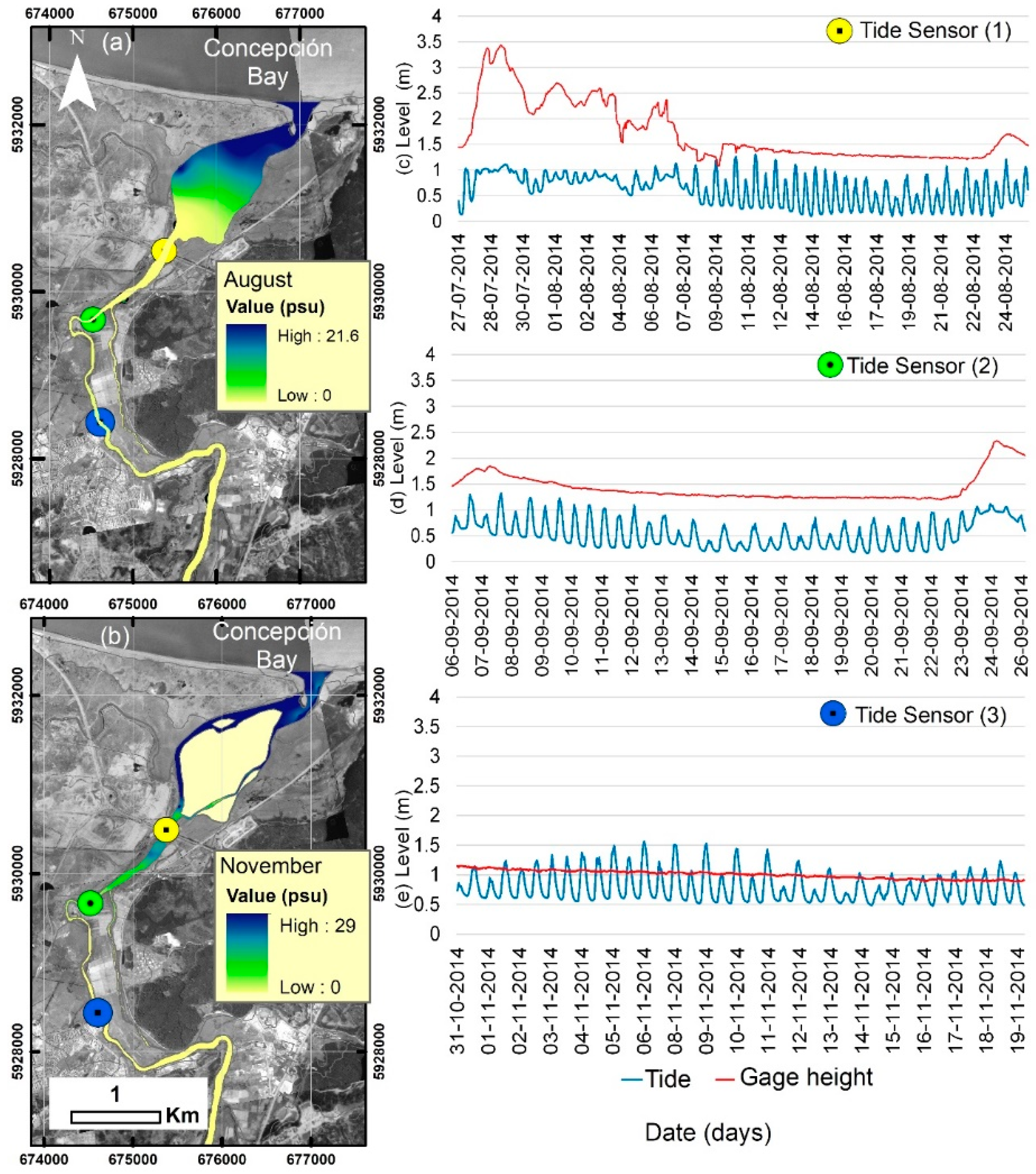
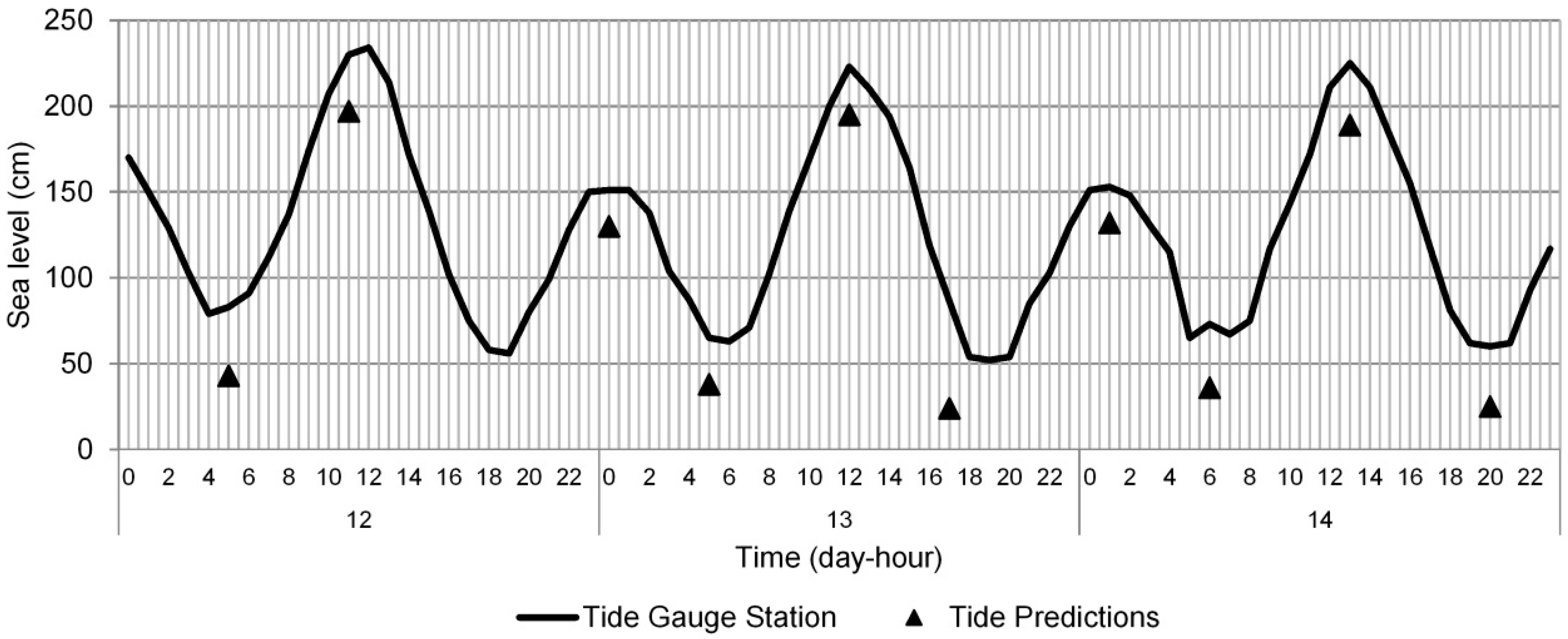
3.2. Tidal Inflow into the Estuary and River System

The Andalién River estuary can be defined as a partially mixed, microtidal estuary (tidal range < 2 m). The greatest intrusion of dynamic tides into the estuary takes place in the spring. Dynamic tides can reach 5.9 km upriver from the mouth, while salinity can only be detected up to 3 km. Maximum tidal amplitudes occur during syzygies. Tidal amplitude progressively decreased from the mouth to the estuary, and it was affected by increased river flow rates caused by precipitation.
The greatest tidal amplitude was recorded by Sensor 1, located in the middle zone of the estuary 2.5 km upriver from the mouth. On 14 July 2014, an amplitude of 1.45 m was recorded (Table 3); the Talcahuano tide gauge recorded a maximum amplitude of 1.6 m on the same day. The sinusoidal character of the tide was heavily affected by a precipitation-induced, increased river flow rate. Figure 3c shows that tidal waves were recorded beginning from 8 August, when the flow rate dropped from 208 m3/s (its 29 July rate) to <60 m3/s.
Sensor 2, located 3.5 km from the mouth, recorded a maximum amplitude of 0.81 m on 7 September (Table 3). On the same day, the Talcahuano tide gauge recorded an amplitude of 1.66 m. When the river flow rate stayed below 40 m3/s, the tidal wave was clear. When the flow rate fluctuated between 40–65 m3/s, the tidal range diminished substantially (Figure 3d). The greatest tidal penetration was recorded by Sensor 3 (Figure 3e), located 5.9 km up the estuary from the mouth. The value oscillated between a maximum of 1.57 m and a minimum of 0.48 m. A maximum amplitude of 0.94 m was recorded on 6 November. On the same day, the Talcahuano tide gauge in the bay recorded an amplitude of 1.64 m, and the river flow rate fluctuated between 11 m3/s and 3 m3/s.
The Andalién estuary behaved as a partially mixed estuary in terms of salinity; during the spring and winter, surface salinity was always less than the bottom salinity. During winter sampling, with a flow rate of 28 m3/s, the tidal influence on salinity was recorded up to the lower estuarine zone (1.78 km) (Figure 3a). The bottom salinity fluctuated between 16.6–21.7 psu, while the surface salinity fluctuated between 1.6–13.6 psu across all sampling stations (1–26). The highest salinity value (29 psu) was recorded in the bottom stations of the lower estuarine zone (station 10). The stratification parameter was 0.9, which is indicative of partial mixing.

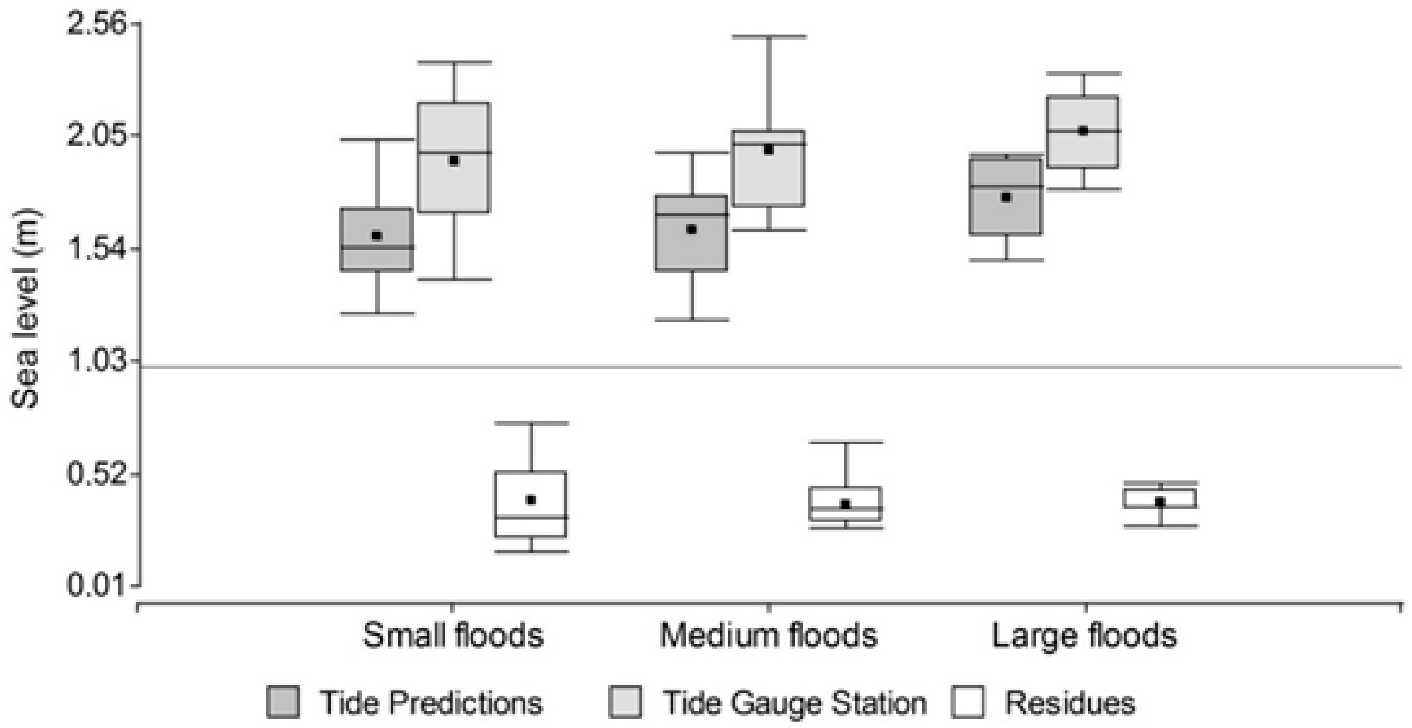
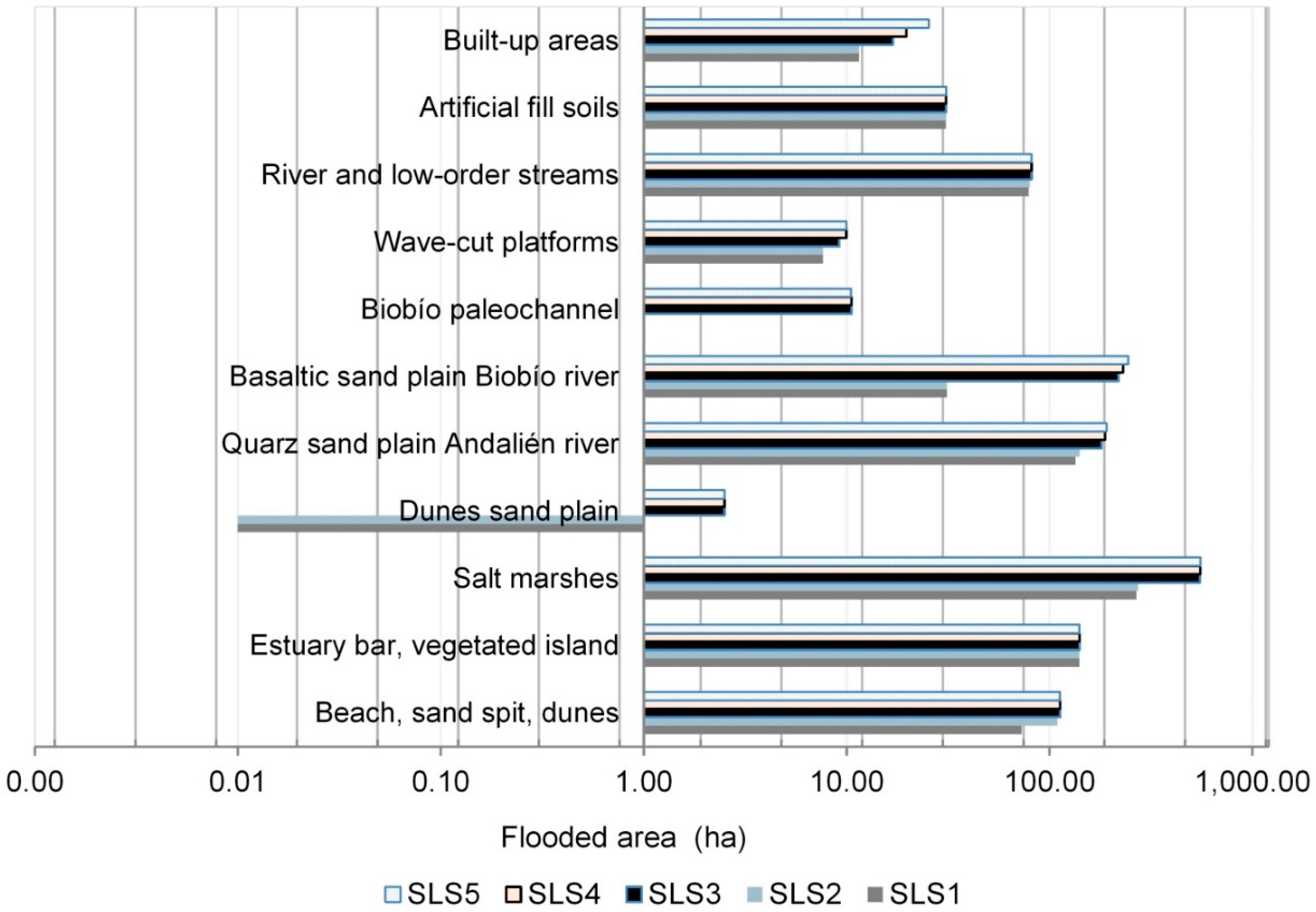
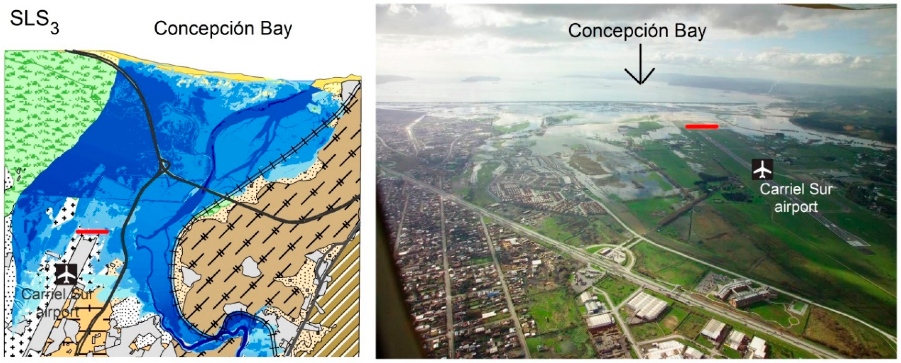
3.3. Tides and Floods

Historical astronomical tide records indicate that 57% of floods have occurred during or adjacent to syzygies, and 33% have occurred during quadrature tides. The maximum quadrature tides reached 1.8 m due to meteorological conditions, similar to the predicted values during syzygies. The mean high tide value during astronomical tides on flooding days was 1.63 m (S.D. 0.23). Meteorological tides raised the mean high tide level to 1.98 m (S.D. 0.27). Residues were found an average of +0.39 m above the predicted height.
In terms of relative flood magnitude, in small, medium, and large floods, the maximum average predicted tides were 1.63 m (S.D 0.21), 1.59 m (S.D. 0.24), and 1.78 m (S.D. 0.20), respectively. For small, medium, and large floods, the tidal gauge records showed 2.02 m (S.D. 0.24), 1.92 m (S.D. 0.31), and 2.08 m (S.D. 0.19), respectively. Residues were observed around 0.40 m, although with greater variability in small and medium floods, (S.D. 0.16 and S.D. 0.19, respectively); large floods had less variability (S.D. 0.07) (Figure 4). For example, during the large-magnitude flood of 2006, values from the tide gauge records were greater than the predicted values by 16% and 99% for the high and low tide, respectively (Figure 5). On 12 July, the maximum tide level was 2.30 meters, while the maximum predicted level was 1.97 m. The average high tide residues during the flood were at 0.27 m, while the average low tide residues were at 0.40 m.
In terms of hydraulic modeling, with a D100 and different sea level scenarios, the tidal influence on flooding in the worst-case scenario was observed up to 7.3 km from the mouth. Due to the astronomical conditions in SLS1 and SLS2, the tide played a smaller role in the flooding event. In SLS1, which modeled a low quadrature tide, the tidal influence on the flood reached 5 km. In SLS2, which modeled a syzygy with no meteorological factors, the influence of the tide reached the upper border of the middle zone (6 km).
In scenario SLS3, in which syzygy conditions and meteorological tides were considered, the influence of the flooding reached the lower limit of the upper section (7 km). In the climate change scenarios SLS4 and SLS5, in which an increase of between 30–60 cm of the maximum tidal value was considered, the flooding influence reached up to 7.3 km, where the average slope of the riverbed increases to 0.8 per thousand (8–14.9 km). From 7.3–14.9 km, the influence of the tide was not observed.
The most important change in the five scenarios analyzed was related to the surfaces affected by the flood. The greatest impact was observed in geomorphological units with low slopes (0.5°) and elevations <3 msl. In scenarios SLS1 and SLS2, the floods advanced steadily from the northern limit of the marine erosion platform located to the west of the riverbed toward the mouth. However, the presence of the Interportuaria Highway and railway lines, both of which run along a north–south axis parallel to the river bed, acted as a barrier that prevented the flood from advancing further, as they are built on an elevated dyke that is approximately +2 m high (Figure 6).
In SLS3, the increased water level, due to meteorological conditions, caused the flooding of the northwest section of the Interportuaria Highway and the northeast section of the railway lines, both of which are located close to the mouth. The flooding was propagated by the salt marsh, due to the low-lying nature of the area (0.1 msl). In the climate change scenarios SLS4 and SLS5, the flooding exceeded the heights of the Interportuaria Highway and railway lines near the river mouth and east of Carriel Sur Airport. The maximum water depth fluctuated between 2–3 m over the Rocuant-Andalien marsh, and between 1.5 and 2 m in the artificial-fill zones to the east of the airport. The velocity of the advancing flow stayed below 0.7 m/s.
With respect to the surface area of the flooding, SLS1 covered 774 ha and SLS2 covered 825 ha, in part due to the astronomical conditions of these models. In terms of the composition of the flooded area, 72% was sandy beach, sand spit, and dunes, 12% salt marshes, and 13.8% sand plains of the Andalién River (Figure 7). The meteorological conditions evaluated in SLS3 expanded the flooded area to 1352 ha, of which 52% comprised salt marshes, 35% floodplains formed by basaltic sand from the Biobío River, and 7.3% floodplains of the Andalién River. This last simulation condition produced a flood similar to that of June 2006, which similarly did not affect Carriel Sur Airport (Figure 8).
Potential increases of 30 cm (SLS4) and 60 cm (SLS5) in average sea level due to climate change by the end on the 21st century would expand the flood area by an additional 25 ha and 50 ha, respectively, in comparison with the current worst-case scenario, SLS3. The most heavily affected areas would be the basaltic sand plain of the Biobío River, (49.5%), the quartz sand plain of the Andalién River (21.1%), salt marshes (10.6%), and built-up areas (17%). The primary urban zones which would be affected are the Interportuaria Highway and the railway lines, but the artificial-fill zones that are currently being developed and, according to our results, are in a flood-prone area, should also be considered.

4. Discussion

The Andalién River forms a microtidal estuary with average tidal ranges of <2 m. By comparing historical flooding records and tidal levels, we determined that 57% of floods occurred near or during syzygies. In Southern Chile, Rojas and Mardones [20] established that in the microtidal estuary of the Valdivia River (39° S, Chile), 80% of floods occurred during syzygies. According to Garcés-Vargas et al. [58], in winter, this estuary behaved as a salt wedge, with depths of between 7–22 m and a tidal influence reaching 50 km upriver from the mouth. In comparison, in winter, the Andalién River behaved as a highly stratified mixed estuary, with a depth of between 0.5–2.5 m, and a tidal intrusion of 5.9 km.
Of the remaining flooding events in the Andalién, 33% occurred during quadrature tides, with an average tide height of 1.8 m, due to meteorological factors (an increase of 0.39 m), similar to the predicted maximum average values for syzygies. Morales et al. [59], working in the Ría de Huelva (estuary of the Odiel and Tinto rivers) in southwestern Spain, demonstrated that the meteorological tide plays an important role in flooding processes, raising the tidal level up to 1 m above its normal height. In addition, Flick [60], working in California (USA), found a high level of alignment between floods and high astronomical tides and storms, factors that in conjunction can produce a sea level increase of 0.2–0.3 m in mere hours.
The results of the numerical model corroborate the influence of the tide in the overflowing of the river in the lower and middle zones. In scenarios SLS1 and SLS2 the dynamic tidal influence reached 6 km upriver. In a large event such as the flood of 2006 (SLS3), the surface area in the lower and middle zones coincided with the numerical model. The simulation of this event included a tidal boundary condition of 2.34 m, which matched the maximum high tide height in syzygy, combined with the influence of meteorological factors. However, in that case, the tidal influence reached a maximum of 7.0 km upriver.
In the scenarios that included increases in the average sea level by the end of the 21st century due to climate change (SLS4 and SLS5), the tidal influence reached 7.3 km into the estuary. In the extreme 60-cm-SLR scenario, the flooded surface area increased by 50 ha (4%), in comparison to the current worst-case scenario, SLS3. Other research has evaluated the impacts of SLR in coastal and estuarine zones. For example, Mah et al. [6] analyzed the effects of SLR on the city of Kuching (1° N, Malaysia), located 30 km from the coast in the Saeawak River delta, at an altitude of 5 m. They concluded that a 10% tidal increase would result in a 6% increase in flooded surface area, compared to current levels. The tidal magnitudes in this area are much higher than those recorded in the Andalién River, reaching an average sea level of +4.5 m, which can be seen in the tidal influence up to 30 km upriver from the mouth of the Sarawak River.
Chust et al. [22] determined that on the coast of Gipuzkoa, in Biscay Bay (43° N) in northern Spain, a SLR of 48.7 cm by the end of the 21st century would flood 110.8 ha of the supralittoral zone, primarily the low, flat estuary. Chust et al. [22] and Mah et al. [6] studied tectonically stable regions. Kuching lies 1320 km from the subduction zone between the Australian and Sunda plates [61], in an area which has not witnessed subduction since the Miocene [62]. Seismic activity in Biscay Bay is low-magnitude (3–5°), infrequent, and superficial [63].
The 2013 IPCC [23] SLR projections for central Chile (+60 cm) served as the source of the flood modeling of Concepción Bay. Kopp et al. [55] determined that in the port of Valparaiso, on the central Chilean coast (33° S), the likely SLR is close to the global average of between 0.4–0.8 m by 2100. However, these studies fail to consider the impact of the frequent tectonic activity in the active continental margin of South America, which has increased the difficulty of studying historical SLR in the region [64,65,66].
Concepción Bay is located in a tectonically active zone that is associated with the subduction between the Nazca and South American plates, which have a convergence rate of 6.8 cm/year [67,68]. In the study area, the earthquakes of 1835 (estimated magnitude of circa 8.5) and 1960 (estimated magnitude of 8.1) caused a coseismic uplift of 1.2–2.4 m and 2 m, respectively [67]. In the recent earthquake (moment magnitude Mw = 8.8) of 2010, the associated vertical displacement was not uniform. The zone close to the coastline, between the Interporturia Highway and the Andalién River, was uplifted by approximately 50 ± 10 cm, while various measured sites closer to the Coastal Mountains showed subsidence, as in the case of the TIGO observatory (−4 cm) [69,70,71].
After coseismic coastal uplift, a subsidence generally occurs, which minimizes the overall uplift [71]. However, despite these cycles, the overall pattern has been of uplift in the last three significant earthquakes in the zone, which is corroborated by the rates calculated by Kaizuka et al. [67] using C-14 dating for the last 4000 years. Their research found increases of 0.55 m/100 years on Isla Mocha, 0.08 m/100 years on Santa Maria Island, and 0.25 m/100 years to the west of the Arauco Peninsula (37° S). However, in this zone (Gulf of Arauco), the coseismic uplifts have been greater than those in Concepción. For example, the 1835 and 2010 earthquakes caused uplifts of 3 m and 2.6 ± 0.5 m, respectively, on Santa Maria Island [68].
This tendency of coseismic coastal uplift during tectonic events in the region offsets the SLR scenarios [24]. In addition, the coseismic uplift (added to the relative drop in sea level), leads to an abrupt drop in the base level of the rivers. For example, uplift on the Biobío coast caused by the 2010 earthquake on the Lebu (1.72 ± 0.10 m), Tubul, and Raqui (1.4 m) rivers [68,72], and modified the base level of the rivers, causing faster discharges, channel dissection, and increased erosion, which diminished the effect of the tidal influence during flooding. On the other hand, in areas of tectonic subsidence, it has been determined that this sinking makes up the majority (60% to 70%) of relative sea level rise, as calculated for Shanghai (China) [13].
Bearing in mind the coastal uplift tendency and its possible repercussions for SLR scenarios in Chile, a potential change in storm surge frequency can also modify the frequency or magnitude of floods, as has been discussed by Papatrony and Terefenko [21] in Poland. While in the case of the Andalién River, the worst-case sea level rise scenario (SLS5) flooded mainly salt marsh and river plain areas, the situation is critical in light of real estate pressure; indeed, in the 2004–2014 period 10% of the salt march area has been lost, and a decrease of up to 32% is expected [73]. Historically, urbanization processes on the Biobío coast have occurred in fragile coastal environments characterized by the development of paleobays and coastal wetlands, resulting in natural risks, environmental degradation, and socio-territorial imbalances [14,29,30,73].
Densely populated areas or zones with important industrial installations where the greatest flood damage may be concentrated must receive maximum protection; in contrast, natural conservation and agricultural areas where less damage can be expected require less protection [74]. The dykes formed by highways along the Andalién River were unable to contain the floods in scenarios SLS3, SLS4, and SLS5. Simulations carried out by Broekx et al. [74] showed that structural mitigation measures (dykes) alone were unable to impede or decrease flooding, and in some cases they caused a change in the flood zone distribution. It is proposed that an intelligent combination of dykes and flood plains can offer greater benefits at lower costs [74,75]; however, the cost would be even lower through the protection and conservation of wetlands to increase the resilience of cities in the face of this type of natural hazard [73].

5. Conclusions

There are three well-defined environmental zones along the lower section of the Andalién River: a lower zone with primarily fine sand (mouth—2 km), a middle zone with muddy sediments (between 2–6 km), and an upper zone characterized by both coarse and fine sand (from 6 km and up). The river estuary is partially mixed and microtidal (tidal range of <2 m), with high levels of stratification in winter (ns = 1.38), and partial stratification in spring, and discharges of 28 m3/s and 3 m3/s, respectively. The maximum tidal saltwater intrusion is 3.5 km, and the maximum dynamic tidal intrusion is 5.9 km from the mouth. Tidal curves are affected by flow rates of above >60 m3/s, 2.5 km upriver from the mouth.
Tides influenced the flooding processes by up to 7 km from the mouth, a figure that is close to the determined dynamic tidal limit. 57% of flooding events occurred during or near syzygies, while 33% occurred under quadrature tide conditions. However, it should be noted that the meteorological tide is capable of lifting the maximum level of the astronomical high tide to levels that are similar to those experienced during syzygies (increases of around 0.39 m). The most dangerous situations occur when syzygies and storms coincide, which is what happened during the catastrophic 2006 flood, when the maximum predicted tidal level was 1.97 m, and the actual tide reached a height of 2.30 m.
A climate change-induced increase of 60 cm in scenario SLS5 by the end of the 21st century, in comparison to current tidal levels, would produce a 4% increase in flood-prone zones, in comparison to the current worst-case scenario, SLS3. The flooded zones will be concentrated in natural areas (mainly marshes) (83%) and currently built-up areas (17%). Low-lying areas such as the Rocuant-Andalién marsh and its adjacent floodplains would be flooded to a depth of 2–3 m. It is likely that the percentage of at-risk urban areas will increase due to population growth and real estate projects that are currently under development. Thus, it is fundamental to incentivize the protection and conservation of wetlands to increase the resilience of cities in the face of this type of natural hazard.

Author Contributions

O.R. had the original idea for this research, wrote the manuscript, and performed flood and risk modeling. M.M. revised the writing of the manuscript. C.M. participated in data collection and revised tidal arguments. L.F. was responsible for the preparation of topographical and bathymetric data. K.S. analyzed the statistical data. A.A. revised the sedimentological analysis. All authors have read and approved the final manuscript.

Funding

This research received no external funding.

Acknowledgments

This research was funded by FONDECYT Chilean government (Number 11150424) and VRID 214.603.015-10 Research Directorate of the Universidad de Concepción. We appreciate the information provided by the Hydrographic and Oceanographic Service of the Chilean Navy (SHOA), and the Port Center for Maritime Research (CIMP) of the Universidad Católica de la Santísima Concepción.

Conflicts of Interest

The authors declare no conflicts of interest.

References

  1. Paprotny, D.; Sebastian, A.; Morales-Nápoles, O.; Jonkman, S. Trends in flood losses in Europe over the past 150 years. Nat. Commun. 2018, 9, 1985. [Google Scholar] [CrossRef] [PubMed]
  2. Yang, Z.; Wang, T.; Khangaonkar, T.; Breithaupt, S. Integrated modeling of flood flows and tidal hydrodynamics over a coastal floodplain. Environ. Fluid Mech. 2012, 12, 63–80. [Google Scholar] [CrossRef]
  3. Kulkarni, A.; Eldho, T.; Rao, E.; Mohan, B. An integrated flood inundation model for coastal urban watershed of Navi Mumbai, India. Nat. Hazards 2014, 73, 403–425. [Google Scholar] [CrossRef]
  4. Broekx, S.; Smets, S.; Liekens, I.; Bulckaen, D.; Nocker, L. Designing a long-term flood risk management plan for the Scheldt estuary using a risk-based approach. Nat. Hazards 2011, 57, 245–266. [Google Scholar] [CrossRef]
  5. Garcia, E.; Loáiciga, H. Sea-level rise and flooding in coastal riverine flood plains. Hydrol. Sci. J. 2014, 59, 204–220. [Google Scholar] [CrossRef]
  6. Mah, D.; Putuhena, F.; Lai, S. Modelling the flood vulnerability of deltaic Kuching City, Malaysia. Nat. Hazards 2011, 58, 865–875. [Google Scholar] [CrossRef] [Green Version]
  7. Dilley, M.; Chen, R.; Deichmann, U.; Lorner-Lam, A.; Arnold, M. Natural Disaster Hotspots A Global Risk; The World Bank: Washington, DC, USA, 2005. [Google Scholar]
  8. Eliot, M. Sea level variability influencing coastal flooding in the Swan River region, Western Australia. Cont. Shelf Res. 2012, 33, 14–28. [Google Scholar] [CrossRef]
  9. Yan, Y.; Ouyang, Z.; Guo, H.; Jin, S.; Zhao, B. Detecting the spatiotemporal changes of tidal flood in the estuarine wetland by using MODIS time series data. J. Hydrol. 2010, 384, 156–163. [Google Scholar] [CrossRef]
  10. Burrel, B.C.; Davar, K.; Hughes, R. A Review of Flood Management Considering the Impacts of Climate Change. Water Int. 2007, 32, 342–359. [Google Scholar] [CrossRef]
  11. Gallien, T.W.; Schubert, J.E.; Sanders, B.F. Predicting tidal flooding of urbanized embayments: A modeling framework and data requirements. Coast. Eng. 2011, 58, 567–577. [Google Scholar] [CrossRef]
  12. Salman, A.M.; Li, Y. Flood Risk Assessment, Future Trend Modeling, and Risk Communication: A Review of Ongoing Research. Nat. Hazards Rev. 2018, 19, 04018011. [Google Scholar] [CrossRef]
  13. Rojas, O.; Mardones, M.; Arumí, J.; Aguayo, M. Una revisión de inundaciones fluviales en Chile, período 1574–2012: Causas, recurrencia y efectos geográficos. Rev. Geogr. Norte Gd. 2014, 57, 177–192. [Google Scholar] [CrossRef]
  14. Rojas, O.; Mardones, M.; Rojas, C.; Martínez, C.; Flores, L. Urban Growth and Flood Disasters in the Coastal River Basin of South-Central Chile (1943–2011). Sustainability 2017, 9, 195. [Google Scholar] [CrossRef]
  15. Yin, J.; Yin, Z.; Hu, X.; Xu, S.; Wang, J.; Li, Z.; Zhong, H.; Gan, F. Multiple scenario analyses forecasting the confounding impacts of sea level rise and tides from storm induced coastal flooding in the city of Shanghai, China. Environ. Earth Sci. 2011, 63, 407–414. [Google Scholar] [CrossRef]
  16. Morales, J.; Delgado, I.; Gutierrez-Mas, J. Sedimentary characterization of bed types along the Guadiana estuary (SW Europe) before the construction of the Alqueva dam. Estuar. Coast. Shelf Sci. 2006, 70, 117–131. [Google Scholar] [CrossRef]
  17. Jakobsen, F.; Hoque, A. Evaluation of the short-term processes forcing the monsoon river floods in Bangladesh. Water Int. 2005, 30, 389–399. [Google Scholar] [CrossRef]
  18. Vanney, J. L’Hydrologie Du Bas Guadalquivir; Consejo Superior de Investigaciones Científicas: Madrid, Spain, 1970. [Google Scholar]
  19. Yin, J.; Yu, D.; Yin, Z.; Wang, J.; Xu, S. Modelling the combined impacts of sea-level rise and land subsidence on storm tides induced flooding of the Huangpu River in Shanghai, China. Clim. Chang. 2013, 119, 919–932. [Google Scholar] [CrossRef]
  20. Rojas, C.; Mardones, M. Las Inundaciones en la ciudad de Valdivia. Eventos Históricos 1899–2002. Rev. Geogr. Valpso. 2003, 34, 225–242. [Google Scholar]
  21. Paprotny, D.; Terefenko, P. New estimates of potential impacts of sea level rise and coastal floods in Poland. Nat. Hazards 2017, 85, 1249–1277. [Google Scholar] [CrossRef]
  22. Chust, G.; Caballero, A.; Marcos, M. Regional scenarios of sea level rise and impacts on Basque (Bay of Biscay) coastal habitats, throughout the 21st century. Estuar. Coast. Shelf Sci. 2010, 87, 113–124. [Google Scholar] [CrossRef] [Green Version]
  23. IPCC. Climate Change 2013: The Physical Science Basis. Contribution of Working Group I to the Fifth Assessment Report of the Intergovernmental Panel on Climate Change; Stocker, T.F., Qin, D., Plattner, G.-K., Tignor, M., Allen, S.K., Boschung, J., Nauels, A., Xia, Y., Bex, V., Midgley, P.M., Eds.; Cambridge University Press: Cambridge, UK; New York, NY, USA, 2013. [Google Scholar] [CrossRef]
  24. Contreras, M.; Winckler, G.; Molina, M. Implicancias de la Variación del Nivel Medio del Mar Por Cambio Climático en Obras de Ingeniería Costera de Chile. In Anales del Instituto de Ingenieros; Instituto de Ingenieros de Chile: Santiago, Chile, 2012; Volume 124, pp. 54–66. [Google Scholar]
  25. Comisión Permanente del Pacífico Sur CPPS-PNUMA. Evaluación de la Vulnerabilidad de las Areas Costeras a Incrementos en el Nivel del mar como Consecuencia del Calentamiento Global: Caso de Estudio-Bahía de Concepción, Chile; Comisión Permanente del Pacífico Sur (CPPS) Programa de las Naciones Unidas para el Medio Ambiente (PNUMA): Santiago, Chile, 1997. [Google Scholar]
  26. Kundzewicz, Z.W.; Schellnhuber, H. Floods in the IPCC TAR perspective. Nat. Hazards 2004, 31, 111–128. [Google Scholar] [CrossRef]
  27. Peña, H.; Klohn, W. Hidrología de desastres en Chile; crecidas catastróficas recientes de origen no meteorológico. Rev. Soc. Chil. Ingener. Hidraúl. 1990, 5, 21–38. [Google Scholar]
  28. Instituto Nacional de Estadística (INE). Censo de Población y Vivienda; INE: Santiago, Chile, 2002. [Google Scholar]
  29. Vidal, C.; Aravena, H.R. Efectos ambientales de la urbanización de las cuencas de los ríos Bíobío y Andalién sobre los riesgos de inundación y anegamiento de la ciudad de Concepción. In Concepción Metropolitano (AMC). Planes, Procesos y Proyectos; Pérez, L., Hidalgo, R., Eds.; Pontificia Universidad Católica de Chile: Santiago, Chile, 2010. [Google Scholar]
  30. Mardones, M.; Echeverría, F.; Jara, C. Una contribución al estudio de los desastres naturales en Chile Centro Sur: Efectos ambientales de las precipitaciones del 26 de junio del 2005 en el área Metropolitana de Concepción. Investig. Geogr. Chile 2004, 38, 1–25. [Google Scholar] [CrossRef]
  31. Pulido, H. Estudio Hidrológico Forestal de la Cuenca del Río Andalién. Bachelor’s Thesis, Universidad de Concepción, Concepción, Chile, 1992. [Google Scholar]
  32. Hernández, T. Caracterización Hidrológica y Geomorfológica del Río Andalién. Bachelor’s Thesis, Universidad de Concepción, Concepción, Chile, 1999. [Google Scholar]
  33. Mendoza, F. Desarrollo de un Modelo de Pronóstico de Crecidas Para la Cuenca del Río Andalien. Bachelor’s Thesis, Universidad de Concepción, Concepción, Chile, 2004. [Google Scholar]
  34. Inostroza, A. Crecidas en la Andalién bajo: Análisis hidráulico de las Intervenciones en su Planicie de Inundación. Bachelor’s Thesis, Universidad de Concepción, Concepción, Chile, 2005. [Google Scholar]
  35. Bravo, I. Efectos de la Precipitación Antecedente Sobre la Respuesta Hidrológica del Río Andalién. Bachelor’s Thesis, Universidad de Concepción, Concepción, Chile, 2005. [Google Scholar]
  36. Muñoz, M. Análisis de Crecidas a Través de Balance Hídrico: Aplicación al Río Andalién Mediante Embalse Linea. Bachelor’s Thesis, Universidad del Bío-Bío, Concepción, Chile, 2007. [Google Scholar]
  37. Kadam, P.; Sen, D. Flood inundation simulation in Ajoy River using MIKE-FLOOD. ISH J. Hydraul. Eng. 2012, 18, 37–41. [Google Scholar] [CrossRef]
  38. Yáñez-Arancibia, A.; Day, J.; Reyes, E. Understanding the Coastal Ecosystem-Based Management Approach in the Gulf of Mexico. J. Coast. Res. 2013, 63, 243–261. [Google Scholar] [CrossRef]
  39. De Figueiredo, S. Modeling climate change effects in southern Brazil. J. Coast. Res. 2013, 65, 1933–1938. [Google Scholar] [CrossRef]
  40. Jaque, E. Análisis Integrado de los Sistemas Naturales del río Andalién. Ph.D. Thesis, Universidad de Concepcion, Concepcion, Chile, 1996. [Google Scholar]
  41. Jaque, E. Diagnóstico de los paisajes Mediterráneos Costeros. Cuenca del río Andalién, Chile. Bol. Asoc. Geógr. Esp. 2010, 54, 81–97. [Google Scholar]
  42. Devynck, J. Contribución al Conocimiento de la Circulación Atmosférica en Chile y al Clima de la Región del Biobío; Universidad de Concepción: Concepción, Chile, 1970. [Google Scholar]
  43. Peña, F.; Taveres, C.; Mardones, M. Las condiciones climáticas como factor de riesgo en la comuna de Talcahuano. Rev. Geogr. Chile Terra Aust. 1993, 38, 83–107. [Google Scholar]
  44. Arrau Ingeniería. Estudio de Factibilidad y Diseño Definitivo de las Obras de Regulación y Retención de Sedimentos en Río Andalién, Región del Bío–Bío; Dirección de Obras Hidráulicas Gobierno de Chile: Santiago, Chile, 2012. [Google Scholar]
  45. Prisma Ingeniería Limitada. Diagnóstico y Proposición de Soluciones Rio Andalién; Comuna de Concepción, VIII Region. M.O.P.-D.O.H; Gobierno de Chile: Santiago, Chile, 2004. [Google Scholar]
  46. Perillo, G.; Piccolo, M. Methodology to study estuarine cross-sections. Rev. Geofís. 1993, 38, 189–206. [Google Scholar]
  47. Madden, C.; Goodin, K.; Allee, R.; Bamford, D.; Finkbeiner, D. Clasificación Ecológica Estandarizada Costera y Marina- Versión III: La Clasificación de Referencia Para Hábitats Marinos Para la Red Temática de Ecosistemas IABIN; Nature Serve: Arlington, VA, USA, 2008. [Google Scholar]
  48. Wentworth, C.K. A scale of grade & class terms for clastic sediments. J. Geol. 1922, 30, 377–392. [Google Scholar]
  49. Folk, R.; Andrews, P.; Lewis, D. Detrital sedimentary rock classification & nomenclature for use in New Zeland. New Zeland. J. Geol. Geophys. 1970, 13, 937–968. [Google Scholar]
  50. Blott, S.; Pye, K. GRADISTAT: A grain size distribution and statistics package for the analysis of unconsolidated sediments. Earth Surf. Proc. Land. 2001, 26, 1237–1248. [Google Scholar] [CrossRef]
  51. Davies, J.L. A morphogenetic approach to Word shorelines. Z. Geomorphol. 1964, 8, 127–142. [Google Scholar]
  52. Haralambidou, K.; Sylaios, G.; Tsihrintzis, V.A. Salt-wedge propagation in a Mediterranean micro-tidal river mouth. Estuar. Coast. Shelf Sci. 2010, 90, 174–184. [Google Scholar] [CrossRef]
  53. Rojas, O. Cambios Ambientales y Dinámica de Inundaciones Fluviales en una Cuenca Costera del Centro sur de Chile. Ph.D. Thesis, Universidad de Concepción, Concepción, Chile, 2015. [Google Scholar]
  54. Brunner, G.W. HEC-RAS, River Analysis System Hydraulic Reference Manual; US Army Corps of Engineers Hydrologic Engineering Center: Davis, CA, USA, 2010. [Google Scholar]
  55. Kopp, R.; Horton, R.; Little, C.; Mitrovica, J.; Oppenheimer, M.; Rasmussen, D.; Strauss, B.; Tebaldi, C. Probabilistic 21st and 22nd century sea-level projections at a global network of tide-gauge sites. Earths Future 2014, 2, 383–407. [Google Scholar] [CrossRef]
  56. Environmental Systems Research Institute (ESRI). ArcGIS 9.3; ESRI: Redlands, CA, USA, 2009. [Google Scholar]
  57. Barnes, H. Roughness Characteristics of Natural Channels; USGS: Washington, DC, USA, 1967. [Google Scholar]
  58. Garcés-Vargas, J.; Ruiz, M.; Pardo, L.M.; Nuñez, S.; Pérez-Santos, I. Caracterización hidrográfica del estuario del río Valdivia, centro-sur de Chile. Lat. Am. J. Aquat. Res. 2013, 41, 113–125. [Google Scholar] [CrossRef]
  59. Morales, J.A.; Pons, J.M.; Catano, M. Introducción al análisis de los riesgos de inundación en las riberas de las áreas estuarinas: El caso de las poblaciones adyacentes a la Ría de Huelva (SO España). Geogaceta 2005, 37, 243–246. [Google Scholar]
  60. Flick, R.E. Comparison of California tides, storm surges, and mean sea level during the El Niño winters of 1982–1983 and 1997–1998. Shore Beach. 1998, 66, 7–11. [Google Scholar]
  61. Benz, H.M.; Herman, M.; Tarr, A.C.; Hayes, G.P.; Furlong, K.P.; Villaseñor, A.; Dart, R.L.; Rhea, S. Seismicity of the Earth 1900–2010 Australia Plate and Vicinity; U.S. Geological Survey Open-File Report 2010–1083-G, scale 1:15,000,000; U.S. Geological Survey: Reston, VA, USA, 2011.
  62. Di Leo, J.F.; Wookey, J.; Hammond, J.; Kendall, J.; Kaneshima, S.; Inoue, H.; Yamashina, T.; Harjadi, P. Mantle flow in regions of complex tectonics: Insights from Indonesia. Geochem. Geophys. 2012, 13, Q12008. [Google Scholar] [CrossRef]
  63. López-Fernández, C.; Pulgar, J.A.; Gallar, J.; González-Cortina, J.M.; Díaz, J.; Ruíz, M. Zonación sismotectónica del NO de la Península Ibérica. Geo-Temas 2008, 10, 1031–1034. [Google Scholar]
  64. Molina, M.; Contreras, M.; Winckler, G.; Salinas, S.; Reyes, M. Consideraciones Sobre las Variaciones de Mediano y Largo Plazo del Oleaje en el Diseño de Obras Marítimas en Chile Central; Anales del Instituto de Ingenieros de Chile: Santiago, Chile 2011; Volume 123. [Google Scholar]
  65. Isla, F.; Quezada, J.; Martínez, C.; Fernández, A.; Jaque, E. The evolution of the Bío Bío delta & the coastal plains of the Arauco Gulf, Bío Bío Region: The Holocene sea-level curve of Chile. J. Coast. Res. 2012, 28, 102–111. [Google Scholar]
  66. Albrecht, F. Personal communication. 2015. [Google Scholar]
  67. Kaizuka, S.; Matsuda, T.; Nogami, M.; Yonekura, N. Quaternary Tectonic and Recent Seismic Crustal Movements in the Arauco Peninsula and Its Environs, Central Chile; Geographical Reports of Tokyo Metropolitan University: Tokyo, Japón, 1973. [Google Scholar]
  68. Vargas, G.; Farías, M.; Carretier, S.; Tassara, A.; Baize, S.; Melnick, D. Coastal uplift and tsunami effects associated to the 2010 Mw8.8 Maule earthquake in Central Chile. Andean Geol. 2011, 38, 219–238. [Google Scholar]
  69. Rivas, L. Red Geodésica Nacional SIRGAS—Chile; Departamento Geodésico Instituto Geográfico Militar Chile (Presentación): Santiago, Chile, 2012. [Google Scholar]
  70. Pulido, N.; Yagi, Y.; Kumagai, H.; Nishimura, N. Rupture process and coseismic deformations of the 27 February 2010 Maule Earthquake, Chile. Earth Planets Space 2011, 63, 955–959. [Google Scholar] [CrossRef]
  71. Quezada, J.; Jaque, E.; Belmonte, A.; Fernández, A.; Vásquez, D.; Martínez, C. Movimientos cosísmicos verticales y cambios geomorfológicos generados durante el terremoto Mw = 8,8 del 27 de febrero de 2010 en el centro—Sur de Chile. Rev. Geogr. Sur. 2010, 2, 11–45. [Google Scholar]
  72. Martínez, C.; Rojas, O.; Aránguiz, R.; Belmonte, A.; Altamirano, A.; Flores, P. Riesgo de tsunami en caleta Tubul, Región del Biobío: Escenarios extremos y transformaciones territoriales posterremoto. Rev. Geogr. Norte Gd. 2012, 53, 85–106. [Google Scholar] [CrossRef]
  73. Rojas, C.; Munizaga, J.; Rojas, O.; Martínez, C.; Pino, J. Land Use Policy Urban development versus wetland loss in a coastal Latin American city: Lessons for sustainable land use planning. Land Use Policy 2019, 80, 47–56. [Google Scholar] [CrossRef]
  74. Broekx, S.; Smets, S.; Liekens, I.; Bulckaen, D.; Nocker, L. De Designing a long-term flood risk management plan for the Scheldt estuary using a risk-based approach. Nat. Hazards 2011, 57, 245–266. [Google Scholar] [CrossRef]
  75. Masood, M.; Takeuchi, K. Assessment of flood hazard, vulnerability and risk of mid-eastern Dhaka using DEM and 1D hydrodynamic model. Nat. Hazards 2012, 61, 757–770. [Google Scholar] [CrossRef]
Figure 1. Study area: (a) South American context, (b) regional context, (c) Andalién basin with topographic variation by Digital Elevation Model Advanced Spaceborne Thermal Emission and Reflection Radiometer (ASTER-GDEM), (d) lower section of the river basin, with the locations of physical-chemical parameter sampling stations and tidal sensors.
Sustainability 10 04335 g001
Figure 2. Physical and textural characteristics of the estuarine zone of the Andalién River according to conglomerate analysis (Euclidean distance).
Sustainability 10 04335 g002
Figure 3. Salinity-at-depth behavior 2014; (a) Winter, (b) Spring. Limnographic height of the Andalién Camino to Penco DGA station vs tides; (c) Las Ballenas bridge 27/07–25/08 (d) intermediate airport station 06/09–26/09, (e) upper station 31/10–19/11. Source: aerial background photograph 2011 (SAF, 1:30,000).
Sustainability 10 04335 g003
Figure 4. Observed and predicted tide levels in the port of Talcahuano according to the relative flood magnitude. The horizontal line and the square inside the box indicate the mean and the median, respectively. The top and bottom edges of the box represent the quantiles 0.25 and 0.75. The lower whisker and upper quantile are 0.05 and 0.95, respectively.
Sustainability 10 04335 g004
Figure 5. Comparison of observed and predicted tides using data from the Talcahuano tide gauge station, 12–14 July 2006.
Sustainability 10 04335 g005
Figure 6. Flood modeling with a return period of T = 100 years, with different tidal scenarios. Source: Geomorphology map obtained by Rojas et al., [14].
Sustainability 10 04335 g006
Figure 7. Flooded surface area according to SLS (base 2 logarithmic scale).
Sustainability 10 04335 g007
Figure 8. Comparison of SLS3 and the flood of 2006. Photo by Didier RoussetBuy.
Sustainability 10 04335 g008
Table 1. Sea level scenarios (SLS), H (m).
Peak Flow (m3/s)Astronomical TideMeteorological Tide S L R 0 Δ S L R Δ H t
SLS1_D1006340.50 0.50-0.50
SLS2_D1006341.97 1.97-1.97
SLS3_D1006341.970.372.34-2.34
SLS4_D1006341.970.372.340.302.64
SLS5_D1006341.970.372.340.602.94
Note: D (Discharge at return period of 100 years).
Table 2. ANOVA/Tukey test (α = 0.05) for the three clusters in the lower section of the basin.
Cluster 1Cluster 2Cluster 3p Value
Temp. (°C)14.91 (1.17) c19.70 (2.45) b22.61 (2.34) a<0.0001
Salinity (psu) *23.63 (4.41) a11.55 (8.09) b2.25 (4.22) c<0.0001
Depth. (m)1.22 (0.23) a1.06 (0.16) a0.70 (0.26) b<0.0001
Width (m)157.20 (109.02) a61.64 (30.59) b68.18 (47.32) b0.0019
Gravel (%)2.69 (3.45) b1.92 (6.36) b16.91 (15.35) a0.0007
Sand (%)85.42 (11.66) a31.76 (18.04) c69.98 (13.17) b<0.0001
Mud (%)11.88 (9.83) b66.27 (18.31) a13.11 (13.20) b<0.0001
Note: Numbers in parentheses refer to S.D. (Standard Deviation) * Average salinity and depth for all sampling stations in the cluster. Average with a common letter are not significantly different (p > 0.05).
Table 3. Characteristic tidal values (spring sampling, 2014).
ValueSensor 1 *Sensor 2 **Sensor 3 ***
Average0.550.550.80
Maximum1.531.321.57
Minimum0.080.170.48
Amplitude1.450.810.94
Sampling periods * 12/07–28/09 ** 06/09–26/09 *** 31/10–19/11.

