Poverty Traps in the Municipalities of Ecuador: Empirical Evidence

 ,
,  ,
,  and
and 
Abstract
1. Introduction
- (1)
- The Economic Commission for Latin America and the Caribbean [14] presents the levels of poverty measured by UBN at the cantonal and parochial levels, based on data from the IV National Population Census and Housing III of 1982.
- (2)
- The National Development Council [15] develops a consolidated national map of poverty that synthesizes in a composite cantonal index the result of several spatial studies related to poverty.
- (3)
- The National Institute of Statistics and Census [16] shows a summary of UBN of the Ecuadorian population that incorporates variables of infrastructure, education, and health, which are calculated on the basis of the Population and Housing Census of 1990.
- (4)
- The Technical Secretariat of the Social Front [17] estimates a model that projects the per capita family consumption of the Living Conditions Survey of 1994 and the 1990 Population and Housing Census.
- (5)
- The Office of Planning of the Presidency of the Republic [18], which is based on the previous study and the Living Conditions Survey of 1995, incorporated socioeconomic variables in the estimation of regression models, correlating it with household consumption.
- (6)
- The World Bank and the System of Social Indicators of Ecuador (SIISE) [7] developed a poverty map and an econometric model based on an indicator of poverty or inequality at household level, with data from the censuses of 1990, 2001, and the surveys of living conditions for the years 1994 and 1999.
- (7)
- SIISE-STMCDS [19], Secretaría Técnica del Ministerio de Coordinación de Desarrollo Social (STMCDS) developed a poverty map that shows information on poverty indicators for consumption and inequality, disaggregated at cantonal and parochial level. It is based on the 2005–2006 Living Conditions Surveys and the Population Census of 2001.
- (8)
- The SIISE [20] shows poverty maps by UBN at the provincial, cantonal, and parochial levels at a descriptive level, based on information from the 1990, 2001, and 2010 censuses.
- (9)
- The National Secretariat for Planning and Development [21] presents the atlas of socioeconomic inequalities in Ecuador, which explains a typology of territories according to their social conditions, and carries out a historical (20 years) and territorialized analysis of the different types of inequality (education, health, housing, decent employment, gender-based violence, and child abuse) that have existed and are still present in the country.
2. Conceptual Framework
2.1. Poverty Traps
2.2. Measures of Poverty
3. Methodology
3.1. Analysis Variable: Extreme Poverty Rate with UBN
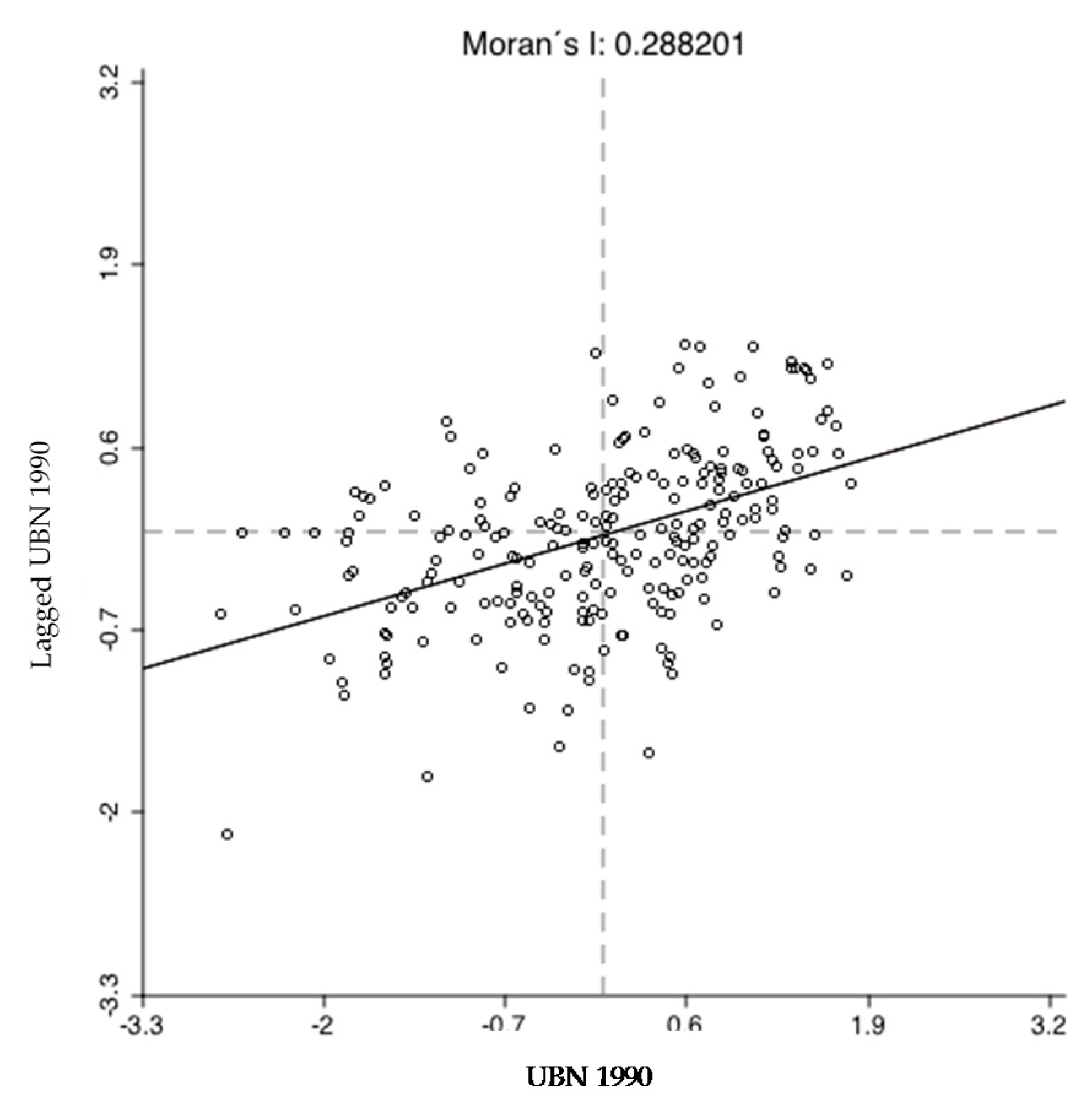
3.2. Spatial Analysis of Poverty
4. Results
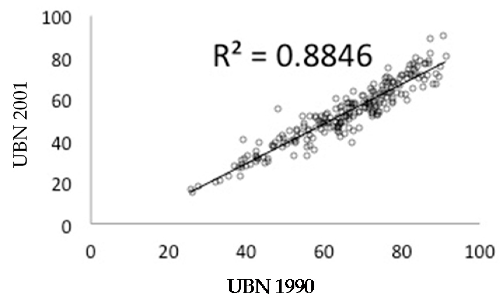
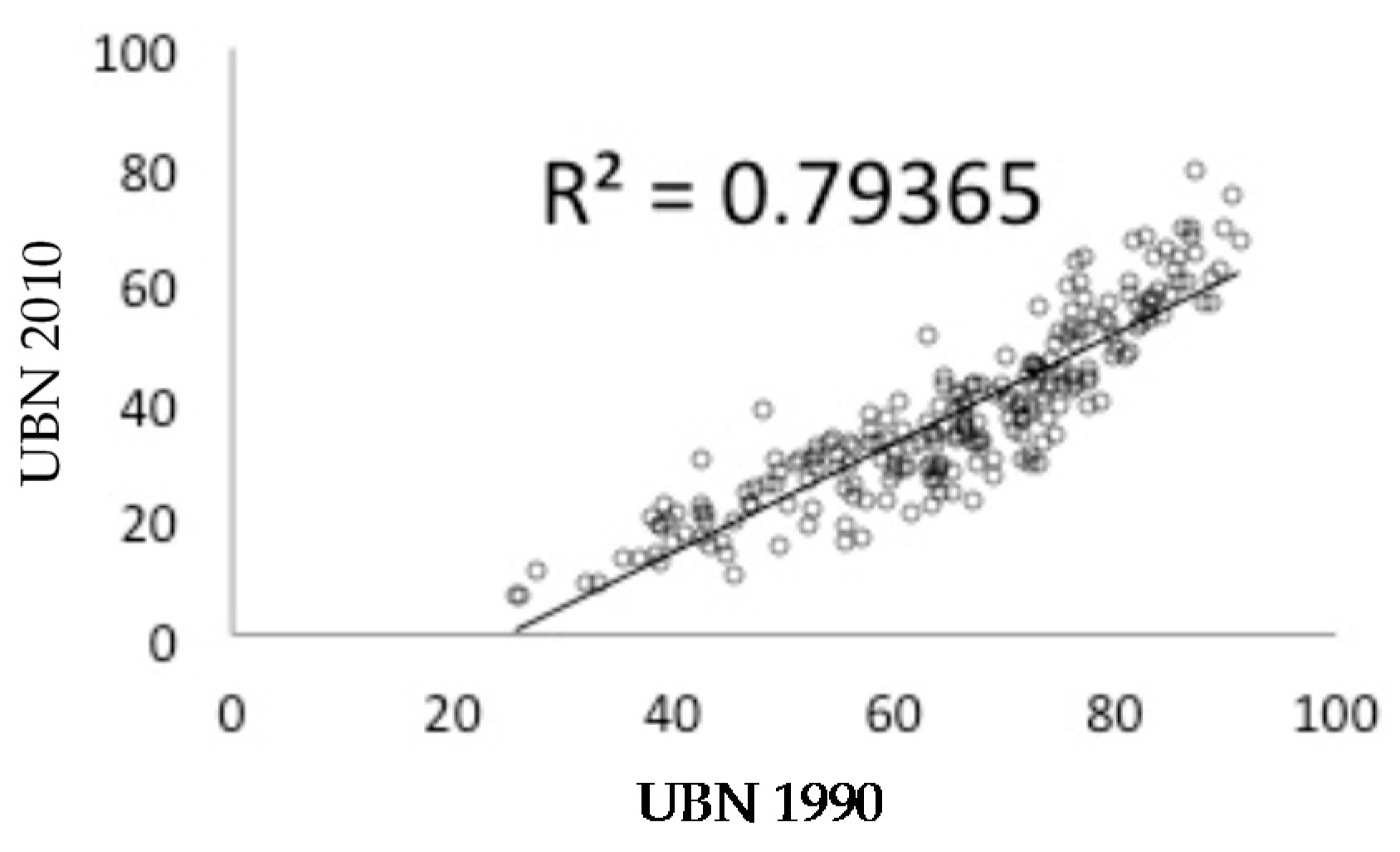
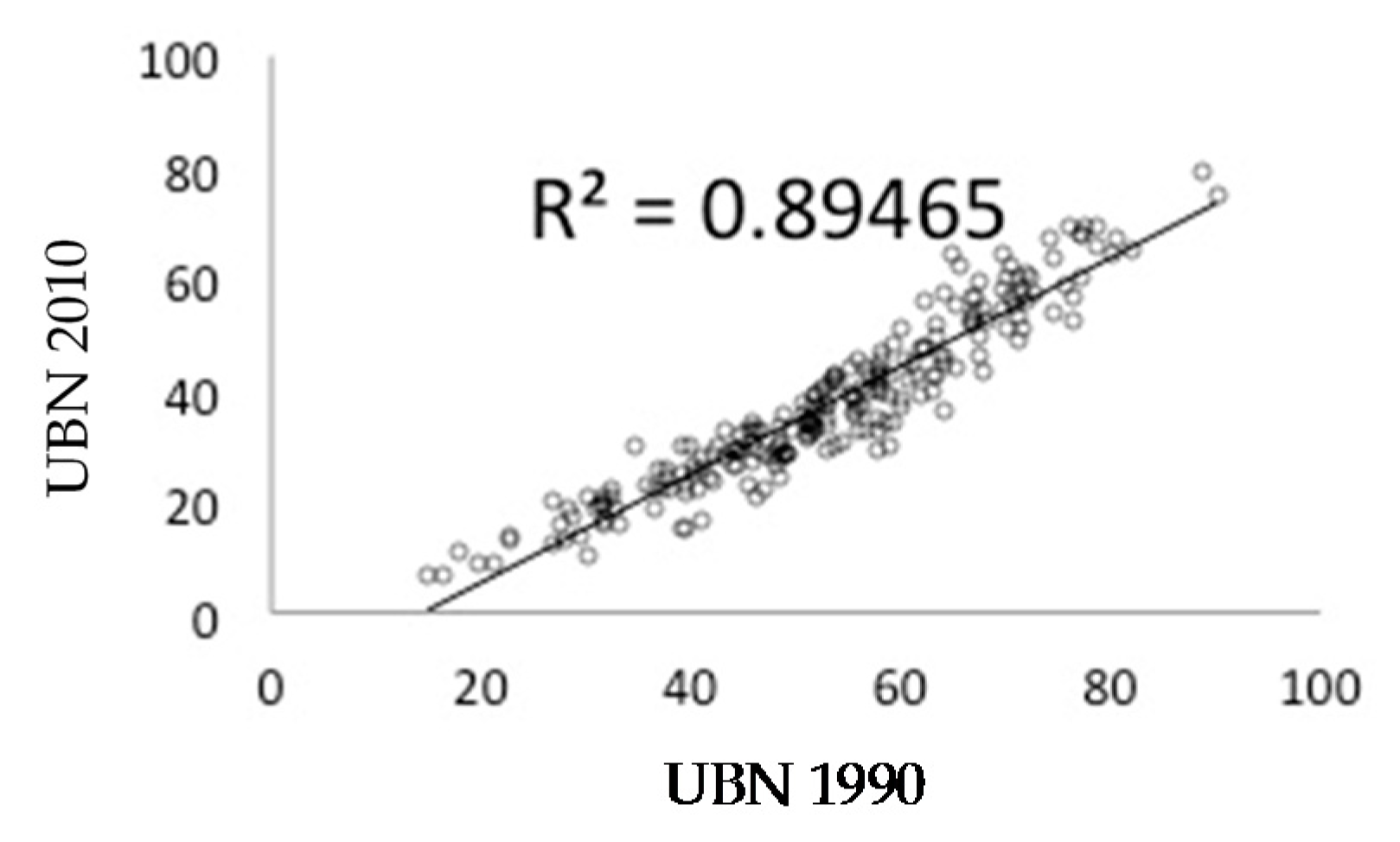
4.1. Persistence of Inequalities over Time
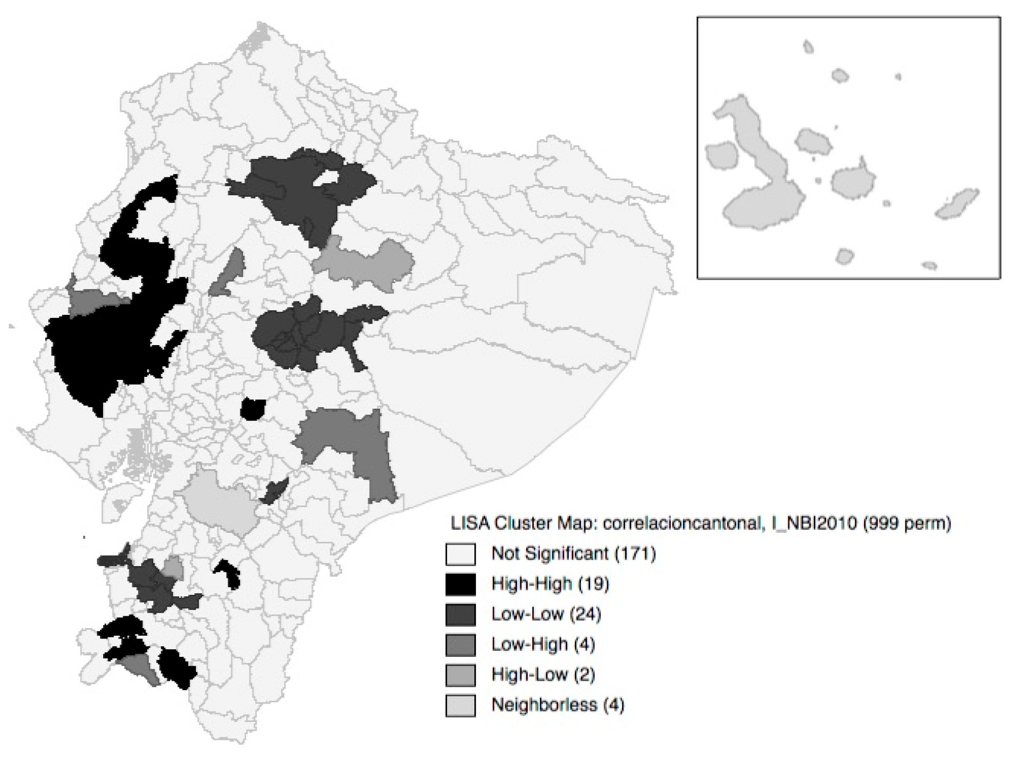
4.2. Poverty Trap
- Forty-two were located mainly on the Ecuadorian Coast in the provinces of Esmeraldas (four), Manabí (17), Los Ríos (seven), Guayas (12), Santa Elena (one), and El Oro (one).
- Twenty-one were located in the Ecuadorian Sierra in the provinces of Chimborazo (two), Cotopaxi (two), Cañar (three), Azuay (three), and Loja (11).
- Seven were located in the Ecuadorian East, corresponding to the provinces of Sucumbíos (two), Orellana (one), Morona Santiago (one), and Zamora Chinchipe (three). The remaining three correspond to the non-delimited zones, which were already mentioned.
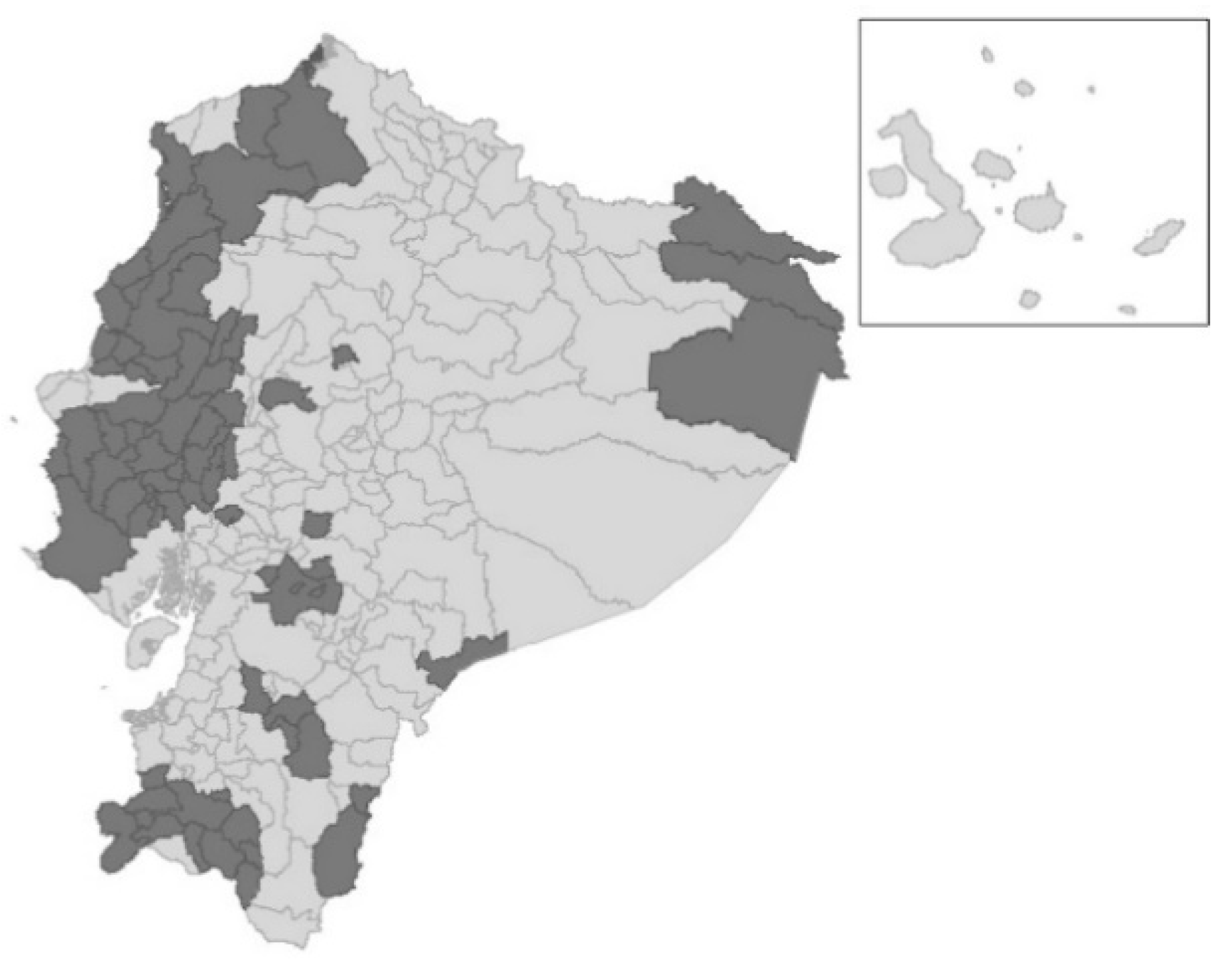
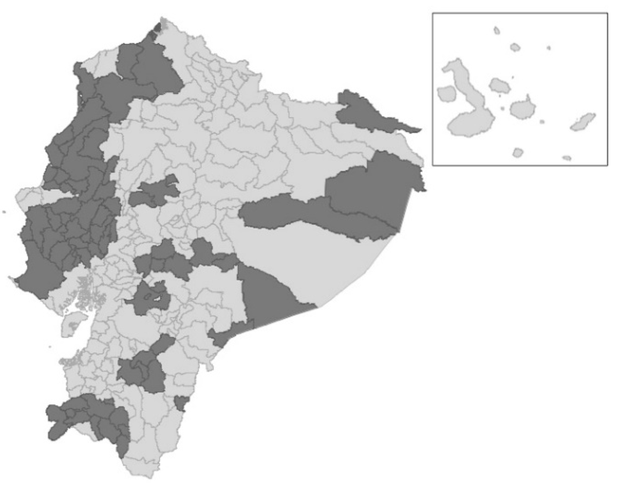
- Thirty-nine were located mainly on the Ecuadorian Coast in the provinces of Esmeraldas (four), Manabí (17), Los Ríos (five), Guayas (11), and Santa Elena (two).
- Twenty-five were located in the Ecuadorian Sierra in the provinces of Chimborazo (four), Cotopaxi (three), Bolívar (one), Cañar (two), Azuay (three), and Loja (12).
- Nine were located in the Ecuadorian East, corresponding to the provinces of Sucumbíos (one), Orellana (one), Pastaza (one), Morona Santiago (four), and Zamora Chinchipe (two); while the remaining two cantons corresponded to the non-delimited zones.
5. Conclusions
Author Contributions
Funding
Conflicts of Interest
References
- Chiriboga, M.; Wallis, B. Diagnóstico de la pobreza rural en Ecuador y respuestas de política pública. In Grupo de Trabajo Sobre Pobreza Rural; Centro Latinoamericano para el Desarrollo Rural: Santiago, Chile, 2010. [Google Scholar]
- García-Vélez, D. La pobreza en Ecuador a través del índice P de Amartya Sen: 2006–2014. Economía 2015, 40, 91–115. [Google Scholar]
- Ruíz, L.; Sánchez, N. La literatura ecuatoriana sobre pobreza urbana. In Pobreza Urbana en el Ecuador-Bibliografía Nacional; CIUDAD-UNICEF: Quito, Ecuador, 1994. [Google Scholar]
- Barreiros, L.; Kouwenaar, A.; Teekebz, R.; Vos, R. La distribución de los Niveles de vida en Ecuador Ecuador; Teoría y Diseño de Políticas para la Satisfacción de las Necesidades Básicas (No. E51 B271); Institute of Social Studies: Santiago, Ecuador, 1987. [Google Scholar]
- Cobos, G. Desarrollo local y pobreza: Desigualdades socioterritoriales. In La Economía Política de la Pobreza; Cimadamore, A., Ed.; CLACSO: Buenos Aires, Argentina, 2008. [Google Scholar]
- Skoufias, E.; Lopez-Acevedo, G. Latin America-Determinants of Regional Welfare Disparities within Latin American Countries: Country Case Studies (No. 3051); Synthesis: Hertfordshire, UK, 2009. [Google Scholar]
- IBRD-World Bank. Ecuador Poverty Assessment; Report No. 27061-EC; The World Bank: Washington, DC, USA, 2004. [Google Scholar]
- Boisier, S. Origen, Evolución y Situación Actual de Las Políticas Territoriales en América Latina en Los Siglos XX y XXI; Planificación, Prospectiva y Gestión Pública, Reflexiones Para la Agenda de Desarrollo; Sn: Santiago, Chile, 2014. [Google Scholar]
- Scott, L.M.; Janikas, M.V. Spatial statistics in ArcGIS. In Handbook of Applied Spatial Analysis—Software Tools, Methods and Applications; Fischer, M.M., Getis, A., Eds.; Springer: Berlin, Heidelberg, 2010; pp. 27–41. [Google Scholar]
- Béland, E.; Escobar, G. Caracterización Socioeconómica de diez Parroquias de la Provincia de Tungurahua, Ecuador; Los Indicadores de Pobreza por Consumo: Santiago, Chile, 2011. [Google Scholar]
- Burgos, S. Evolución de la Pobreza y Desigualdad de Ingresos 2006–2012. Notas Técnicas de Investigación Económica N0. 5, 2013. Available online: http://www.sciencespo.fr/opalc/sites/sciencespo.fr.opalc/files/Evoluci%C3%B3n-de-pobreza-y-desigualdad-de-ingresos-2006-2012_SBD_def.pdf (accessed on 14 September 2018).
- SIISE. Sistema de Indicadores Sociales del Ecuador. Desigualdad y Pobreza, 2018. Available online: http://www.siise.gob.ec/siiseweb/siiseweb.html?sistema=1# (accessed on 14 September 2018).
- Ministerio de Coordinación de Desarrollo Social. Mapa de Desigualdad y Pobreza en Ecuador, Quito-Ecuador: Editorial Aries; Ministerio de Coordinación de Desarrollo Social: Quito, Ecuador, 2012.
- ECLAC. Ecuador: Mapa de Necesidades Básicas Insatisfechas. Naciones Unidas, Cepal (División de Estadística y Proyecciones); PNUD-RLA/86/004; ECLAC: Santiago, Chile, 1989. [Google Scholar]
- CONADE. Mapa de la Pobreza Consolidado; CONADE: Quito, Ecuador, 1993.
- INEC. Compendio de las Necesidad Básicas Insatisfechas de la Población Ecuatoriana; Instituto Nacional de Estadísticas y Censos: Guayaquil, Ecuador, 1995. [Google Scholar]
- Larrea, C.; Andrade, J.; Brborich, W.; Jarrín, D.; Reed, C. Geografía de la pobreza en el Ecuador. In Geografía de la Pobreza en el Ecuador; United Nations Development Programme—Facultad Latinoamericana de Ciencias Sociales: Quito, Ecuador, 1996. [Google Scholar]
- Larrea, C. Desarrollo Social y Gestión Municipal en el Ecuador: Jerarquización y Tipología; ODEPLAN: Quito, Ecuador, 1999. [Google Scholar]
- SIISE—STMCDS. Mapa de Pobreza y Desigualdad en Ecuador; INNFA: Guayaquil, Ecuador; Editorial Aries: Quito, Ecuador, 1996. [Google Scholar]
- SIISE—STMCDS. Mapa de Pobreza y Desigualdad en Ecuador; INNFA: Guayaquil, Ecuador; Editorial Aries: Quito, Ecuador, 2010. [Google Scholar]
- SENPLADES. Atlas de Las Desigualdades Socio Económicas en el Ecuador; TRAMA Ediciones: Quito, Ecuador, 2013. [Google Scholar]
- Banerjee, A.; Duflo, E. Poor Economics: A Radical Rethinking of the Way to Fight Global Poverty; Public Affairs, Perseus Books: New York, NY, USA, 2011. [Google Scholar]
- Barrientos, J.; Gòmez, W.; Rhenals, R. Crecimiento, distribución y pobreza en América Latina: Un ejercicio de panel, 1990–2005. Perf. Coyunt. Econ. 2008, 11, 15–50. [Google Scholar]
- Carter, M.R.; Barrett, C.B. The economics of poverty traps and persistent poverty: An asset-based approach. J. Dev. Stud. 2006, 42, 178–199. [Google Scholar] [CrossRef]
- Islam, T.M.; Minier, J.; Ziliak, J.P. On persistent poverty in a rich country. Southern Econ. J. 2015, 81, 653–678. [Google Scholar] [CrossRef]
- Mayer-Foulkes, D. Globalization and the Human Development Trap (No. 2007/64); Research Paper; UNU-WIDER, United Nations University (UNU): Tokyo, Japan, 2007. [Google Scholar]
- Burdín, G.; Ferrando, M.; Leites, M.; Salas, G. Trampas de Pobreza: Concepto y Medición Nueva Evidencia Sobre la Dinámica del Ingreso en Uruguay; Fondo Concursable Carlos Filgueira: Montevideo, Uruguay, 2009; p. 195. [Google Scholar]
- Arim, R.; Brum, M.; Dean, A.; Leites, M.; Salas, G. Movilidad de ingreso y trampas de pobreza: Nueva evidencia para los países del Cono Sur. Estud. Econ. 2013, 28, 3–38. [Google Scholar]
- Zhang, H. The poverty trap of education: Education–poverty connections in Western China. Int. J. Educ. Dev. 2014, 38, 47–58. [Google Scholar] [CrossRef]
- Dutta, S. Identifying Single or Multiple Poverty Trap: An Application to Indian Household Panel Data. Soc. Indic. Res. 2015, 120, 157–179. [Google Scholar] [CrossRef]
- Giesbert, L.; Schindler, K. Assets, shocks, and poverty traps in rural Mozambique. World Dev. 2012, 40, 1594–1609. [Google Scholar] [CrossRef]
- Galvis, L.A.; Meisel, A. Persistencia de Las Desigualdades Regionales en Colombia: Un Análisis Espacial; Documentos de Trabajo Sobre Economía Regional, 120; Centro de Estudios Económicos Regionales–CER Banco de La República: Bogotá, Colombia, 2010.
- Argüello, C.R.; Zambrano, A. ¿Existe una trampa de pobreza en el sector rural en Colombia? Rev. Desarro. Soc. 2006, 58, 85–113. [Google Scholar] [CrossRef]
- Agostini, C.A.; Brown, P.H.; Góngora, D.P. Spatial distribution of poverty in Chile. Estud. Econ. 2008, 35, 79–110. [Google Scholar]
- Pereira, M.; Soloaga, I. Trampas de pobreza y desigualdad en México 1990–2000–2010; Serie Documentos de Trabajo. Documento, 134; RIMISP-Centro Latinoamericano para el Desarrollo Rural: Santiago, Chile, 2014. [Google Scholar]
- Thomas, A.C.; Gaspart, F. Does Poverty Trap Rural Malagasy Households? World Dev. 2015, 67, 490–505. [Google Scholar] [CrossRef]
- Tavares, J.M.; Junior, S.D.S.P. “Corredores Da Pobreza” E “Ilhas De Prosperidade”: Uma análise espacial e multidimensional dos níveis de desenvolvimento na região sul do Brasil. Anál. Rev. Adm. PUCRS 2010, 21, 51–62. [Google Scholar]
- Yúnez, A.; Arellano, J.; Méndez, J. Cambios en el bienestar de 1990 a 2005: Un estudio espacial para México. Estud. Econ. 2010, 25, 363–406. [Google Scholar]
- Risso Brandon, F.; Pasquier-Doumer, L. Aspiration Failure: A Poverty Trap for Indigenous Children in Peru? (No. 123456789/12016); Dauphine University: Paris, France, 2013. [Google Scholar]
- Rowntree, B.S. Poverty: A Study of Town Life; Macmillan and Company Ltd.: London, UK; New York, NY, USA, 1901. [Google Scholar]
- Townsend, P. The meaning of poverty. Br. J. Sociol. 1962, 13, 210–227. [Google Scholar] [CrossRef]
- Runciman, W.G. Relative Deprivation & Social Justice: Study Attitudes Social Inequality in 20th Century England; Routledge and Kegan Paul: London, UK, 1966. [Google Scholar]
- Atkinson, A.B. On the measurement of inequality. J. Econ. Theory 1970, 2, 244–263. [Google Scholar] [CrossRef]
- Sen, A. An Ordinal Approach to Measurement. Econometrica 1976, 44, 219–231. [Google Scholar] [CrossRef]
- Chaudhuri, S.; Ravallion, M. How well do static indicators identify the chronically poor? J. Public Econ. 1994, 53, 367–394. [Google Scholar] [CrossRef]
- Kaztman, R. Virtudes y Limitaciones de los Mapas Censales de Carencias Críticas; Revista de la Cepal, 58 (LC/G.1916-P); CEPAL: Santiago, Chile, 1996. [Google Scholar]
- Feres, J.C.; Mancero, X. El Método de las Necesidades Básicas Insatisfechas (NBI) y sus Aplicaciones en América Latina; Naciones Unidas Comisión Económica para América Latina y el Caribe (CEPAL): Santiago, Chile, 2001. [Google Scholar]
- Sen, A. Inequality Reexamined; Oxford University Press: Oxford, UK, 1992. [Google Scholar]
- Bourguignon, F.; Chakravarty, S.R. The measurement of multidimensional poverty. J. Econ. Inequal. 2003, 1, 25–49. [Google Scholar] [CrossRef]
- Alkire, S.; Foster, J. Recuento y Medición Multidimensional de la Pobreza; OPHI Working Paper Series; OPHI: Oxford, UK, 2007; Volume 7, pp. 1–45. [Google Scholar]
- Domínguez Domínguez, J.; Martín Caraballo, A.M. Medición de la pobreza: Una revisión de los principales indicadores. Rev. Métod. Cuantitativos Econ. Empres. 2006, 2, 27–66. [Google Scholar]
- Grupo de Río. Compendio de Mejores Prácticas en la Medición de la Pobreza; Grupo de Río: Santiago, Chile, 2007; Available online: http://www.eclac.cl/deype/publicaciones/sinsigla/xml/9/34409/rio_group_compendium_es.pdf (accessed on 1 September 2018).
- Núñez Velázquez, J.J. Estado actual y nuevas aproximaciones a la medición de la pobreza. Estud. Econ. Apl. 2009, 27, 325–344. [Google Scholar]
- Feres, J.C.; Mancero, X. Enfoques Para la Medición de la Pobreza: Breve Revisión de la Literatura; Serie Estudios Estadísticos y Prospectivos CEPAL, (4); Naciones Unidas Comisión Económica para América Latina y el Caribe (CEPAL): Santiago, Chile, 2001. [Google Scholar]
- Silva Arias, A. Una primera revisión de las medidas de pobreza. Rev. Fac. Cienc. Econ. Investig. Reflex. 2005, 13, 53–71. [Google Scholar]
- Martínez Bernal, B.L. Planteamientos sobre la pobreza: Una aproximación conceptual. Apunt. CENES 2015, 34, 15–40. [Google Scholar] [CrossRef]
- Tukey, J.W. Exploratory Data Analysis; Addison-Wesley: Boston, MA, USA, 1977. [Google Scholar]
- Yrigoyen, C.C. Análisis estadístico de datos geográficos en geomarketing: El programa GeoDa. Distrib. Consum. 2006, 2, 34–45. [Google Scholar]
- Anselin, L. Spatial Data Analysis with SpaceStatTM and ArcView, Workbook, 3rd ed.; Department of Agricultural and Consumer Economics; University of Illinois: Chicago, IL, USA; Urbana, IL, USA, 1999. [Google Scholar]
- Moran, P.A. Notes on continuous stochastic phenomena. Biometrika 1950, 37, 17–23. [Google Scholar] [CrossRef] [PubMed]
- Celemín, J.P. Autocorrelación espacial e indicadores locales de asociación espacial: Importancia, estructura y aplicación. Rev. Univ. Geogr. 2009, 18, 11–31. [Google Scholar]
- Bohórquez, I.A.; Ceballos, E.V. Algunos conceptos de la econometría espacial y el análisis exploratorio de datos espaciales. Ecos Econ. 2008, 12, 2–25. [Google Scholar]
- Pearson, K. Mathematical contributions to the theory of evolution. III. Regression, heredity, and panmixia. Philosophical Transactions of the Royal Society of London. Ser. A Contain. Pap. Math. Phys. Charact. 1986, 187, 253–318. [Google Scholar]
- Goodchild, M. Spatial autocorrelation. In Encyclopedia of Geographic Information Science; Karen, K., Ed.; SAGE: Thousand Oaks, CA, USA, 2008; pp. 397–398. [Google Scholar]
- Dale, M.R.; Fortin, M.J. Spatial Analysis: A Guide for Ecologists; Cambridge University Press: Cambridge, UK, 2014. [Google Scholar]
- Rivero, M.S. Análisis espacial de datos y turismo: Nuevas técnicas para el análisis turístico. Una aplicación al caso extremeño. Rev. Estud. Empres. 2008, 2, 48–66. [Google Scholar]
- Geary, R.C. The contiguity ratio and statistical mapping. Incorp. Stat. 1954, 5, 115–146. [Google Scholar] [CrossRef]
- Getis, A.; Ord, J.K. The analysis of spatial association by use of distance statistics. Geogr. Anal. 1992, 24, 189–206. [Google Scholar] [CrossRef]
- Anselin, L. Spatial econometrics in RSUE: Retrospect and prospect. Reg. Sci. Urban Econ. 2007, 37, 450–456. [Google Scholar] [CrossRef]
- Díaz, A.M.; Torres, F.J.S. Geografía de Los Cultivos Ilícitos y Conflicto Armado en Colombia; Universidad de los Andes, Facultad de Economía, CEDE: Bogota, Colombia, 2004. [Google Scholar]
- Buzai, G. Los Sistemas de Información Geográfica y sus métodos de análisis en el continuo resolución-integración. In Memorias X Conferencia Iberoamericana de Sistemas de Información Geográfica (X CONFIBSIG); Universidad de Puerto Rico: Río Piedras, Puerto Rico, 2005. [Google Scholar]
- Anselin, L. Local indicators of spatial association—LISA. Geogr. Anal. 1995, 27, 93–115. [Google Scholar] [CrossRef]
- Ord, J.K.; Getis, A. Local spatial autocorrelation statistics: Distributional issues and an application. Geogr. Anal. 1995, 27, 286–306. [Google Scholar] [CrossRef]
- Unwin, A. Exploratory spatial analysis and local statistics. Comput. Stat. 1996, 11, 387–400. [Google Scholar]
- Sánchez-Peña, L.L. Alcances y límites de los métodos de análisis espacial para el estudio de la pobreza urbana. Pap. Poblac. 2012, 18, 147–180. [Google Scholar]
- Yue, W.; Zhang, Y.; Ye, X.; Cheng, Y.; Leipnik, M. Dynamics of multi-scale intra-provincial regional inequality in Zhejiang, China. Sustainability 2014, 6, 5763–5784. [Google Scholar] [CrossRef]
- Zhang, J.; Deng, W. Multiscale Spatio-Temporal Dynamics of Economic Development in an Interprovincial Boundary Region: Junction Area of Tibetan Plateau, Hengduan Mountain, Yungui Plateau and Sichuan Basin, Southwestern China Case. Sustainability 2016, 8, 215. [Google Scholar] [CrossRef]
- Pérez, G.J. Dimensión Espacial de la Pobreza en Colombia; Ensayos sobre Política Económica, No. 54; Banco de la Republica de Colombia: Cartagena, Colombia, 2005; pp. 234–293.
- Muñetón, G.; Vanegas, J.G. Análisis espacial de la pobreza en Antioquia, Colombia. Equidad Desarro. 2014, 21, 29–47. [Google Scholar] [CrossRef]
- Tian, Y.; Wang, Z.; Zhao, J.; Jiang, X.; Guo, R. A Geographical Analysis of the Poverty Causes in China’s Contiguous Destitute Areas. Sustainability 2018, 10, 1895. [Google Scholar] [CrossRef]
- Jurado, A.; Pérez, J. Análisis de las diferencias espaciales de las tasas de pobreza. In XV Encuentro de Economía Pública: Políticas Públicas y Migración; S.n.: Salamanca, España, 2008; p. 21. [Google Scholar]
- Bolívar Espinoza, G.A.; Caloca Osorio, Ó.R. Distribución espacial de la pobreza Distrito Federal de México 1990-2040. Polis-Rev. Latinoam. 2011, 10, 19–53. [Google Scholar] [CrossRef]
- Wu, J.X.; He, L.Y. Urban–rural gap and poverty traps in China: A prefecture level analysis. Appl. Econ. 2018, 50, 3300–3314. [Google Scholar] [CrossRef]
- Serrano, A. Análisis de condiciones de vida, el mercado laboral y los medios de producción e inversión pública. In Cuaderno de Trabajo Secretaria Nacional de Planificación y Desarrollo; SENPLADES: Quito, Ecuador, 2013; pp. 1–248. [Google Scholar]
- Haining, R.P. Spatial Data Analysis: Theory and Practice; Cambridge University Press: Cambridge, UK, 2003. [Google Scholar]
- Anselin, L. What is special about spatial data? Alternative perspectives on spatial data analysis. In Spatial Statistics, Past, Present and Future; Griffith, D.A., Ed.; Institute of Mathematical Geography (IMAGE): Ann Arbor, MI, USA, 1989; pp. 66–77. [Google Scholar]
- Anselin, L. Spatial Data Analysis with GIS: An Introduction to Application in the Social Sciences; National Center for Geographic Information and Analysis, University of California: Santa Barbara, CA, USA, 1992; pp. 10–92. [Google Scholar]
- Tobler, W.R. Cellular geography. In Philosophy in geography; Springer: Dordrecht, The Netherlands, 1979; pp. 379–386. [Google Scholar]
- Cliff, A.D.; Ord, J.K. Spatial Autocorrelation; Pion: London, UK, 1973; Volume 5. [Google Scholar]
- Upton, G.; Fingleton, B. Spatial Data Analysis by Example; Volume 1: Point Pattern and Quantitative Data; John Wiley & Sons Ltd.: Chichester, UK, 1985. [Google Scholar]


| Dimensions | Deprivation Indicators |
|---|---|
| Economic capacity | If the years of schooling of the head of the family are less than or equal to two years. |
| If there are more than three people for each person employed in the home. | |
| Access to basic education | If there are children at home aged between six and 12 who do not attend school. |
| Access to housing | If the floor material of the house is with earth or other materials. |
| If the wall material of the house is made of reed, matting, or other materials. | |
| Access to basic services | If the house does not have a toilet or if it has one, it is a concrete pit or latrine. |
| If the water obtained by the house is not from a public network or another piping source. | |
| Overcrowding | If the number of people per bedroom is greater than three. |
| WX | II (Low values surrounded by high values) | I (High values surrounded by high values) |
| III (Low values surrounded by low values) | IV (High values surrounded by low values) | |
| X | ||
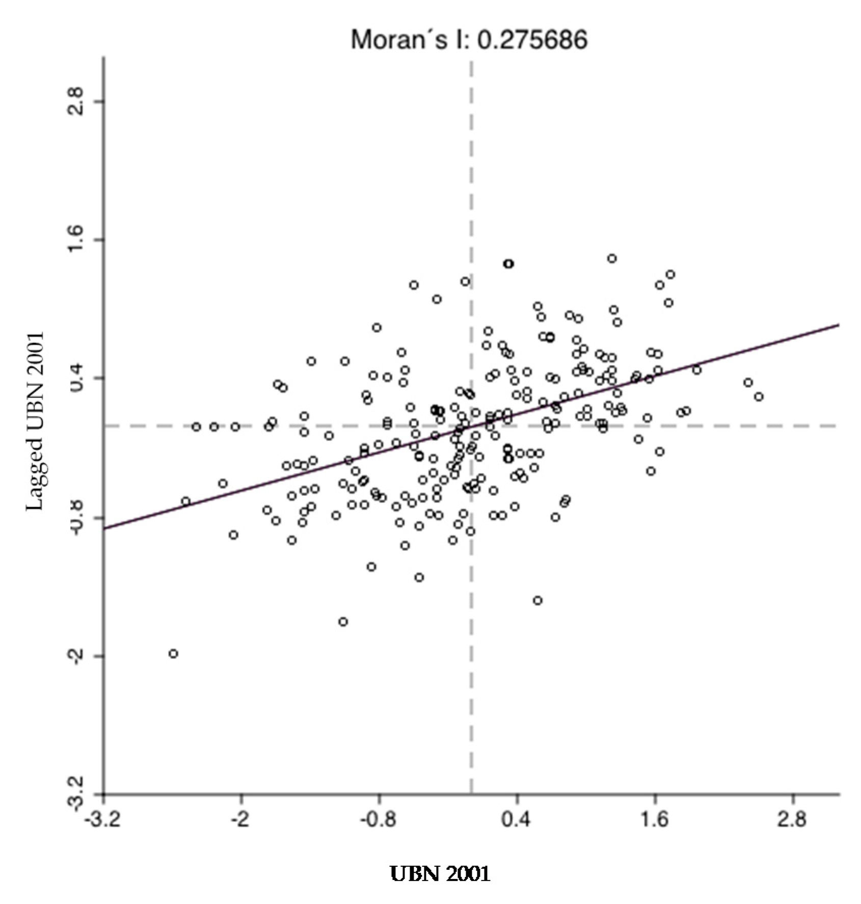
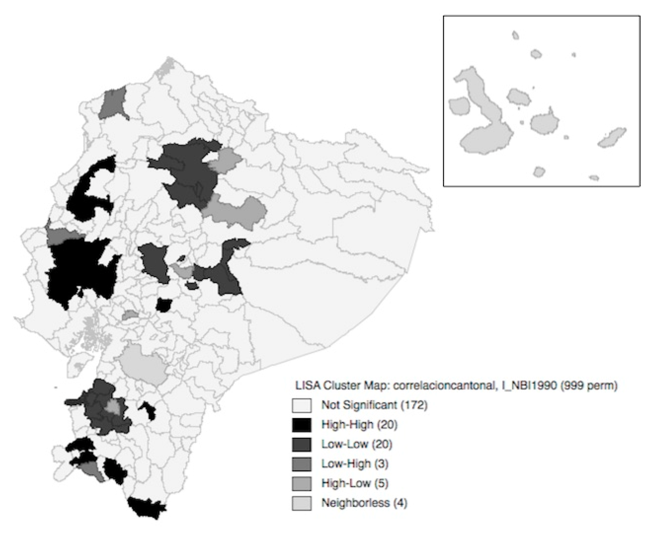
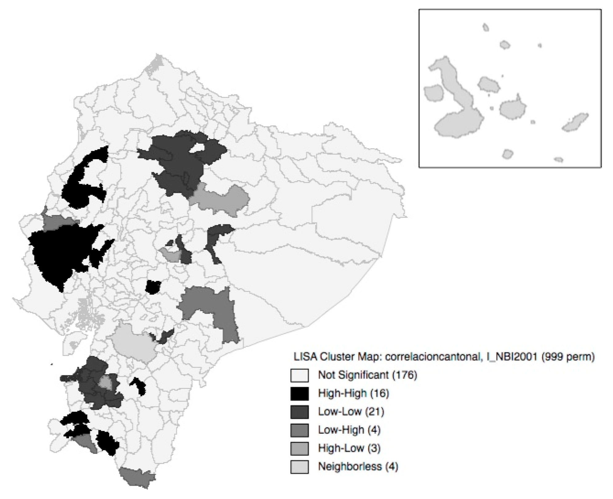
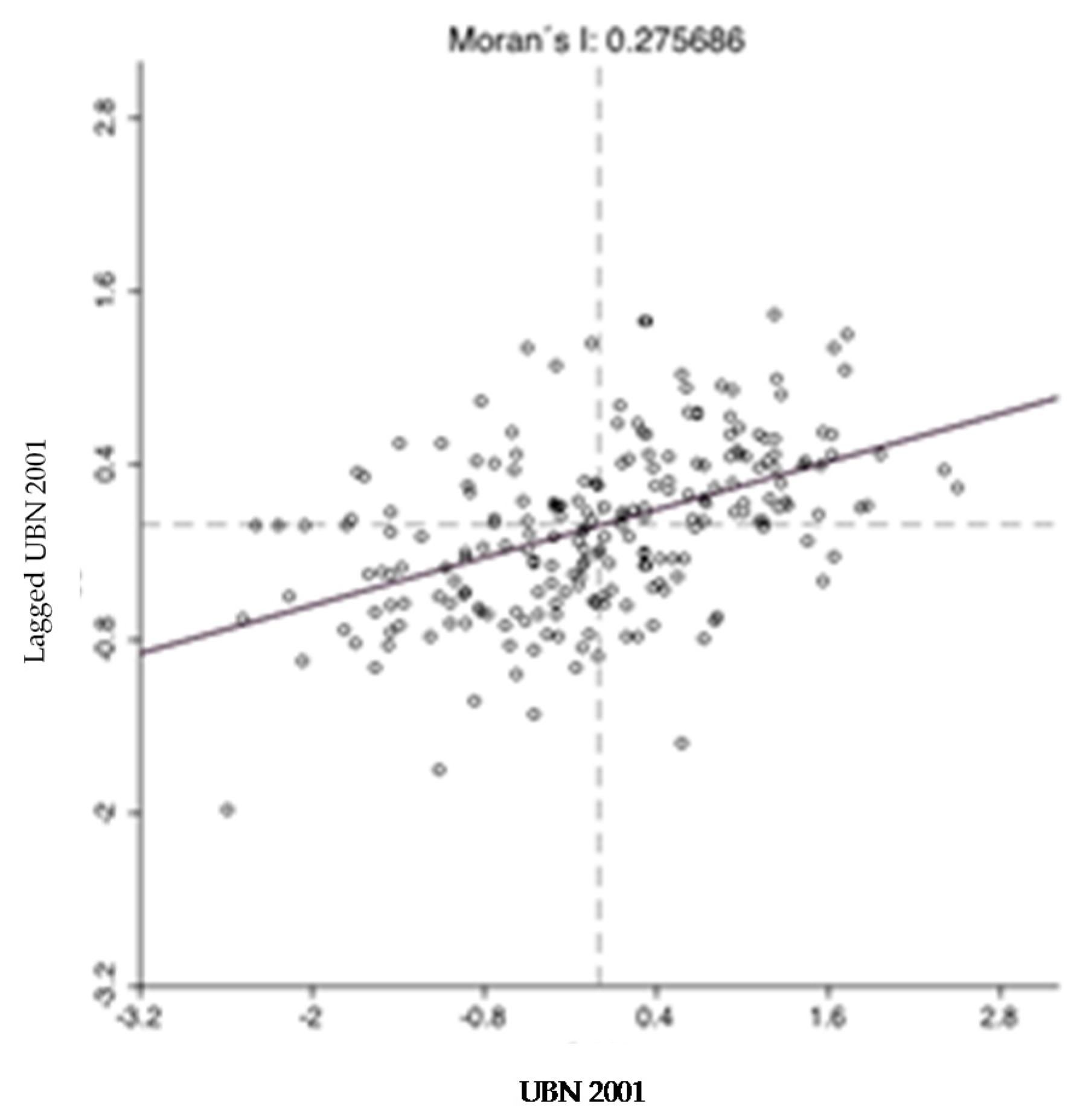
| Spatial lag of the UBN (1990) | LH32(14.3%) | HH73(32.6%) | Spatial lag of the UBN (2001) | LH38(17%) | HH75(33.5%) |
| LL79(35.3%) | HL40(17.9%) | LL84(37.5%) | HL27(12%) | ||
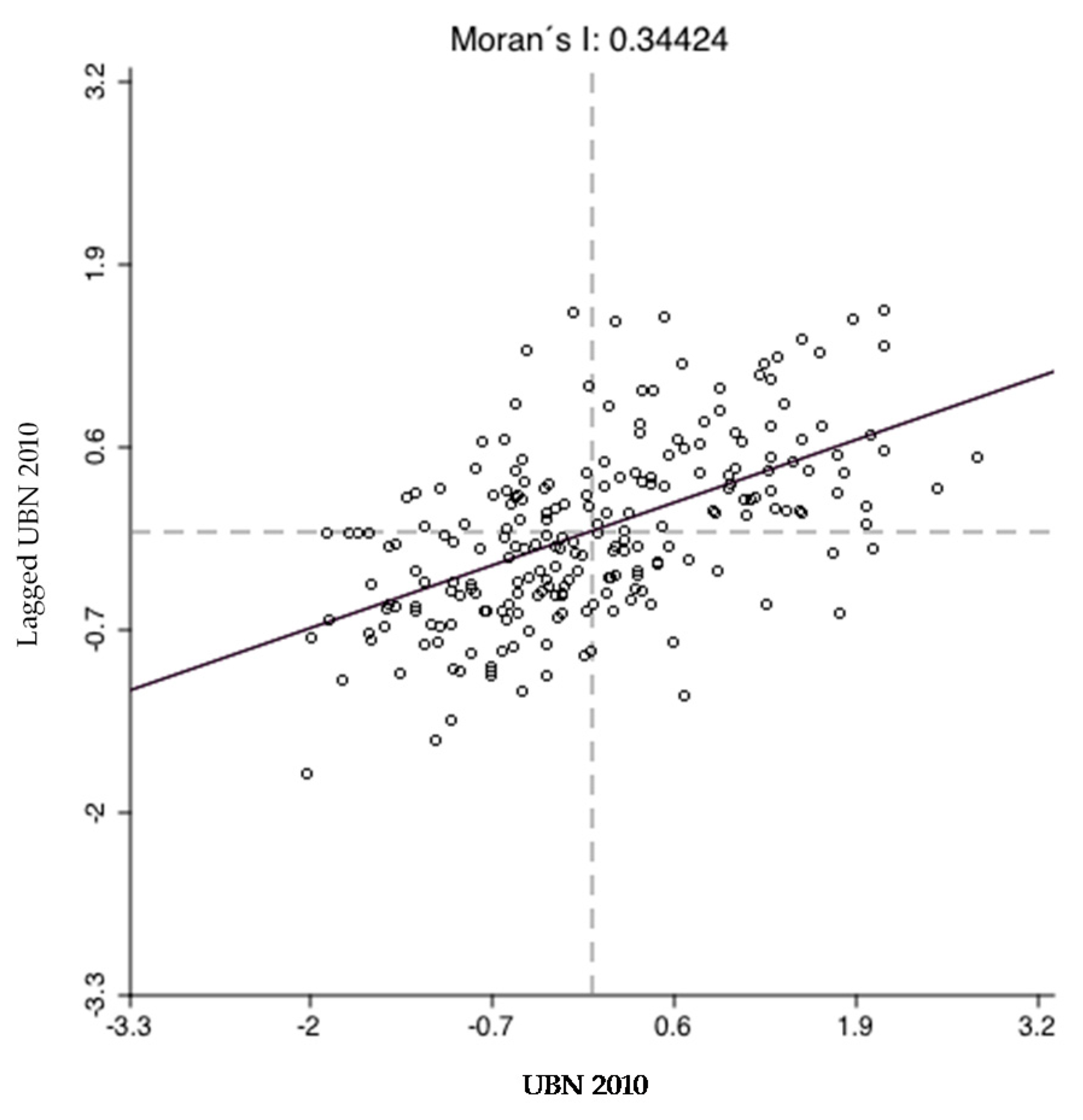
| UBN (2001) | UBN (2010) | ||||
© 2018 by the authors. Licensee MDPI, Basel, Switzerland. This article is an open access article distributed under the terms and conditions of the Creative Commons Attribution (CC BY) license (http://creativecommons.org/licenses/by/4.0/).
Share and Cite
Correa-Quezada, R.; García-Vélez, D.F.; Del Río-Rama, M.d.l.C.; Álvarez-García, J. Poverty Traps in the Municipalities of Ecuador: Empirical Evidence. Sustainability 2018, 10, 4316. https://doi.org/10.3390/su10114316
Correa-Quezada R, García-Vélez DF, Del Río-Rama MdlC, Álvarez-García J. Poverty Traps in the Municipalities of Ecuador: Empirical Evidence. Sustainability. 2018; 10(11):4316. https://doi.org/10.3390/su10114316
Chicago/Turabian StyleCorrea-Quezada, Ronny, Diego Fernando García-Vélez, María de la Cruz Del Río-Rama, and José Álvarez-García. 2018. "Poverty Traps in the Municipalities of Ecuador: Empirical Evidence" Sustainability 10, no. 11: 4316. https://doi.org/10.3390/su10114316
APA StyleCorrea-Quezada, R., García-Vélez, D. F., Del Río-Rama, M. d. l. C., & Álvarez-García, J. (2018). Poverty Traps in the Municipalities of Ecuador: Empirical Evidence. Sustainability, 10(11), 4316. https://doi.org/10.3390/su10114316