The Influence of Marine Traffic on Particulate Matter (PM) Levels in the Region of Danish Straits, North and Baltic Seas


Abstract
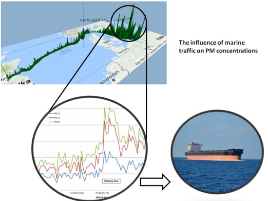
1. Introduction
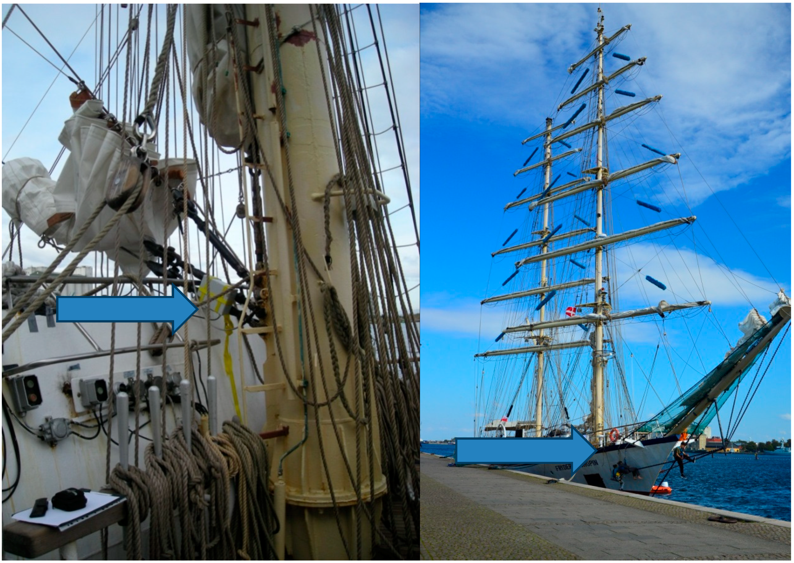
2. Materials and Methods
- hour and day (Universal Time Coordinated (UTC), based on the data from the built-in Global Positioning System (GPS)),
- geographical location (based on the data from the built-in GPS),
- measured concentrations of PM10, PM2.5, and PM1,
- temperature and relative humidity.
3. Results and Discussion
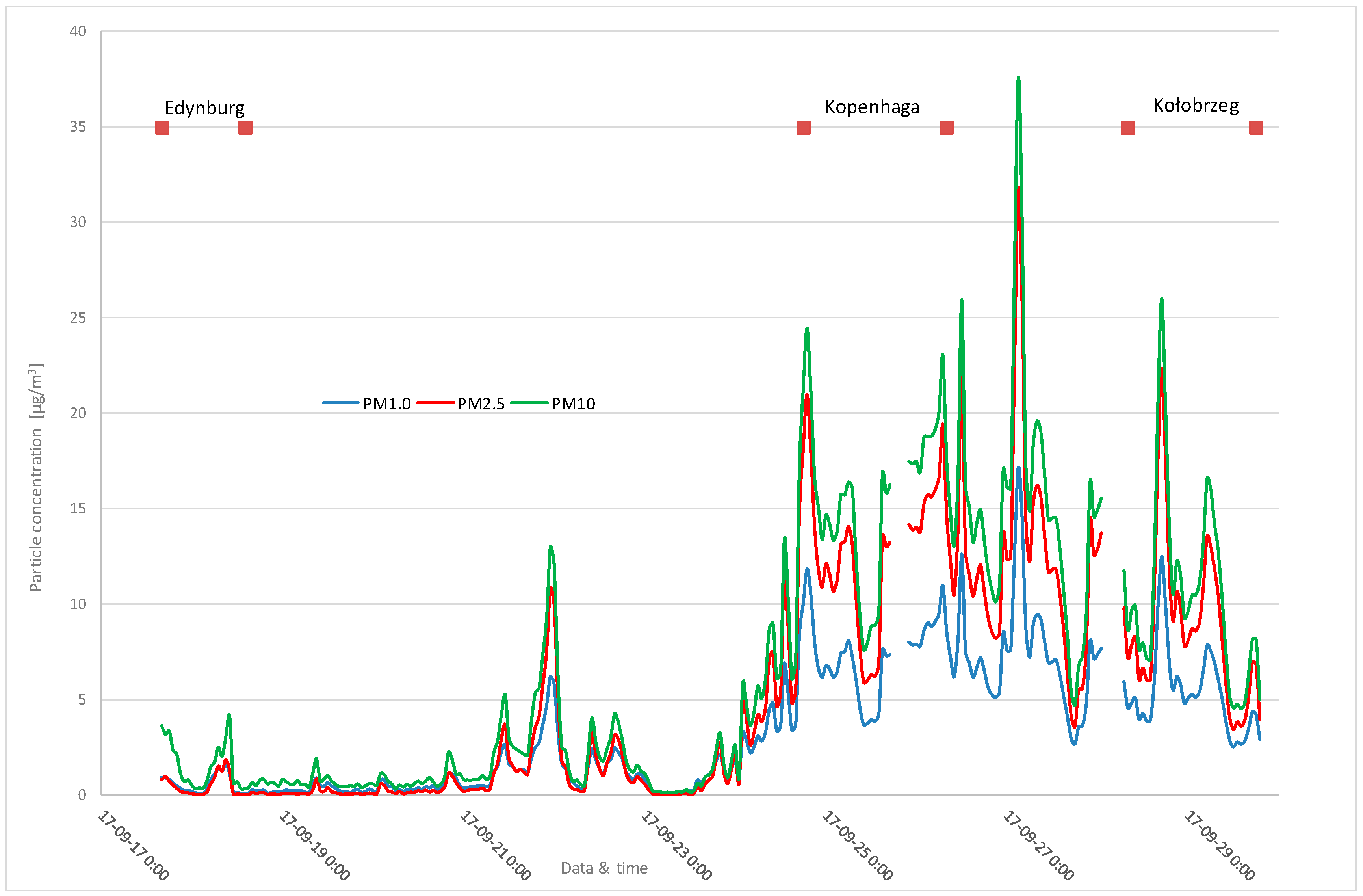
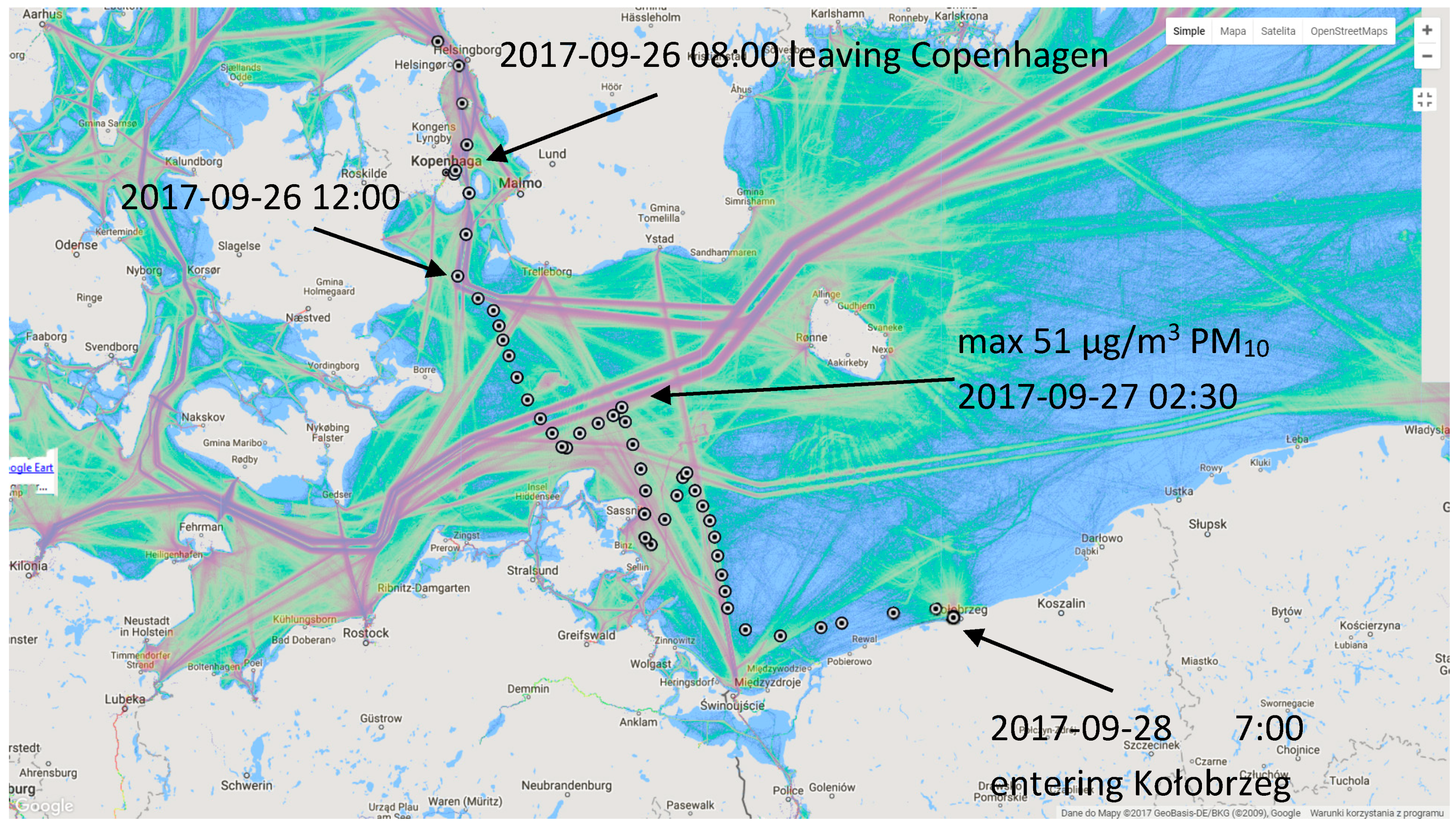
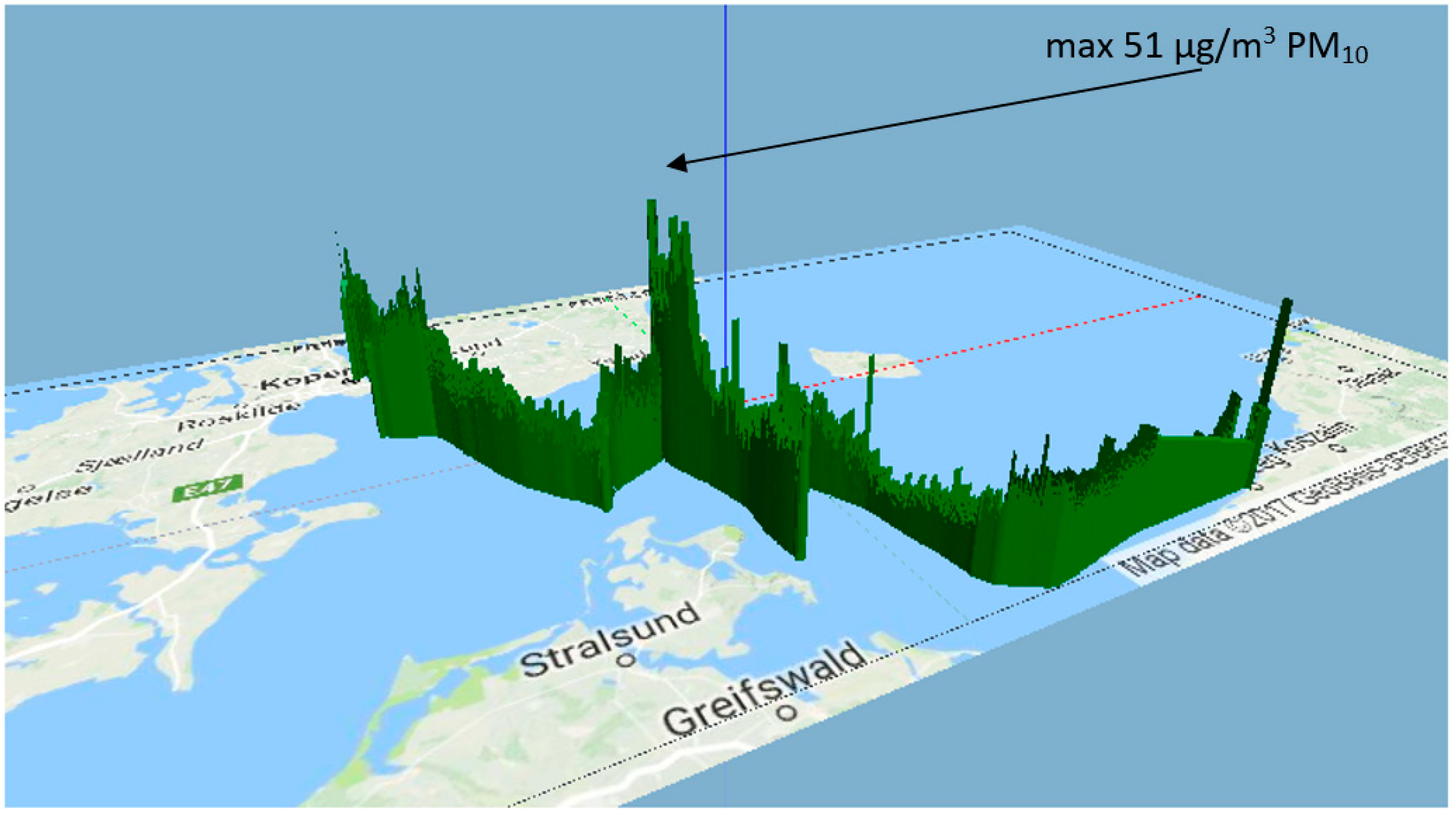
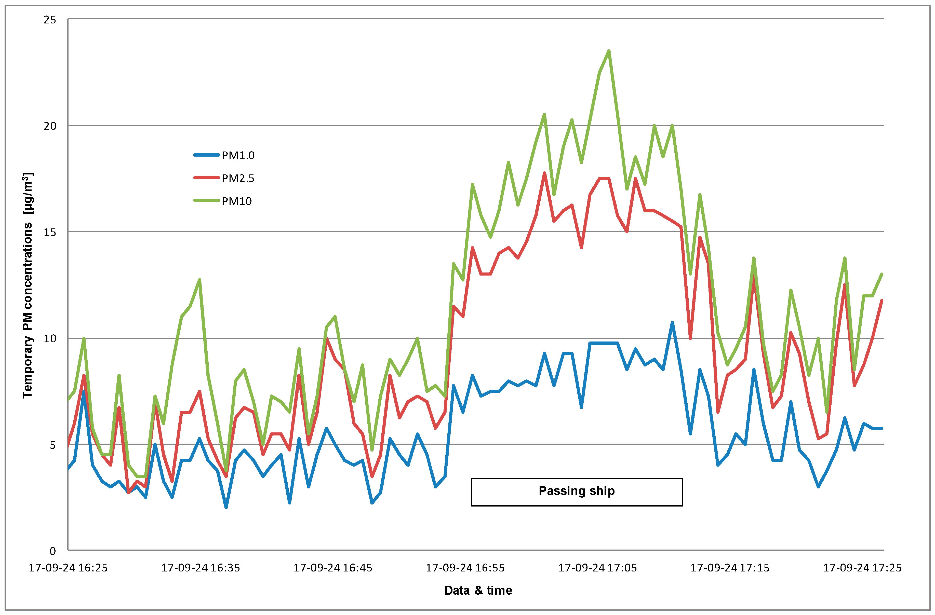
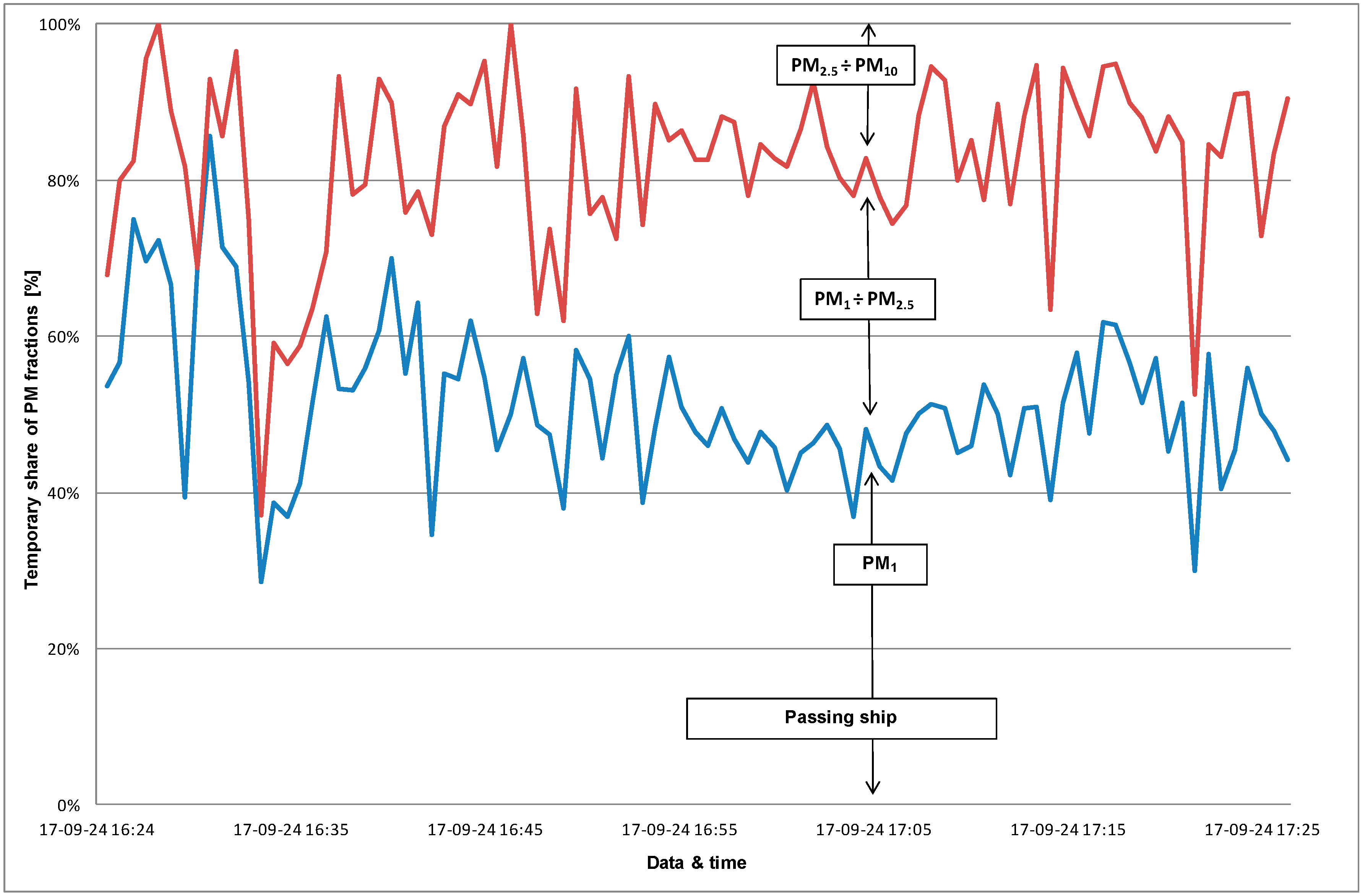
3.1. PM Concentrations in the Region of Danish Straits and North and Baltic Seas
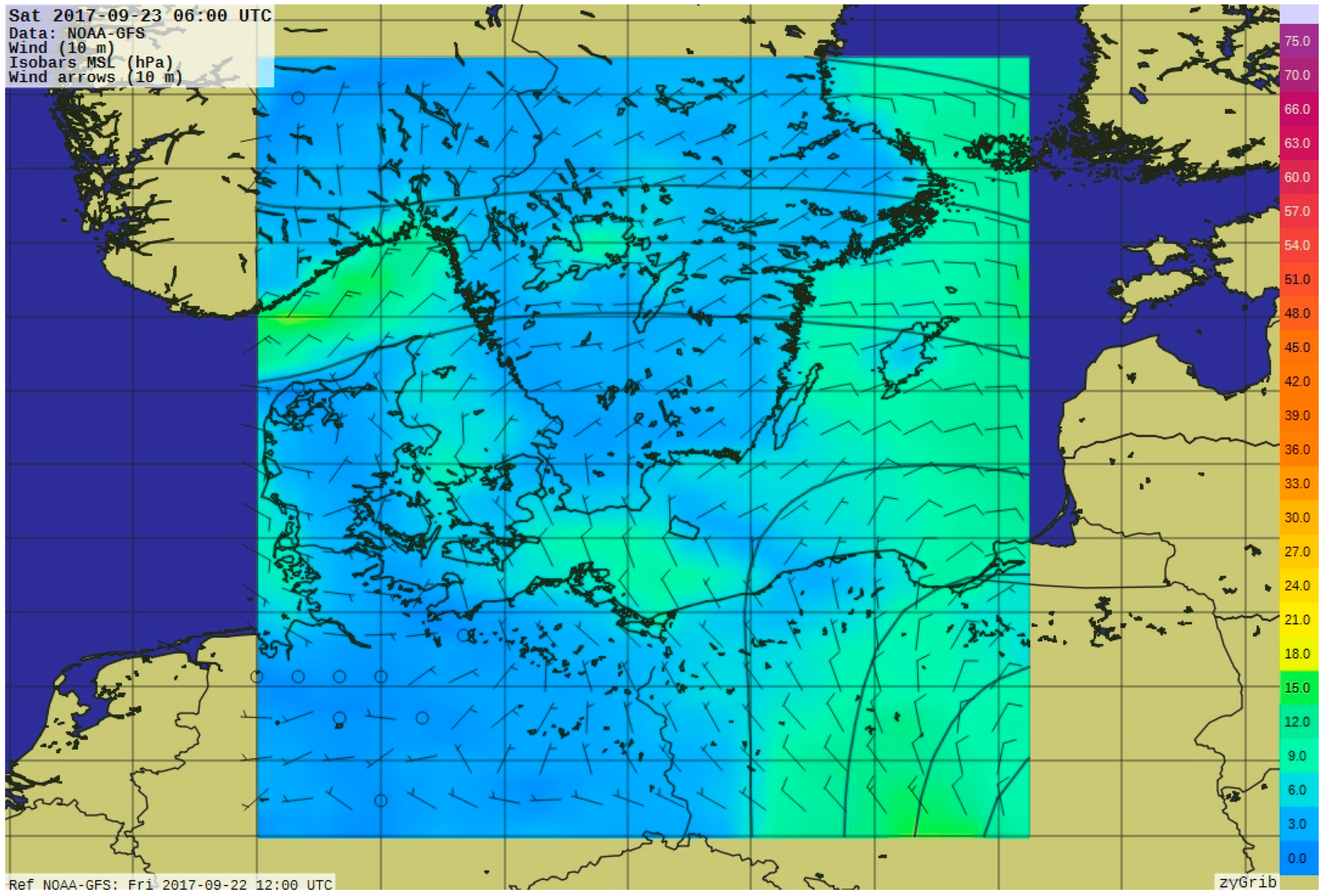
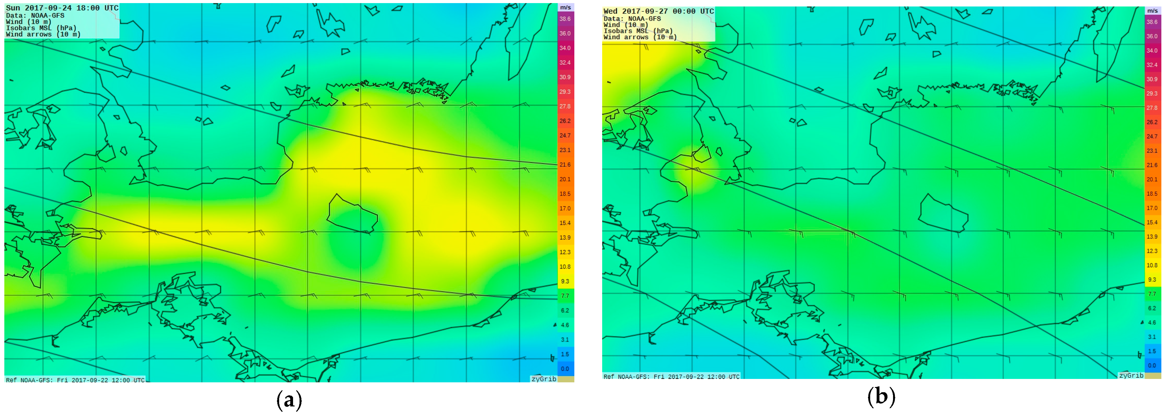
- Presence of a stronger wind, 11–14 m/s—during the other part of the cruise, the wind was around 3.5–8.0 m/s,
- The direction of wind blowing, which at the time changed from south to northeast—the wind came from Sweden (Figure 7).
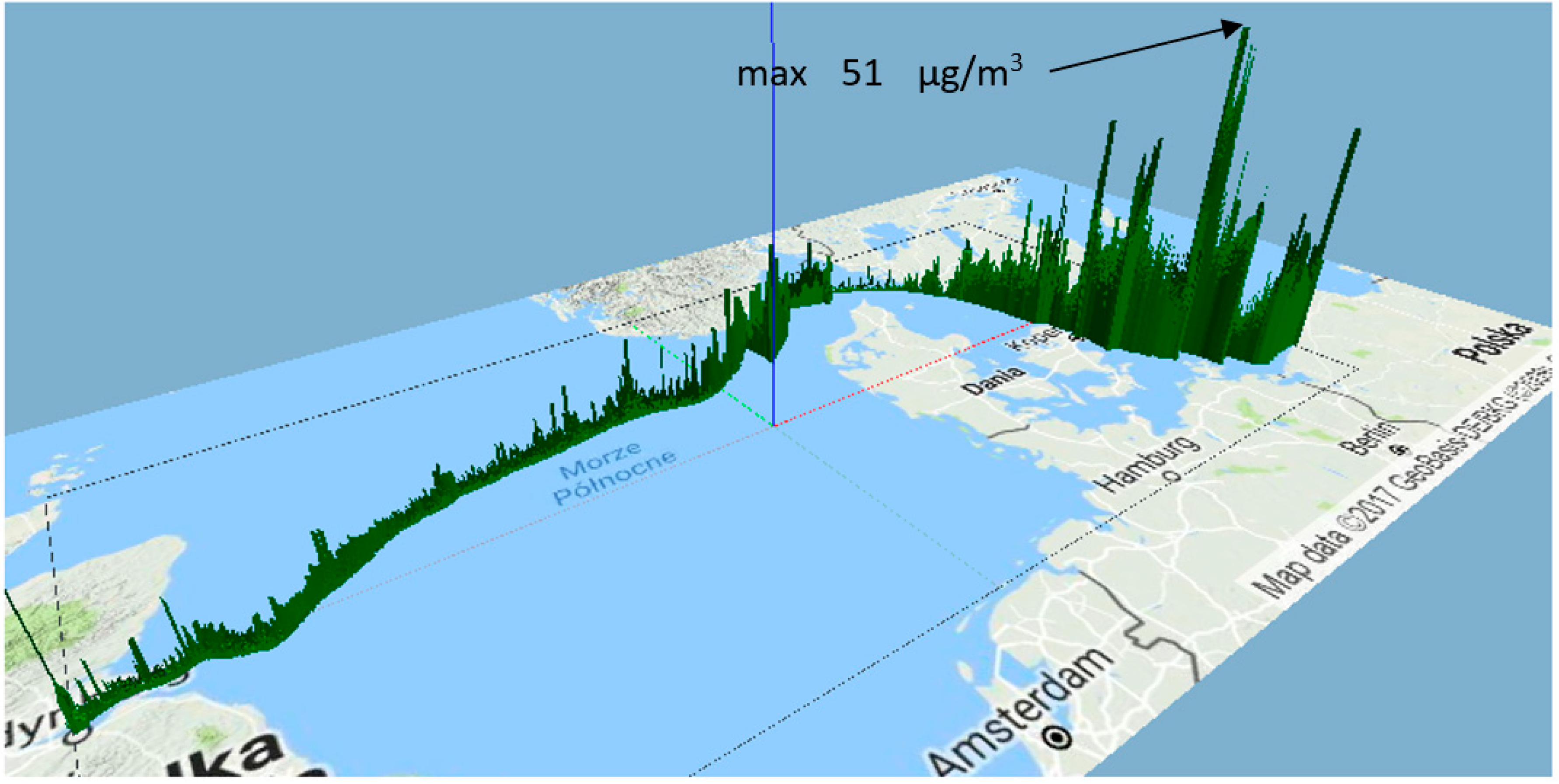
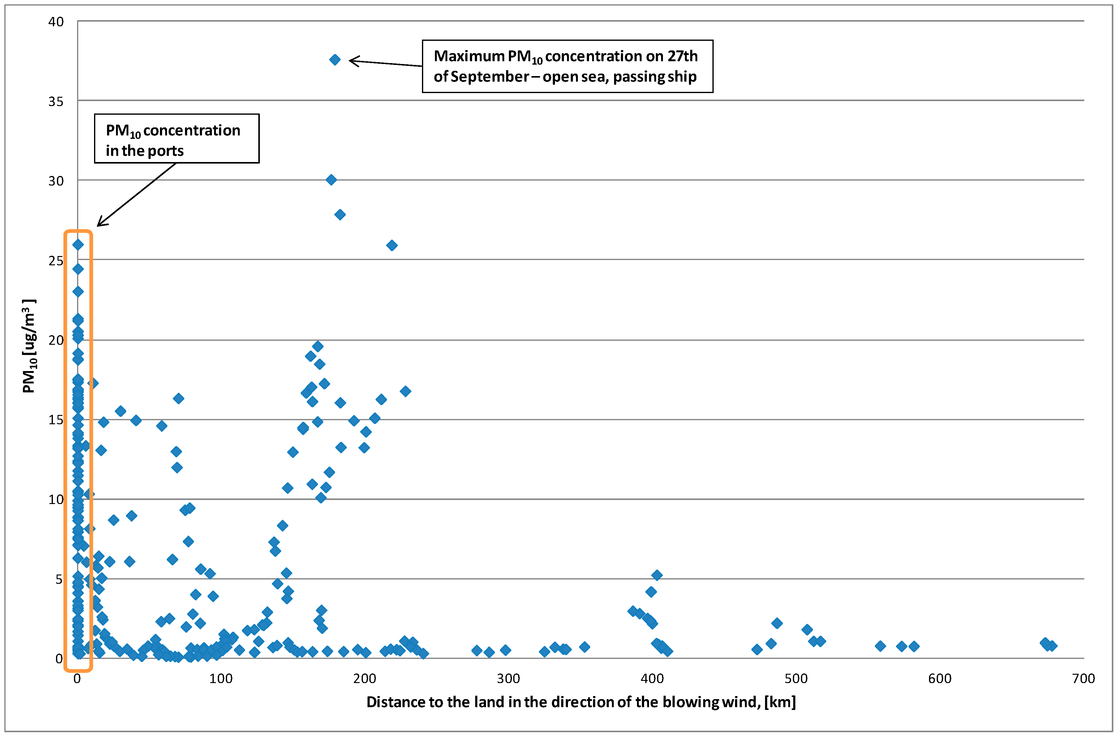
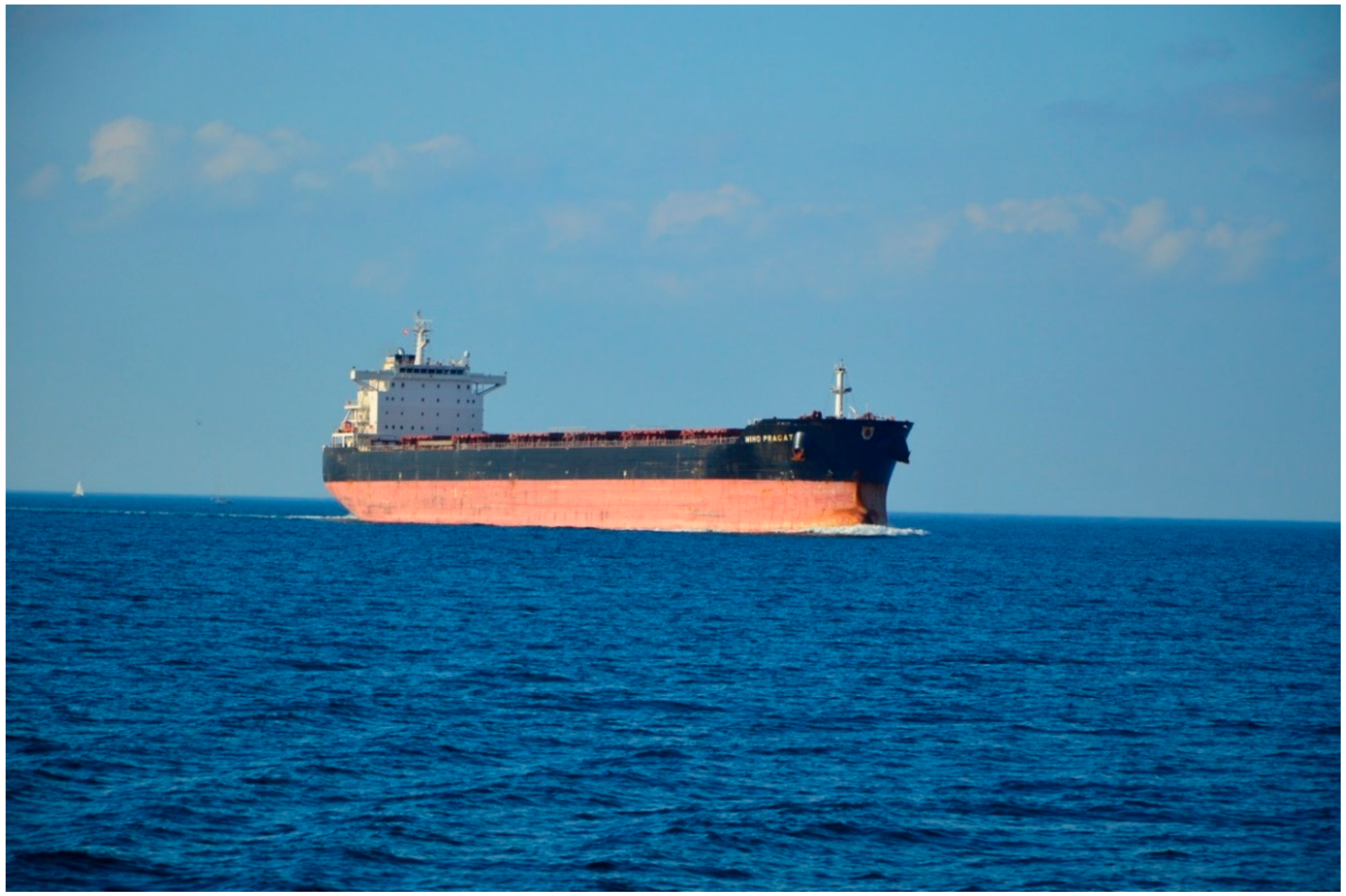
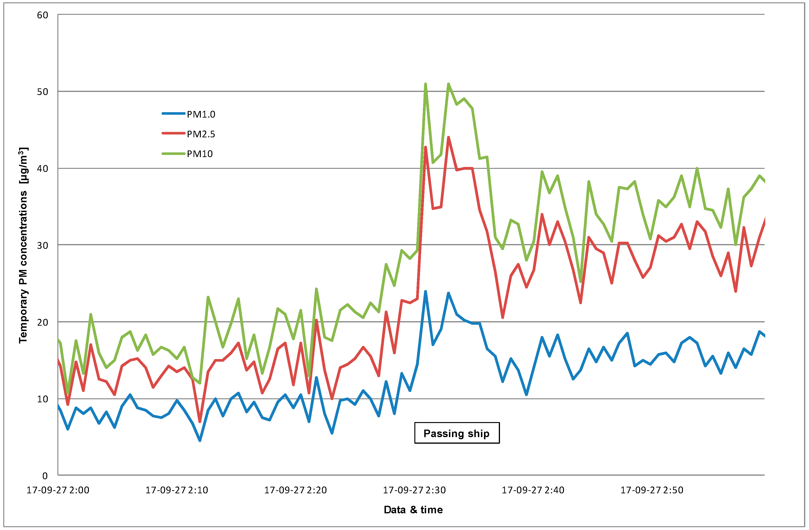
3.2. Pollution Migration and Sources
4. Conclusions
- the implementation of international instruments regulating/addressing pollutants emissions from ships;
- the benefits and cost-effectiveness of various emission-reduction strategies.
Author Contributions
Funding
Acknowledgments
Conflicts of Interest
References
- European Commission (EC). Air Quality Standards. Available online: http://ec.europa.eu/environment/air/quality/standards.htm (accessed on 7 March 2018).
- European Environment Agency (EEA). Air Quality in Europe—2014 Report; Report No. 5/2014; EEA: Copenhagen, Denmark, 2014. [Google Scholar]
- Majewski, G.; Badyda, A.; Czechowski, P.O.; Dabrowiecki, P.; Gayer, A.; Mucha, D.; Adamkiewicz, L. The Prevalence of Selected Respiratory Diseases and the Exposure to PM10 in the Ambient Air. AST J. 2016, 193, A5417. [Google Scholar]
- Majewski, G.; Badyda, A.; Gayer, A.; Czechowski, P.O.; Dabrowiecki, P. Pulmonary Function and Incidence of Selected Respiratory Diseases Depending on the Exposure to Ambient PM10. Int. J. Mol. Sci. 2016, 17, 1954. [Google Scholar] [CrossRef]
- World Health Organization (WHO). Health Risks of Air Pollution in Europe—HRAPIE Project: Recommendations for Concentration—Response Functions for Cost-benefit Analysis of Particulate Matter, Ozone and Nitrogen Dioxide; Report of WHO Regional Office for Europe; WHO Regional Office for Europe: Copenhagen, Denmark, 2013. [Google Scholar]
- Heimann, I.; Bright, V.B.; McLeod, M.W.; Mead, M.I.; Popoola, O.A.M.; Stewart, G.B.; Jones, R.L. Source attribution of air pollution by spatial scale separation using high spatial density networks of low cost air quality sensors. Atmos. Environ. 2015, 113, 10–19. [Google Scholar] [CrossRef]
- Van den Bossche, J.; Peter, J.; Verwaeren, J.; Botteldooren, D.; Theunis, J.; De Baets, B. Mobile monitoring for mapping spatial variation in urban air quality: Development and validation of a methodology based on an extensive dataset. Atmos. Environ. 2015, 105, 148–161. [Google Scholar] [CrossRef]
- Wong, M.S.; Wang, T.; Ho, H.C.; Kwok, C.Y.T.; Lu, K.; Abbas, S. Towards a Smart City: Development and Application of an Improved Integrated Environmental Monitoring System. Sustainability 2018, 10, 623. [Google Scholar] [CrossRef]
- Han, L.; Zhou, W.; Li, W. Growing Urbanization and the Impact on Fine Particulate Matter (PM2.5) Dynamics. Sustainability 2018, 10, 1696. [Google Scholar] [CrossRef]
- Ma, Y.; Richards, M.; Ghanem, M.; Guo, Y.; Hassard, J. Air Pollution Monitoring and Mining Based on Sensor Grid in London. Sensors 2008, 8, 3601–3623. [Google Scholar] [CrossRef] [PubMed]
- Kumar, P.; Morawska, L.; Martani, C.; Biskos, G.; Neophytou, M.; Di Sabatino, S.; Bell, M.; Norford, L.; Britter, R. The rise of microsensing for managing air pollution in cities. Environ. Int. 2015, 75, 199–205. [Google Scholar] [CrossRef] [PubMed]
- Snyder, E.; Watkins, T.; Solomon, P.; Thoma, E.; Williams, R.; Hagler, G.; Shelow, D.; Hindin, D.; Kilaru, V.; Preuss, P. The changing paradigm of air pollution monitoring. Environ. Sci. Technol. 2013, 47, 11369–11377. [Google Scholar] [CrossRef] [PubMed]
- Bove, M.C.; Brotto, P.; Calzolai, G.; Cassola, F.; Cavalli, F.; Fermo, P.; Hjorth, J.; Massabò, D.; Nava, S.; Piazzalunga, A.; et al. PM10 source apportionment applying PMF and chemical tracer analysis to ship-borne measurements in the Western Mediterranean. Atmos. Environ. 2016, 125, 140–151. [Google Scholar] [CrossRef]
- Schembari, C.; Bove, M.C.; Cuccia, E.; Cavalli, F.; Hjorth, J.; Massab, D.; Nava, S.; Udisti, R.; Prati, P. Source apportionment of PM10 in the Western Mediterranean based on observations from a cruise ship. Atmos. Environ. 2014, 98, 510–518. [Google Scholar] [CrossRef]
- Romagnoli, P.; Balducci, C.; Perilli, M.; Perreca, E.; Cecinato, A. Particulate PAHs and n-alkanes in the air over Southern and Eastern Mediterranean Sea. Chemosphere 2016, 159, 516–525. [Google Scholar] [CrossRef] [PubMed]
- Deniz, C.; Kilic, A.; Cıvkaroglu, G. Estimation of shipping emissions in Candarli Gulf, Turkey. Environ. Monit. Assess. 2010, 171, 219–228. [Google Scholar] [CrossRef] [PubMed]
- Yau, P.S.; Lee, S.C.; Corbett, J.J.; Wang, C.; Cheng, Y.; Ho, K.F. Estimation of exhaust emission from ocean-going vessels in Hong Kong. Sci. Total Environ. 2012, 431, 299–306. [Google Scholar] [CrossRef] [PubMed]
- Chen, D.; Wang, X.; Li, Y.; Lang, J.; Zhoua, Y.; Guo, X.; Zhao, Y. High-spatiotemporal-resolution ship emission inventory of China based on AIS data in 2014. Sci. Total Environ. 2017, 609, 776–787. [Google Scholar] [CrossRef] [PubMed]
- Zhang, Z.; Yang, X.; Brown, R.; Yang, L.; Morawska, L.; Ristovski, Z.; Fu, Q.; Huang, C. Shipping emissions and their impacts on air quality in China. Sci. Total Environ. 2017, 581, 186–198. [Google Scholar] [CrossRef] [PubMed]
- Liu, H.; Jin, X.; Wu, L.; Wang, X.; Fu, M.; Lv, Z.; Morawska, L.; Huang, F.; Hea, K. The impact of marine shipping and its DECA control on air quality in the Pearl River Delta, China. Sci. Total Environ. 2018, 625, 1476–1485. [Google Scholar] [CrossRef] [PubMed]
- Rogulski, M. The use of low-cost measuring devices for testing air quality in hard-to-reach locations. Energy Proc. 2017, 128, 437–444. [Google Scholar] [CrossRef]
- Rogulski, M. Using low-cost PM monitors to detect local changes of air quality. Pol. J. Environ. Stud. 2018, 27. accepted. [Google Scholar] [CrossRef]
- Isaac, M. Regulatory considerations of lower cost air pollution sensor data performance. Environ. Manag. 2014, 7, 32–37. [Google Scholar] [CrossRef]
- Gao, M.; Cao, J.; Seto, E. A distributed network of low-cost continuous reading sensors to measure spatiotemporal variations of PM2.5 in Xi’an, China. Environ. Pollut. 2015, 199, 56–65. [Google Scholar] [CrossRef] [PubMed]
- Crilley, L.R.; Shaw, M.; Pound, R.; Kramer, L.J.; Price, R.; Young, S.; Lewis, A.C.; Pope, F.D. Evaluation of a low-cost optical particle counter (Alphasense OPC-N2) for ambient air monitoring. Atmos. Meas. Tech. 2018, 11, 709–720. [Google Scholar] [CrossRef]
- Scotland Air Quality Data and Statistics Database, Particulate Matter (PM10) Concentrations (µg/m3); Scottish Government: Edinburgh, UK, 2016.
- Eyring, V.; Isaksen, I.S.A.; Berntsen, T.; Collins, W.J.; Corbett, J.J.; Endresen, O.; Grainger, R.G.; Moldanova, J.; Schlager, H.; Stevenson, D.S. Transport impacts on atmosphere and climate: Shipping. Atmos. Environ. 2010, 44, 4735–4771. [Google Scholar] [CrossRef]
- Di Natale, F.; Carotenuto, C. Particulate matter in marine diesel engines exhausts: Emissions and control strategies. Transp. Res. Part D Transp. Environ. 2015, 40, 166–191. [Google Scholar] [CrossRef]
- Sarvi, A.; Lyyränen, J.; Jokiniemi, J.; Zevenhoven, R. Particulate emissions from large-scale medium-speed diesel engines: 1. Particle size distribution. Fuel Process. Technol. 2011, 92, 1855–1861. [Google Scholar] [CrossRef]
- Fridell, E.; Steen, E.; Peterson, K. Primary particles in ship emissions. Atmos. Environ. 2008, 42, 1160–1168. [Google Scholar] [CrossRef]
- Moldanova, J.; Fridell, E.; Popovicheva, O.; Demirdjian, B.; Tishkova, V.; Faccinetto, A.; Focsa, C. Characterisation of particulate matter and gaseous emissions from a large ship diesel engine. Atmos. Environ. 2009, 43, 2632–2641. [Google Scholar] [CrossRef]
- Firląg, S. How to meet the minimum energy performance requirements of Technical Conditions in year 2021? Procedia Eng. 2015, 111, 202–208. [Google Scholar] [CrossRef]
- Deniz, C.; Durmuşoğlu, Y. Estimating shipping emissions in the region of the Sea of Marmara, Turkey. Sci. Total Environ. 2008, 390, 255–261. [Google Scholar] [CrossRef] [PubMed]
- Brandt, J.; Silver, J.D.; Heile Christensen, J.; Skou Andersen, M.; Geels, C.; Gross, A.; Buus Hansen, A.; Mantzius Hansen, K.; Brandt Hedegaard, G.; Ambelas Skjøth, C. Assessment of Health-Cost Externalities of Air Pollution at the National Level Using the EVA Model System; Centre for Energy, Environment and Health Report Series; University of Copenhagen: Copenhagen, Denmark, 2011; ISSN 1904-7495. [Google Scholar]
- Corbett, J.J.; Winebrake, J.J.; Green, E.H.; Kasibhatla, P.; Eyring, V.; Lauer, A. Mortality from Ship Emissions: A Global Assessment. Environ. Sci. Technol. 2007, 41, 8512–8518. [Google Scholar] [CrossRef] [PubMed]
- Nuttall, P.; Newell, A.; Prasad, B.; Veitayaki, J.; Holland, E. A review of sustainable sea-transport for Oceania: Providing context for renewable energy shipping for the Pacific. Mar. Policy 2014, 283–287. [Google Scholar] [CrossRef]
- Viana, M.; Hammingh, P.; Colette, A.; Querol, X.; Degraeuwe, B.; de Vlieger, I. Impact of maritime transport emissions on coastal air quality in Europe. Atmos. Environ. 2014, 9, 96–105. [Google Scholar] [CrossRef]


| Pollutant | |||||
|---|---|---|---|---|---|
| CO | NO2 | O3 | PM2.5 | PM10 | |
| EPA | 9 ppm (8 h) 35 ppm (1 h) | 100 ppb (1 h) 53 ppb (1 year) | 75 ppb (8 h) | 35 µg/m3 (24 h) 12 µg/m3 (1 year) | 150 µg/m3 (24 h) |
| WHO | 100 mg/m3 (15 min) 15 mg/m3 (1 h) 10 mg/m3 (8 h) 7 mg/m3 (24 h) | 200 µg/m3 (1 h) 40 µg/m3 (1 year) | 100 µg/m3 (8 h) | 25 µg/m3 (24 h) 10 µg/m3 (1 year) | 50 µg/m3 (24 h) 20 µg/m3 (1 year) |
| EEA | 10 mg/m3 (8 h) | 200 µg/m3 (1 h) 40 µg/m3 (1 year) | 120 µg/m3 (8 h) | 25 µg/m3 (1 year) | 50 µg/m3 (24 h) 40 µg/m3 (1 year) |
© 2018 by the authors. Licensee MDPI, Basel, Switzerland. This article is an open access article distributed under the terms and conditions of the Creative Commons Attribution (CC BY) license (http://creativecommons.org/licenses/by/4.0/).
Share and Cite
Firląg, S.; Rogulski, M.; Badyda, A. The Influence of Marine Traffic on Particulate Matter (PM) Levels in the Region of Danish Straits, North and Baltic Seas. Sustainability 2018, 10, 4231. https://doi.org/10.3390/su10114231
Firląg S, Rogulski M, Badyda A. The Influence of Marine Traffic on Particulate Matter (PM) Levels in the Region of Danish Straits, North and Baltic Seas. Sustainability. 2018; 10(11):4231. https://doi.org/10.3390/su10114231
Chicago/Turabian StyleFirląg, Szymon, Mariusz Rogulski, and Artur Badyda. 2018. "The Influence of Marine Traffic on Particulate Matter (PM) Levels in the Region of Danish Straits, North and Baltic Seas" Sustainability 10, no. 11: 4231. https://doi.org/10.3390/su10114231
APA StyleFirląg, S., Rogulski, M., & Badyda, A. (2018). The Influence of Marine Traffic on Particulate Matter (PM) Levels in the Region of Danish Straits, North and Baltic Seas. Sustainability, 10(11), 4231. https://doi.org/10.3390/su10114231