Stochastic Empty Container Repositioning Problem with CO2 Emission Considerations for an Intermodal Transportation System

Abstract
1. Introduction
2. Mathematical Model for Stochastic ECRP with CO2 Emissions
2.1. Notations and Assumptions
2.2. A Chance-Constrained Nonlinear Integer Programming Model
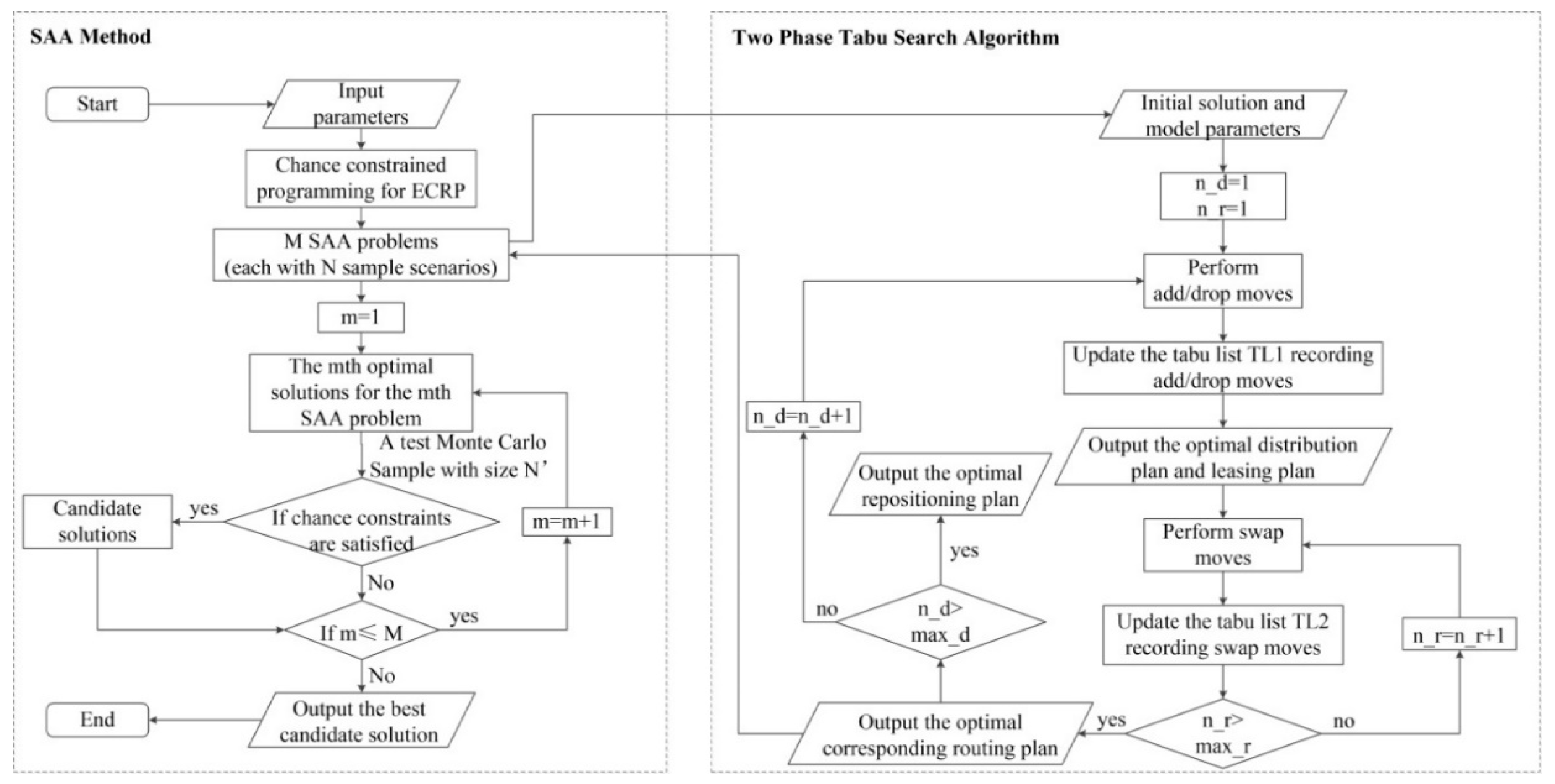
3. Solution Methodology
3.1. SAA Method
3.2. Two-Phase Tabu Search Algorithm
3.2.1. Distribution Phase
3.2.2. Routing Phase
4. Computational Study
4.1. Deterministic Case
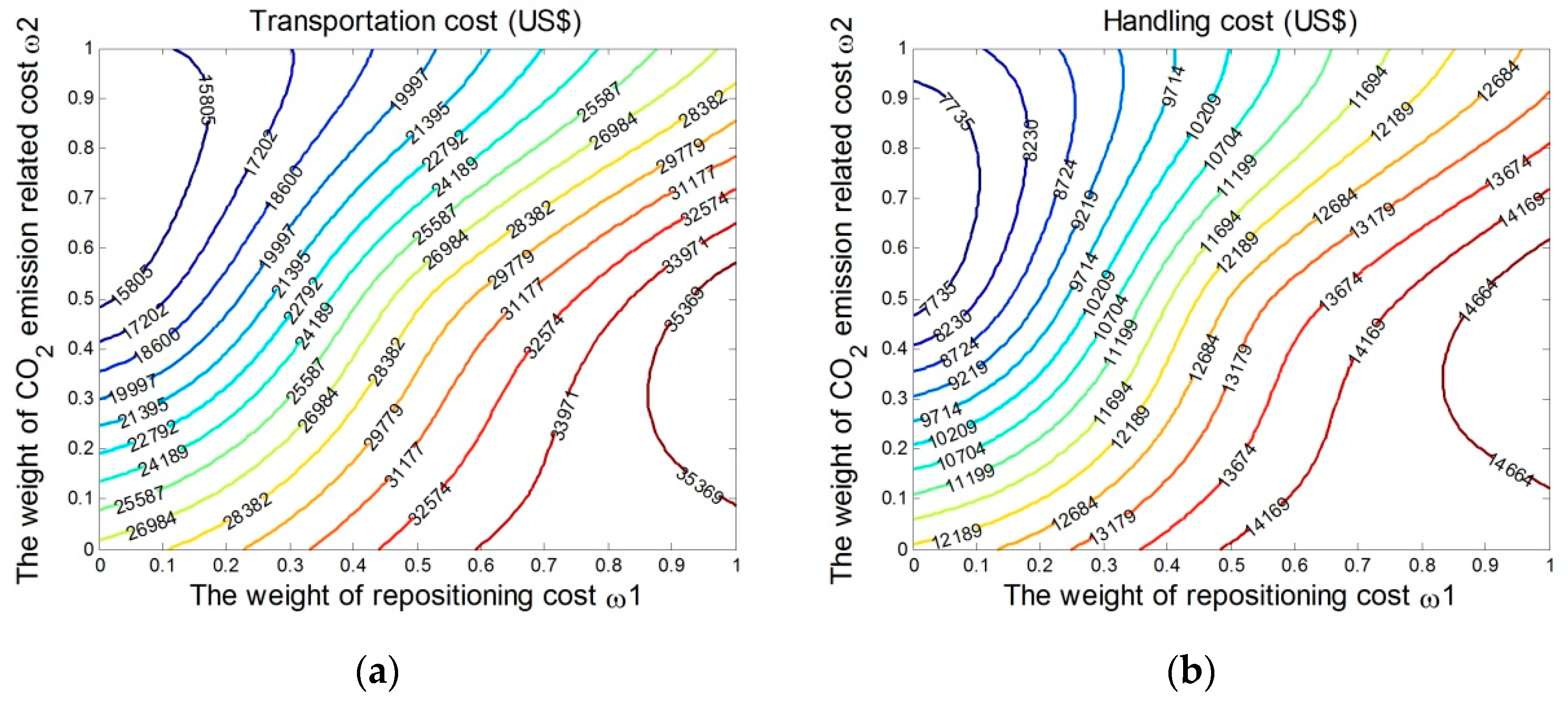
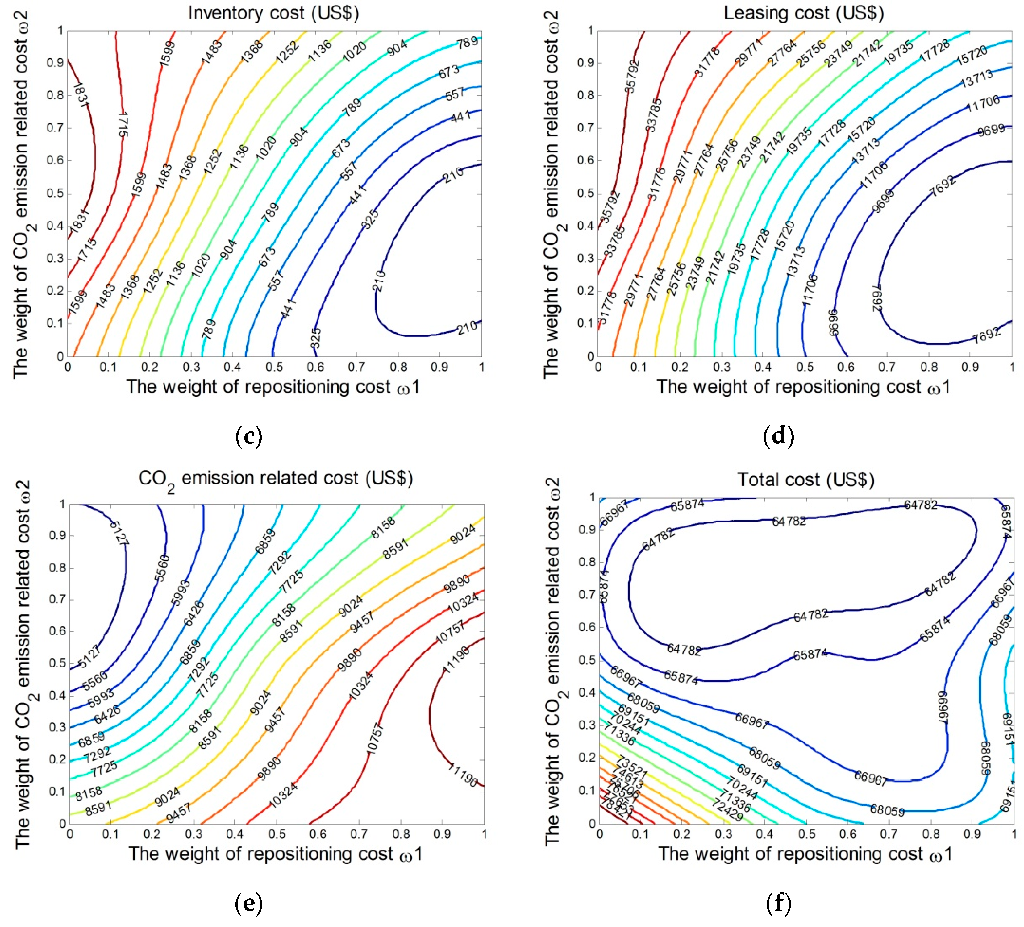
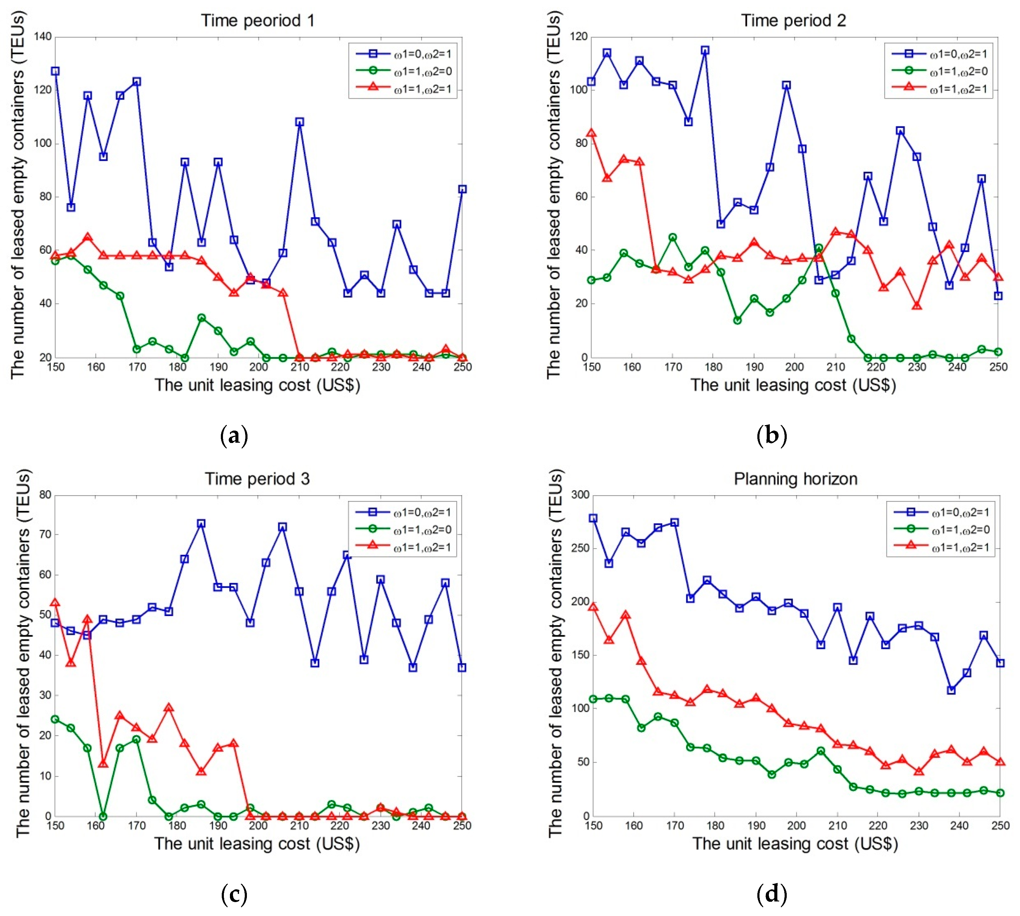
4.2. Stochastic Case
5. Conclusions
Author Contributions
Funding
Acknowledgments
Conflicts of Interest
References
- Zhao, Y.; Liu, R.; Zhang, X.; Whiteing, A. A chance-constrained stochastic approach to intermodal container routing problems. PLoS ONE 2018, 13, e0192275. [Google Scholar] [CrossRef] [PubMed]
- Long, Y.; Lee, L.H.; Chew, E.P. The sample average approximation method for empty container repositioning with uncertainties. Eur. J. Oper. Res. 2012, 222, 65–75. [Google Scholar] [CrossRef]
- Review of Maritime Transportation 2017. UNCTAD 2017. Available online: https://unctad.org/en/PublicationsLibrary/rmt2017_en.pdf (accessed on 15 October 2018).
- Demir, E.; Burgholzer, W.; Hrušovský, M.; Arıkan, E.; Jammernegg, W.; van Woensel, T. A green intermodal service network design problem with travel time uncertainty. Transp. Res. Part B Methodol. 2016, 93, 789–807. [Google Scholar] [CrossRef]
- Wang, Y.; Yan, X.; Zhou, Y.; Xue, Q.; Sun, L. Individuals’ acceptance to free-floating electric carsharing mode: A web-based survey in China. Int. J. Environ. Res. Public Health 2017, 14, 476. [Google Scholar] [CrossRef] [PubMed]
- Third IMO GHG Study 2014: Executive Summary and Final Report. International Maritime Organization 2014. Available online: http://www.imo.org/en/OurWork/Environment/PollutionPrevention/AirPollution/Documents/Third%20Greenhouse%20Gas%20Study/GHG3%20Executive%20Summary%20and%20Report.pdf (accessed on 15 October 2018).
- Huang, Y.F.; Hu, J.K.; Yang, B. Liner services network design and fleet deployment with empty container repositioning. Comput. Ind. Eng. 2015, 89, 116–124. [Google Scholar] [CrossRef]
- Jula, H.; Chassiakos, A.; Ioannou, P. Port dynamic empty container reuse. Transp. Res. Part E Logist. Transp. Rev. 2006, 42, 43–60. [Google Scholar] [CrossRef]
- Feng, C.M.; Chang, C.H. Empty container reposition planning for intra-Asia liner shipping. Marit. Policy Manag. 2008, 35, 469–489. [Google Scholar] [CrossRef]
- Braekers, K.; Janssens, G.K.; Caris, A. Challenges in managing empty container movements at multiple planning levels. Transp. Rev. 2011, 31, 681–708. [Google Scholar] [CrossRef]
- Song, D.P.; Dong, J.X. Empty container repositioning. In Handbook of Ocean Container Transport Logistics; Lee, C.Y., Meng, Q., Eds.; Springer: Cham, Switzerland, 2015; pp. 163–208. ISBN 978-3-319-11890-1. [Google Scholar]
- Florez, H. Empty-container Repositioning and Leasing: An Optimization Model. Ph.D. Thesis, Polytechnic-Institute of New York, Brooklyn, NY, USA, 1986. [Google Scholar]
- Crainic, T.G.; Delorme, L. Dual-ascent procedures for multicommodity location-allocation problems with balancing requirements. Transp. Sci. 1993, 27, 90–101. [Google Scholar] [CrossRef]
- Shintani, K.; Imai, A.; Nishimura, E.; Papadimitriou, S. The container shipping network design problem with empty container repositioning. Transp. Res. Part E Logist. Transp. Rev. 2007, 43, 39–59. [Google Scholar] [CrossRef]
- Song, D.P.; Carter, J. Empty container repositioning in liner shipping. Marit. Policy Manag. 2009, 36, 291–307. [Google Scholar] [CrossRef]
- Moon, I.K.; Do Ngoc, A.D.; Hur, Y.S. Positioning empty containers among multiple ports with leasing and purchasing considerations. OR Spectr. 2010, 32, 765–786. [Google Scholar] [CrossRef]
- Brouer, B.D.; Pisinger, D.; Spoorendonk, S. Liner shipping cargo allocation with repositioning of empty containers. INFOR: Inf. Syst. Oper. Res. 2011, 49, 109–124. [Google Scholar] [CrossRef]
- Meng, Q.; Wang, S. Liner shipping service network design with empty container repositioning. Transp. Res. Part E Logist. Transp. Rev. 2011, 47, 695–708. [Google Scholar] [CrossRef]
- Song, D.P.; Dong, J.X. Cargo routing and empty container repositioning in multiple shipping service routes. Transp. Res. Part B Methodol. 2012, 46, 1556–1575. [Google Scholar] [CrossRef]
- Song, D.P.; Dong, J.X. Long-haul liner service route design with ship deployment and empty container repositioning. Transp. Res. Part B Methodol. 2013, 55, 188–211. [Google Scholar] [CrossRef]
- An, F.; Hu, H.; Xie, C. Service network design in inland waterway liner transportation with empty container repositioning. Eur. Transp. Res. Rev. 2015, 7, 9. [Google Scholar] [CrossRef]
- Cheung, R.K.; Chen, C.Y. A two-stage stochastic network model and solution methods for the dynamic empty container allocation problem. Transp. Sci. 1998, 32, 142–162. [Google Scholar] [CrossRef]
- Crainic, T.G.; Gendreau, M.; Dejax, P. Dynamic and stochastic models for the allocation of empty containers. Oper. Res. 1993, 41, 102–126. [Google Scholar] [CrossRef]
- Li, J.A.; Liu, K.; Leung, S.C.; Lai, K.K. Empty container management in a port with long-run average criterion. Math. Comput. Model. 2004, 40, 85–100. [Google Scholar] [CrossRef]
- Li, J.A.; Leung, S.C.; Wu, Y.; Liu, K. Allocation of empty containers between multi-ports. Eur. J. Oper. Res. 2007, 182, 400–412. [Google Scholar] [CrossRef]
- Song, D.P. Characterizing optimal empty container reposition policy in periodic-review shuttle service systems. J. Oper. Res. Soc. 2007, 58, 122–133. [Google Scholar] [CrossRef]
- Lam, S.W.; Lee, L.H.; Tang, L.C. An approximate dynamic programming approach for the empty container allocation problem. Transp. Res. Part C Emerg. Technol. 2007, 15, 265–277. [Google Scholar] [CrossRef]
- Song, D.P.; Dong, J.X. Empty container management in cyclic shipping routes. Marit. Econ. Logist. 2008, 10, 335–361. [Google Scholar] [CrossRef]
- Di Francesco, M.; Crainic, T.G.; Zuddas, P. The effect of multi-scenario policies on empty container repositioning. Transp. Res. Part E Logist. Transp. Rev. 2009, 45, 758–770. [Google Scholar] [CrossRef]
- Song, D.P.; Zhang, Q. A fluid flow model for empty container repositioning policy with a single port and stochastic demand. SIAM J. Control Optim. 2010, 48, 3623–3642. [Google Scholar] [CrossRef]
- Song, D.P.; Dong, J.X. Flow balancing-based empty container repositioning in typical shipping service routes. Marit. Econ. Logist. 2011, 13, 61–77. [Google Scholar] [CrossRef]
- Lee, L.H.; Chew, E.P.; Luo, Y. Empty container management in multi-port system with inventory-based control. Int. J. Adv. Syst. Meas. 2012, 5, 164–177. [Google Scholar]
- Dong, J.X.; Xu, J.; Song, D.P. Assessment of empty container repositioning policies in maritime transport. Int. J. Logist. Manag. 2013, 24, 49–72. [Google Scholar] [CrossRef]
- Sainz Bernat, N.; Schulte, F.; Voß, S.; Böse, J. Empty container management at ports considering pollution, repair options, and street-turns. Math. Probl. Eng. 2016. [Google Scholar] [CrossRef]
- Choong, S.T.; Cole, M.H.; Kutanoglu, E. Empty container management for intermodal transportation networks. Transp. Res. Part E Logist. Transp. Rev. 2002, 38, 423–438. [Google Scholar] [CrossRef]
- Meng, Q.; Wang, S.; Liu, Z. Network design for shipping service of large-scale intermodal liners. Transp. Res. Rec. 2012, 2269, 42–50. [Google Scholar] [CrossRef]
- Braekers, K.; Caris, A.; Janssens, G.K. Optimal shipping routes and vessel size for intermodal barge transport with empty container repositioning. Comput. Ind. 2013, 64, 155–164. [Google Scholar] [CrossRef]
- Kolar, P.; Schramm, H.J.; Prockl, G. Intermodal transport and repositioning of empty containers in Central and Eastern Europe hinterland. J. Transp. Geogr. 2018, 69, 73–82. [Google Scholar] [CrossRef]
- Dong, J.X.; Song, D.P. Quantifying the impact of inland transport times on container fleet sizing in liner shipping services with uncertainties. OR Spectr. 2012, 34, 155–180. [Google Scholar] [CrossRef]
- Xie, Y.; Liang, X.; Ma, L.; Yan, H. Empty container management and coordination in intermodal transport. Eur. J. Oper. Res. 2017, 257, 223–232. [Google Scholar] [CrossRef]
- Song, D.P.; Xu, J. An operational activity-based method to estimate CO2 emissions from container shipping considering empty container repositioning. Transp. Res. Part D Transp. Environ. 2012, 17, 91–96. [Google Scholar] [CrossRef]
- Charnes, A.; Cooper, W.W. Chance-constrained programming. Manag. Sci. 1959, 6, 73–79. [Google Scholar] [CrossRef]
- Kleywegt, A.J.; Shapiro, A.; Homem-de-Mello, T. The sample average approximation method for stochastic discrete optimization. SIAM J. Optim. 2002, 12, 479–502. [Google Scholar] [CrossRef]
- Verweij, B.; Ahmed, S.; Kleywegt, A.J.; Nemhauser, G.; Shapiro, A. The sample average approximation method applied to stochastic routing problems: A computational study. Comput. Optim. Appl. 2003, 24, 289–333. [Google Scholar] [CrossRef]
- Pagnoncelli, B.K.; Ahmed, S.; Shapiro, A. Sample average approximation method for chance constrained programming: Theory and applications. J. Optim. Theory Appl. 2009, 142, 399–416. [Google Scholar] [CrossRef]
- Luedtke, J.; Ahmed, S. A sample approximation approach for optimization with probabilistic constraints. SIAM J. Optim. 2008, 19, 674–699. [Google Scholar] [CrossRef]
- Cao, Z.; Yuan, Z.; Zhang, S. Performance analysis of stop-skipping scheduling plans in rail transit under time-dependent demand. Int. J. Environ. Res. Public Health 2016, 13, 707. [Google Scholar] [CrossRef] [PubMed]
- Shen, L.; Tao, F.; Wang, S. Multi-Depot Open Vehicle Routing Problem with Time Windows Based on Carbon Trading. Int. J. Environ. Res. Public Health 2018, 15, 2025. [Google Scholar] [CrossRef] [PubMed]
- Crainic, T.G.; Gendreau, M.; Soriano, P.; Toulouse, M. A tabu search procedure for multicommodity location/allocation with balancing requirements. Ann. Oper. Res. 1993, 41, 359–383. [Google Scholar] [CrossRef]
- Pedersen, M.B.; Crainic, T.G.; Madsen, O.B. Models and tabu search metaheuristics for service network design with asset-balance requirements. Transp. Sci. 2009, 43, 158–177. [Google Scholar] [CrossRef]
- Sun, M.; Aronson, J.E.; McKeown, P.G.; Drinka, D. A tabu search heuristic procedure for the fixed charge transportation problem. Eur. J. Oper. Res. 1998, 106, 441–456. [Google Scholar] [CrossRef]


| Transportation Mode | Stochastic Demand and/or Supply | CO2 Emissions | Key References |
|---|---|---|---|
| Unimodal | No | No | Huang et al. [7]; Jula et al. [8]; Feng and Chang [9]; Florez [12]; Crainic and Delorme [13]; Shintani et al. [14]; Song and Carter [15]; Moon et al. [16]; Brouer et al. [17]; Meng and Wang [18]; Song and Dong [19,20]; An et al. [21] |
| Unimodal | Yes | No | Long et al. [2]; Cheung and Chen [22]; Crainic et al. [23]; Li et al. [24]; Li et al. [25]; Song [26]; Lam et al. [27]; Song and Dong [28]; Francesco et al. [29]; Song and Zhang [30]; Song and Dong [31]; Lee et al. [32]; Dong et al. [33] |
| Unimodal | Yes | Yes | Bernat et al. [34] |
| Intermodal | No | No | Choong et al. [35]; Meng et al. [36]; Braekers et al. [37]; Kolar et al. [38] |
| Intermodal | Yes | No | Dong and Song [39]; Xie et al. [40] |
| Intermodal | Yes | Yes | This paper |
| Term | Definition |
|---|---|
| Index and set | |
| the set of nodes, | |
| the set of railway stations | |
| the set of ports | |
| the set of railway stations with surplus empty containers, | |
| the set of railway stations with deficit empty containers, | |
| the set of ports with surplus empty containers, | |
| the set of ports with deficit empty containers, | |
| the set of arcs, | |
| the set of railway arcs, including the arcs between two railway stations and the arcs between one railway station and one port | |
| the set of ship arcs, i.e., the arcs between two ports | |
| the sets of candidate railway routes between two railway stations and from one railway station to one port, distinguished by the origin stations, destination railway stations/ports, and intermediate railway stations. | |
| the set of candidate ship routes distinguished by their port calling sequences | |
| the planning horizon | |
| two railway stations, | |
| two ports, | |
| a transportation arc, | |
| a candidate railway route, | |
| a candidate ship route, | |
| a time period, | |
| Input parameters | |
| the distance of arc a (km) | |
| the unit transportation cost of one empty container on railway arc a, (US$/TEU) | |
| the unit transportation cost of one empty container on ship arc a of ship route r (US$/TEU) | |
| the unit loading cost of one empty container at railway station i (US$/TEU) | |
| the unit unloading cost of one empty container at railway station j (US$/TEU) | |
| the unit loading cost of one empty container at port p (US$/TEU) | |
| the unit unloading cost of one empty container at port q (US$/TEU) | |
| the unit inventory cost of storing one empty container per time period at railway station i (US$/TEU) | |
| the unit inventory cost of storing one empty container per time period at port p (US$/TEU) | |
| the unit leasing cost of one empty container at railway station i (US$/TEU) | |
| the unit leasing cost of one empty container at port p (US$/TEU) | |
| the unit CO2 emission-related cost (US$/kg) | |
| the CO2 emissions of arc a (kg/TEU) | |
| the transportation capacity of railway arc a (TEUs) | |
| the transportation capacity of ship route r when one ship is deployed (TEUs) | |
| the handling capacity of railway station i, including loading and unloading operations (TEUs) | |
| the handling capacity of port p, including loading and unloading operations (TEUs) | |
| the inventory capacity of railway station i (TEUs) | |
| the inventory capacity of port p (TEUs) | |
| the number of empty containers stored at railway station i at the end of time t (TEUs) | |
| the number of empty containers stored at port p at the end of time t (TEUs) | |
| a binary variable, equal to 1 if the arc a is on the railway route k; 0 otherwise | |
| a binary variable, equal to 1 if the arc a is on the ship route r; 0 otherwise | |
| Random variables | |
| the uncertain demand of empty containers at railway station i at time t (TEUs) | |
| the uncertain supply of empty containers at railway station i at time t (TEUs) | |
| the uncertain demand of empty containers at port p at time t (TEUs) | |
| the uncertain supply of empty containers at port p at time t (TEUs) | |
| Decision variables | |
| the number of repositioned empty containers by train from i to j at time t | |
| the number of repositioned empty containers by ship from p to q at time t | |
| the number of repositioned empty containers by train from i to q at time t | |
| a binary variable, equal to 1 if railway route k is selected to transport empty containers from i to j at time t; 0 otherwise | |
| a binary variable, equal to 1 if ship route r is selected to transport empty containers from p to q at time t; 0 otherwise | |
| a binary variable, equal to 1 if railway route k is selected to transport empty containers from i to q at time t; 0 otherwise | |
| the number of leased empty containers at railway station i at time t | |
| the number of leased empty containers at port p at time t | |
| the vector of all decision variables at time t, i.e., |
| Arc | Distance (km) | Cost (US$/TEU) | CO2 (kg/TEU) |
|---|---|---|---|
| (S1, S2) | 195 | 59.25 | 9.86 |
| (S1, S4) | 158 | 53.7 | 7.99 |
| (S1, S5) | 158 | 53.7 | 7.99 |
| (S2, S3) | 190 | 58.5 | 9.61 |
| (S2, S6) | 98 | 44.7 | 5 |
| (S3, S7) | 88 | 43.2 | 4.45 |
| (S4, S5) | 145 | 51.75 | 7.34 |
| (S4, P1) | 135 | 50.25 | 6.83 |
| (S5, S6) | 100 | 45 | 5.06 |
| (S5, P1) | 165 | 54.75 | 8.35 |
| (S6, S7) | 100 | 45 | 5.06 |
| (S6, P2) | 100 | 45 | 5.06 |
| (S7, P3) | 100 | 45 | 5.06 |
| Ship Route | Port Calling Sequence | Arc | Cost (US$/TEU) | CO2 (kg/TEU) |
|---|---|---|---|---|
| 1 | P1→P2→P1 | (P1, P2) | 18 | 9.75 |
| 2 | P2→P3→P2 | (P2, P3) | 15 | 3.68 |
| 3 | P1→P3→P1 | (P1, P3) | 30 | 13.43 |
| 4 | P1→P2→P3→P2→P1 | (P1, P2) | 17 | 9.75 |
| (P2, P3) | 16 | 3.68 |
| Demand of Empty Containers (TEUs) | S1 | S2 | S3 | P1 | P2 | P3 |
|---|---|---|---|---|---|---|
| t = 1 | 424 | 428 | 392 | 490 | 446 | 632 |
| t = 2 | 396 | 324 | 414 | 530 | 548 | 454 |
| t = 3 | 378 | 292 | 406 | 582 | 532 | 594 |
| Supply of Empty Containers (TEUs) | S1 | S2 | S3 | P1 | P2 | P3 |
|---|---|---|---|---|---|---|
| t = 1 | 366 | 368 | 436 | 464 | 552 | 606 |
| t = 2 | 436 | 276 | 316 | 622 | 466 | 550 |
| t = 3 | 336 | 328 | 356 | 628 | 586 | 550 |
| Time Period t | Distribution Plan | Routing Plan | Leasing Plan |
|---|---|---|---|
| 1 | S3→S1: 10 TEUs | S3→S2→S1 | S1: 48 TEUs |
| S3→S2: 34 TEUs | S3→S2 | ||
| P2→S2: 26 TEUs | P2→S6→S2 | ||
| P2→P1: 26 TEUs | Ship route 4 | ||
| P2→P3: 26 TEUs | Ship route 2 | ||
| 2 | S1→S2: 20 TEUs | S1→S2 | S2: 18 TEUs S3: 22 TEUs |
| S1→S3: 20 TEUs | S1→S2→S3 | ||
| P1→P2: 24 TEUs | Ship route 4 | ||
| P3→S2: 10 TEUs | P3→S7→S6→S2 | ||
| P3→S3: 56 TEUs | P3→S7→S3 | ||
| P3→P2: 30 TEUs | Ship route 2 | ||
| 3 | S2→S3: 36 TEUs | S2→S3 | - |
| P1→S1: 42 TEUs | P1→S4→S1 | ||
| P1→P3: 22 TEUs | Ship route 3 | ||
| P2→S3: 14 TEUs | P2→S6→S7→S3 | ||
| P2→P3: 22 TEUs | Ship route 2 |
| Time Period t | Transportation Cost (US$) | Handling Cost (US$) | Inventory Cost (US$) | Leasing Cost (US$) | CO2 Emission-Related Cost (US$) | Total Cost (US$) |
|---|---|---|---|---|---|---|
| 1 | 6330.7 | 3600 | 156.8 | 9600 | 2264.4 | 22,012 |
| 2 | 10,684 | 4800 | 380.8 | 8000 | 3229.5 | 27,095 |
| 3 | 9326.7 | 4080 | 380.8 | 0 | 3097.6 | 16,885 |
| Total | 26,342 | 12,540 | 918.4 | 17,600 | 8591.5 | 65,991 |
| Time Period t | Distribution Plan | Routing Plan | Leasing Plan |
|---|---|---|---|
| 1 | S3→S1: 16 TEUs | S3→S2→S1 | S1: 48 TEUs S2: 3 TEUs |
| S3→S2: 27 TEUs | S3→S2 | ||
| P2→S2: 36 TEUs | P2→S6→S2 | ||
| P2→P1: 32 TEUs | Ship route 4 | ||
| P2→P3: 32 TEUs | Ship route 2 | ||
| 2 | S1→S2: 24 TEUs | S1→S2 | S2: 22 TEUs S3: 26 TEUs |
| S1→S3: 21 TEUs | S1→S2→S3 | ||
| P1→P2: 56 TEUs | Ship route 4 | ||
| P3→S2: 8 TEUs | P3→S7→S6→S2 | ||
| P3→S3: 62 TEUs | P3→S7→S3 | ||
| P3→P2: 32 TEUs | Ship route 2 | ||
| 3 | S2→S1: 16 TEUs | S2→S1 | S1: 2 TEUs S3: 5 TEUs |
| S2→S3: 30 TEUs | S2→S3 | ||
| P1→S1: 41 TEUs | P1→S4→S1 | ||
| P1→P3: 32 TEUs | Ship route 3 | ||
| P2→S3: 21 TEUs | P2→S6→S7→S3 | ||
| P2→P3: 30 TEUs | Ship route 2 |
| Time Period t | Transportation Cost (US$) | Handling Cost (US$) | Inventory Cost (US$) | Leasing Cost (US$) | CO2 Emission-Related Cost (US$) | Total Cost (US$) |
|---|---|---|---|---|---|---|
| 1 | 7716.7 | 4290 | 177.1 | 10,200 | 2725.8 | 25,110 |
| 2 | 11,873 | 6090 | 459.3 | 9600 | 4039.7 | 32,062 |
| 3 | 11,172 | 5100 | 503.4 | 1400 | 3799.6 | 21,975 |
| Total | 30,762 | 15,480 | 1139.8 | 21200 | 10,565 | 79,147 |
© 2018 by the authors. Licensee MDPI, Basel, Switzerland. This article is an open access article distributed under the terms and conditions of the Creative Commons Attribution (CC BY) license (http://creativecommons.org/licenses/by/4.0/).
Share and Cite
Zhao, Y.; Xue, Q.; Zhang, X. Stochastic Empty Container Repositioning Problem with CO2 Emission Considerations for an Intermodal Transportation System. Sustainability 2018, 10, 4211. https://doi.org/10.3390/su10114211
Zhao Y, Xue Q, Zhang X. Stochastic Empty Container Repositioning Problem with CO2 Emission Considerations for an Intermodal Transportation System. Sustainability. 2018; 10(11):4211. https://doi.org/10.3390/su10114211
Chicago/Turabian StyleZhao, Yi, Qingwan Xue, and Xi Zhang. 2018. "Stochastic Empty Container Repositioning Problem with CO2 Emission Considerations for an Intermodal Transportation System" Sustainability 10, no. 11: 4211. https://doi.org/10.3390/su10114211
APA StyleZhao, Y., Xue, Q., & Zhang, X. (2018). Stochastic Empty Container Repositioning Problem with CO2 Emission Considerations for an Intermodal Transportation System. Sustainability, 10(11), 4211. https://doi.org/10.3390/su10114211