Energy Consumption Optimization in Irrigation Networks Supplied by a Standalone Direct Pumping Photovoltaic System

Abstract

Due to the fact that irrigation networks are water and energy hungry and that both resources are scarce, many strategies have been developed to reduce this consumption. Solar energy sources have emerged as a green alternative with lower energy costs and, consequently, lower environmental impacts. In this work, a new methodology is proposed to select a scheduled program for irrigation which minimizes the number of photovoltaic solar panels to be installed and which better fits energy consumption (calculated for discrete potential combinations, assisted by programming software) to available energy obtained by panels without any power conditioning unit. Thus, the irrigation hours available to satisfy the water demands are limited by sunlight, the schedule type of irrigation has to be rigid (rotation predetermined), and the pressure at any node has to be above the minimum pressure required by standards. A case study was undertaken and, after running the software 10⁵ times, the best result was an irrigation schedule which satisfied all the requirements, involving the installation of 651 solar panels and energy consumption of 428.74 kWh per day, to deliver water to orchards of different varieties of citrus fruit spread over 167.7 ha.

1. Introduction

It bears no surprise that irrigation agriculture accounts for 70% of the world’s water use and that water and energy consumption are inextricably linked [1]. Given the future demands of food production, efficient management strategies for both resources are of paramount importance. Some of the proposals to improve water efficiency in irrigation networks are the use of pressurized water distribution networks and also the use of emitters (sprinklers or drip irrigation) [2].

From the design and management of water irrigation networks standpoint, the fact that sustainable management of pressurized networks has become the key objective for water irrigation managers is reflected by the high number of studies dealing with improvements in water efficiency [3,4,5], with recent approaches dealing with energy optimization, including: methods for the sectoring of irrigation networks [6]; changes in the operating system, from scheduled to on-demand irrigation [7]; selection of new pumping systems; and/or, changes in the diameter of water sprinklers [8], etc.

Thus, in regions where water is scarce [9,10], several technologies have been developed to reduce water and energy consumption. However, water and energy are so interdependent in pressurized irrigation networks, that in semi-arid regions energy needs have reached values as high as 0.95–1.55 kWh/m³ [11].

The high cost of diesel fuels and the deficit in electricity affects irrigation network managers’ decisions when considering the need to meet water and energy requirements for crop irrigation. Solar water pumping based on photovoltaic (PV) technology is one of the hottest topics in water irrigation networks because it has become an attractive alternative with proven economic viability [12,13]. Some other approaches are focused on calculating energy production from a PV [14] or obtaining maximum power from PV with minimum motor losses [15].

Solar photovoltaic technology consists of a PV array that provides electricity for driving the pumps. This direct couple system is composed of a PV generator (which converts the irradiance (W m⁻²) into direct current; DC), a frequency converter (which converts the DC into alternating current; AC) and an asynchronous motor (which converts AC into shaft work moving the pump) [16,17].

The key advantages of incorporating PV technology in the optimization problem consist of the reduction in the operating costs of pumping water into the system [18] and the associated environmental benefits [19]. However, the system should guarantee the supply for irrigating the crops and, as the hourly irradiance is an input in the optimization process, the location and the period of the year become important restrictions, as water needs are not the only parameter which controls the process.

In this new scenario, and considering the current state of the technology, this approach deals with the advantages of solar energy as a green alternative [12,14]; however, it deals with the problem as a new optimization irrigation schedule minimizing the number of PV panels to be installed while also minimizing the energy requirements of the system. Some previous research has already faced this problem without considering the synchronization between the energy available and the energy required by pumping devices [20]. Some other works [21,22] solve this synchronization problem by considering a fixed number of PV panels (and also the available energy). The key difference here with regard to previous approaches is that it has been analyzed as a multi-objective optimization algorithm (minimization of the number of PV panels and energy consumption).

In this approach, the number of segments is constant and the pressurized irrigation network has been modeled using open source hydraulic modeling software. The irrigation network should be adjusted to meet all the water demands (supplying every consumption node with a pressure above the minimum required pressure). The methodology presented here calculates the most efficient combination of areas irrigated simultaneously, which satisfies water demand in crops with pressures above the threshold service, with fewer PV panels installed and with lower energy consumption. In order to meet these requirements, the hourly energy consumption (by the irrigation network) should be as close as possible to the available energy, due to the hourly irradiance curve.

The water energy nexus (watergy) has become one of the hottest topics of the water industry. The relationship between water and energy has been calculated in pressurized networks including leakage [23,24]. Some other approaches have focused on the efficient operation of pumping systems [25,26], or on defining performance indicators to assess practitioners and decision-makers [23,27]. The same has happened with regard to irrigation networks, where this close relationship has been described [28], the joint benefits of water and energy savings have been calculated [29] and several case studies have been proposed focusing on the delivery scheduling method [7,8], pipeline rehabilitation [30] and even energy recovery [31].

As the optimization problem is very time-consuming (the values of energy savings at every time step period vary, daily sums of energy/water saved were calculated), and every hydraulic simulation for the possible combinations (rigid scheduled irrigation) were calculated using Matlab^® code to assist with the EPAnet toolkit [32]. In every combination, the energy audit in irrigation networks [29] was calculated using a Matlab-based graphical user interface (GUI; UAEnergy) developed for students and practitioners which can be downloaded at “http://rua.ua.es/dspace/handle/10045/76947”.

The paper is organized as follows: Section 2.1 shows the calculation of the net power transferred as hydraulic energy (Appendix A shows a way of calculating hourly irradiance); Section 2.2 shows the crop water demands; Section 2.3 presents the energy audits in irrigation networks; the schedule for irrigation is depicted in Section 2.4; and, the optimization problem is described in Section 3. A case study is presented in Section 4; where the energy requirements are shown in Section 4.2, the quantification of the number of PV panels is calculated in Section 4.3, the results of the energy audit for the best demand multiplier pattern (DPM) combinations are shown in Section 4.4 and, finally, a comparison between cases is depicted in Section 4.5.

2. Materials and Methods

In this section, some ideas about PV panels and the irrigation network are provided as background knowledge to the optimization problem. The calculation of the hourly distribution of irradiance for each month [33] is described here and in Appendix A. Water requirements and the scheduled irrigation program are calculated and added to a calibrated hydraulic simulation model. In this software, a segmentation is performed (in order to reach a constant injected flow rate which produces low head losses through the pipelines) and the energy audit should be calculated (in this work, the energy audit has been calculated using UAEnergy (Matlab-based educational software).

2.1. Net Power Transferred to the Water

The starting point should be to determine the hourly distribution of monthly solar radiation (also considering the optimum angle of inclination (β) of the photovoltaic panels).

The net photovoltaic power provided by a PV generator is calculated as follows:

$$P_{PV}=\{\begin{array}{cc}\frac{I\left(t\right)}{I_{STC}}PP\left(1-\gamma \left(T_{cell}-T_{STC}\right)\right)& if I\left(t\right)>I_m\\ 0& if I\left(t\right)<I_m\end{array}$$

(1)

where $P_{PV}$ is the power obtained directly by the photovoltaic system, $I(t)$ is the irradiance on the inclined collector plane expressed in W m⁻², $I_{STC}$ is the irradiance under standard conditions (1000 W m⁻²), PP is the peak power generated by the PV modules (in W), $\gamma$ is the performance decay coefficient due to the rising temperature of the cell, $T_{cell}$ is the cell temperature in the module and $T_{STC}$ is the cell temperature under standard test conditions (25 °C). It will be necessary to determine the minimum irradiation ($I_m$), the threshold value (depending on the frequency inverter and also the PV peak power) which may range between 250–500 W m⁻² [34,35]. This value represents the daily irrigation period (i.e., the number of hours of irrigation).

The net power that it is finally transferred to water is calculated, considering the efficiency of the devices involved in the process:

$$P_h={\eta }_p{\eta }_{am}{\eta }_{fc}{P}_{PV}$$

(2)

where $P_h$ is the shaft power transferred to water, $P_{PV}$ is the power obtained directly by the photovoltaic system, and ${\eta }_p$, ${\eta }_{am}$ and ${\eta }_{fc}$ are the pump, asynchronous motor and converter efficiency (-), respectively.

2.2. Water Demands and Network Sectoring

When decision-makers are dealing with the reduction of energy consumption in irrigation networks, the first step is to properly calculate the amount of water required by crops.

Several approaches for calculating crop water needs have been proposed. Among them, the most widely used is the Penman-Monteith FAO method [36] which considers the reference evapotranspiration (ET_o) and the type of crop, characterized by the crop coefficient (K_c). This method is robust and valid, both for the irrigation network design stage and for selecting the irrigation program schedule (once the crops are growing). Some other methods, which calculate water requirements more accurately, are based on direct measurements of the soil water content or on plant water stress monitoring [37,38]. Their use would require physically having the irrigation network working, as sensors would need to be in place to obtain the data required (in other words, these methods can only be properly used in the irrigation schedule programming stage).

From the design and management of water irrigation networks standpoint, and given the water needs of every irrigation area, the circulating flows and the irrigation time are calculated for every hydrant and/or subunit in the water irrigation network. These outlet hydrant demands depend on the type of emitters, the irrigated area, application efficiency, etc. and their value is constant for every subunit, while irrigation time depends on the crop needs and the scheduling program of irrigation. In this new approach, the minimum irradiation ($I_m$), from which the solar power can be obtained from the panels reveals the start time and the number of hours of irrigation. The pressure level at every hydrant is another parameter to check and depends on the features of the irrigation subunits (lateral and submain pipe sizes, emitter type, slope, etc) [39]. Clearly, pressurized irrigation requires an energy input (frequently a pump device is using to introduce shaft work into the system) to satisfy the water demands by delivering water at pressure levels over the minimum pressure required by standards.

All this information, and also the pipe and hydrant characteristics needs to be added to a model in hydraulic simulation software (EPANET or any other) to solve the hydraulic problem. First, the model should be calibrated to represent reality. The objective of the calibration is to observe a good response between the simulated (model predicted) and the observed values (pressures and flows at several points of the network) over the entire simulation period. A model provides the user with knowledge of pressure levels in consumption nodes, flows, head losses and velocities in pipes, to simulate the energy requirements, etc. In short, it returns valuable information required in decision-making processes.

2.3. Energy Audit in Irrigation Networks

The required shaft work in pumps (at every moment of the day) is calculated with the energy audit in irrigation networks [29]. The energy balance (where $t_p$ is the simulation period) results in Equation (3):

$$E_{input}\left(t_p\right)=E_n\left(t_p\right)+E_p\left(t_p\right)\pm ∆E_c\left(t_p\right)=E_u\left(t_p\right)+E_l\left(t_p\right)+E_f\left(t_p\right)+E_v\left(t_p\right)$$

(3)

where E_n($t_p$) is the energy supplied by reservoirs, E_p$\left(t_p\right)$ is the energy supplied by pumps, E_u$\left(t_p\right)$ is the energy delivered to the crops (through the water supplied), E_l$\left(t_p\right)$ is the energy lost through water losses, E_f$\left(t_p\right)$ is the energy dissipated by friction in pipes, E_v$\left(t_p\right)$ is the energy dissipated in valves, and ΔE_c$\left(t_p\right)$ is the energy that can be stored in a compensation tank which accumulates water during low consumption hours and releases it in peak hours.

2.4. Network Management

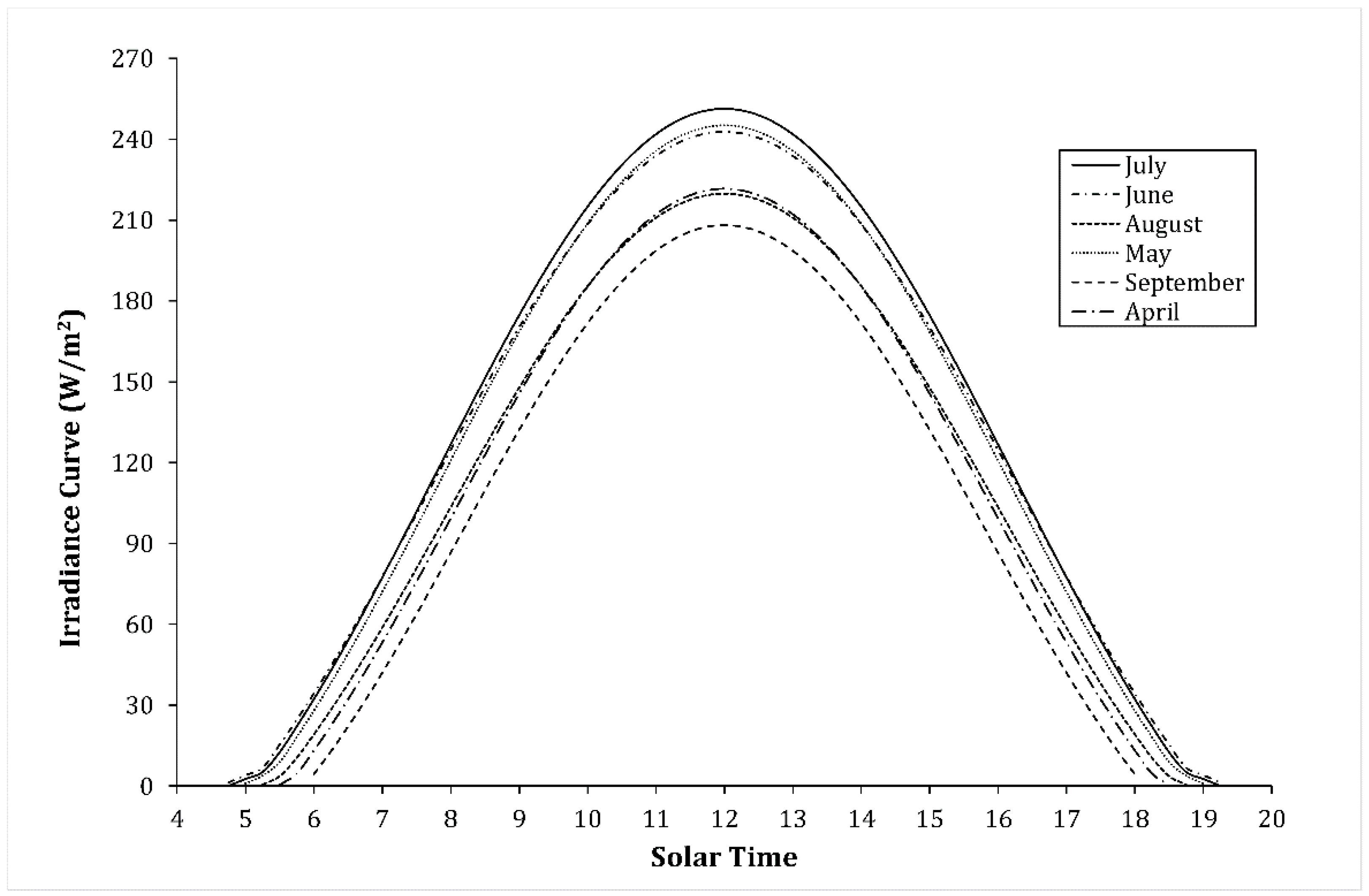
Once the model has been calibrated, the delivery scheduling method in an irrigation system demonstrates different levels of energy consumption [10,40]. These schedule types may be classified [41], in order of increasing flexibility, as rigid (rotation, predetermined), central control, intermediate control (arranged) or flexible (on-demand, modifiable). As the energy provided by the PV presents additional restrictions, such as a fixed time for irrigation, and also hourly and monthly energy availability variation (Figure 1), the consumption in segments with regard to time is the combination which involves energy consumption in pumps (shaft work) which best fits the available energy. The combinations of water demands have different values of energy consumption in pumps (E_p$\left(t_p\right)$) as some other parameters in the energy audit are also affected. To name a few, the relationship between energy dissipated by friction in pipes and flow is of a quadratic type, and the leakage depends (among some other factors) on the pressure levels (whose figures are directly linked to head losses and circulating flows along the network).

With these limitations, rigid rotation scheduled irrigation is the only irrigation type which allows network managers to fit the energy consumption to the energy available from the PV. Additionally, every subunit or hydrant (node where water leaves the irrigation network) is controlled by an electro valve (a common device in irrigation networks) which helps the practitioner to control irrigation.

3. Optimization Problem

3.1. Input Data

The input data required to calculate the most energy efficient combination are depicted here.

• Irradiance input data:

  ○

  β is the angle of inclination (radians) of the photovoltaic panels

  ○

  $I_{sc}$ is the solar constant (1367 W m⁻²)

  ○

  $I_{STC}$ is the irradiance under standard conditions (1000 W m⁻²)

  ○

  $d$ is the performance decay coefficient due to the rising temperature of the cell (0.004 °C⁻¹)

  ○

  H is the global irradiance on horizontal surface (kWh m⁻²)

  ○

  $T_{STC}$ is the cell temperature under standard test conditions (25 °C)

  ○

  $T_{avg}$ is the monthly average temperature (°C)

  ○

  φ is the latitude angle (positive to the North) (radians)

  ○

  n is the day of the representative month

  ○

  ρ is the albedo (-)

  ○

  PP is the peak power generated by the PV modules (W)

  ○

  ${\eta }_p$ is the pump efficiency (-).

  ○

  ${\eta }_{am}$ is the asynchronous motor efficiency (-).

  ○

  ${\eta }_{fc}$ is the converter efficiency (-).

• Hydraulic input data:

  ○

  A calibrated water-pressurized network which represents the water delivery in crops. This file must represent the hydraulic features of the system and no errors should appear when running this model. Moreover, the water requirements of the network should be defined in the model and the segments (if any) should also be included in the model.

  ○

  Report time step for the case study (minutes)

  ○

  ${\left(\frac{P}{\gamma }\right)}_{threshold}$ (defined in Section 2.2) is the minimum pressure required by standards at any hydrant and any time (m.w.c.)

  ○

  $T_{irr}$ (defined in Section 2.2) is the irrigation time (minutes).

  ○

  $T_{min\_irr}$ is the minimum irrigation time (minutes), a value which shows that if a node is delivering water to crops, it should be doing it for a time at least equal to or higher than this value.

3.2. Optimization Parameters

The optimization parameters for a discrete optimization problem (like the problem analyzed here) where the combinations are finite (although high in number) are the demand multiplier patterns (DPMs). Every network studied is divided into n regions and every region is assumed to follow the same diurnal curve (i.e., same set of DPMs), with a DPM being a group of values (row vector, size (1, x)) which consider variation in time of the consumption nodes’ base demands.

The pattern time step represents the time interval after which a change in time patterns is produced (1 h, 30 min, etc.), and the total simulation period is equal to the hours in which the irradiance curve is producing energy (7–9 h). In short, if the pattern time step is equal to 20 min, and the hours of simulation are 8 h, the DPM which analyses the evolution of irrigation in one segment has 480/20 = 24 values.

The network is divided into n segments (groups of subunits which totals the same base demand and create a constant value for the injected flow), each of them following their particular set of DPMs. So, each combination should be composed of a matrix of size (i, j) (i rows, one per sector; and j columns, one per every time step considered), with the following values:

$$a_{ij}=\{\begin{array}{ll} 1& if open\\ 0& if closed\end{array}$$

(4)

The values in these combinations are 1 (if subunit open) or 0 (if closed). The sum of the values per row should be equal to the irrigation time per sector (in short, if the crop requires 2 h of water and the time step is 30 min, there have to be four values which should be equal to 1).

The sum of the values per column of every combination should be less than or equal to the maximum number of segments which can be opened simultaneously. As the irrigation system is divided into n segments, the potential combination of n segments irrigating simultaneously should be calculated as follows:

$$N_{Poscomb}={\displaystyle \sum }_{i=1}^n\left(\begin{array}{c}n\\ i\end{array}\right)$$

(5)

where n = number of segments and i is the number of segments irrigating simultaneously.

Among these combinations, pressured deficit conditions eliminate some possibilities as the network is not ready to satisfy the water requirements with the pressure above the minimum pressure threshold.

Finally, as the electro-valves have to be opened for a time longer than the minimum irrigation time, there is one additional restriction. If there is a subunit opened (a 1 in the matrix), there have to be consecutive values up to a value of time with the subunit opened (i.e., if time step is 30 min, and minimum irrigation time is equal to one hour, there have to be at least two consecutive values equal to 1). This restriction has been adopted to reduce the number of valves opening and closing.

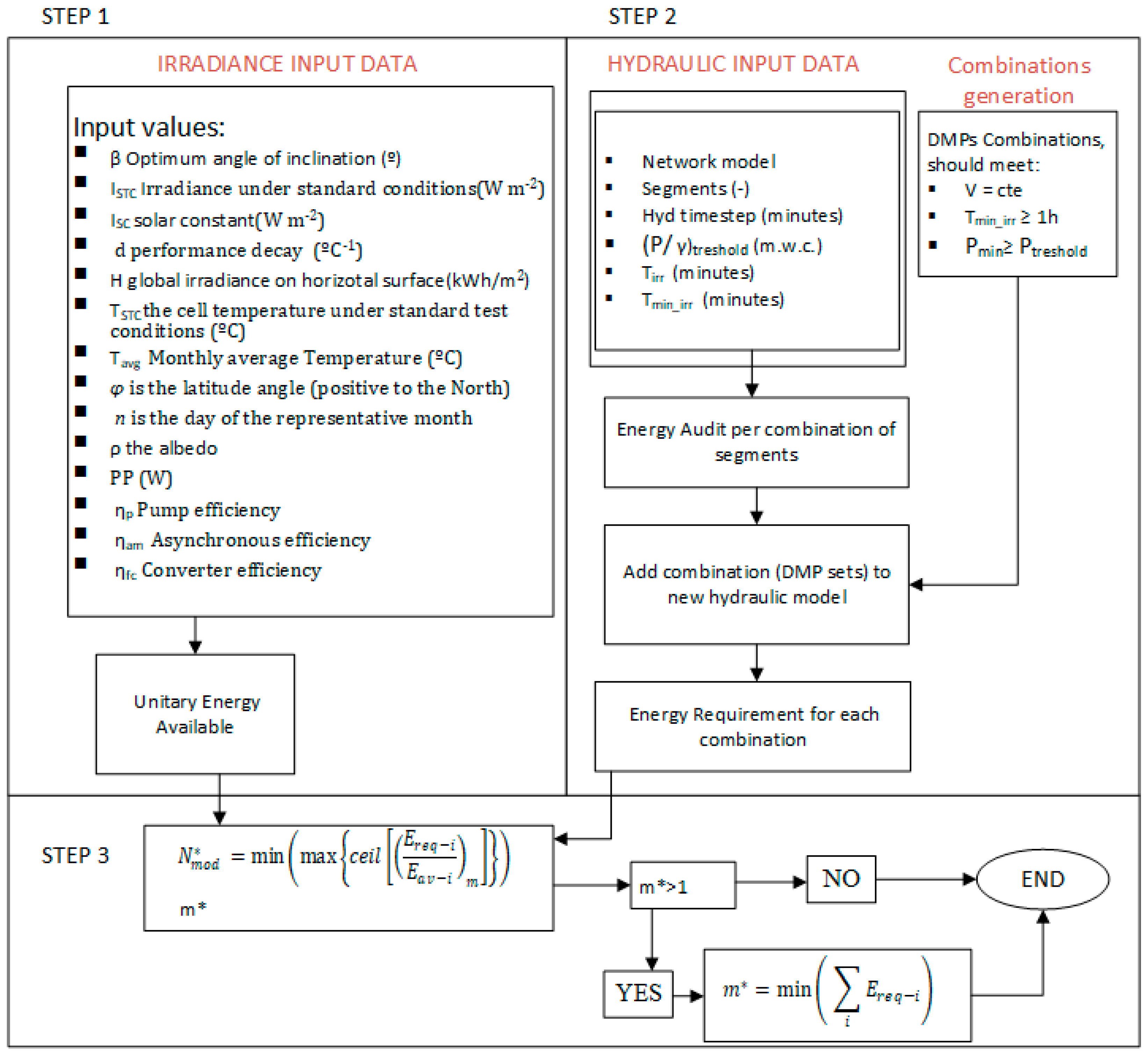
3.3. Calculation Process

Step 1

The first stage in the calculation is focused on calculating the monthly energy available per PV system. The unitary energy available is computed (Section 2.1, Appendix A).

Step 2

The second stage involves calculating the shaft work required by the pumps in the network (Section 2.3) for every segment combination Equation (5). Moreover, the m potential cases (DPMs) are calculated with the aforementioned restrictions:

• volume delivery should be constant
• the minimum pressure at every node and at every time should always be equal to or higher than the minimum pressure required by standards
• every time a segment is delivering water, the electro-valves have to be opened for a period longer than the minimum irrigation time.

For each of the m combinations, the DPMs are added to the initial irrigation network model (hydraulic input data) modifying their hydraulic response, which should be calculated with the use of hydraulic simulation software (as many combinations should be performed, programming software to assist with the hydraulic software is also recommended). The minimum pressure at every consumption node should be above the minimum threshold (if not, the DPM combination is rejected) and the hourly energy audit is also calculated.

Step 3

For the m combination, and at every i time step, the number of solar panels is calculated as:

$$N_{mod}^{\ast }=\min \left(\max \left\{ceil\left[{\left(\frac{E_{req-i}}{E_{av-i}}\right)}_m\right]\right\}\right)$$

(6)

where $E_{av-i}$ is the i-th value for the unitary energy available (calculated in Step 1) and $E_{req-i}$ is the i-th value for the energy available (calculated in Step 2). The quotient $ceil\left[{\left(\frac{E_{req-i}}{E_{av-i}}\right)}_m\right]$ represents the number of solar panels to satisfy the i-th water demand (“ceil” being the ceiling function that takes as input a real number X and gives as output the nearest integer greater than or equal X). The maximum of these i values results in the number of solar panels required for the m combination. Finally, a row vector of size (1, m) is obtained (one for each m combination) and the minimum of these figures should be the number of the modulus ($N_{mod}^{\ast }$) obtained at the m* combination.

If m* = 1, this should be the final DPM (minimizing the number of solar panels), but if there is more than one possible combination, the selected combination should be the one with lower energy required, as follows:

$$m^{\ast }=\min \left({\displaystyle \sum }_i{E}_{req-i}\right)$$

(7)

where ${{\displaystyle \sum }}_i{E}_{req-i}$ is the sum of the total energy required for the combinations with the lowest number of the modulus ($N_{mod}^{\ast }$).

The general flow-chart of this methodology is shown in Figure 2.

4. Numerical Example

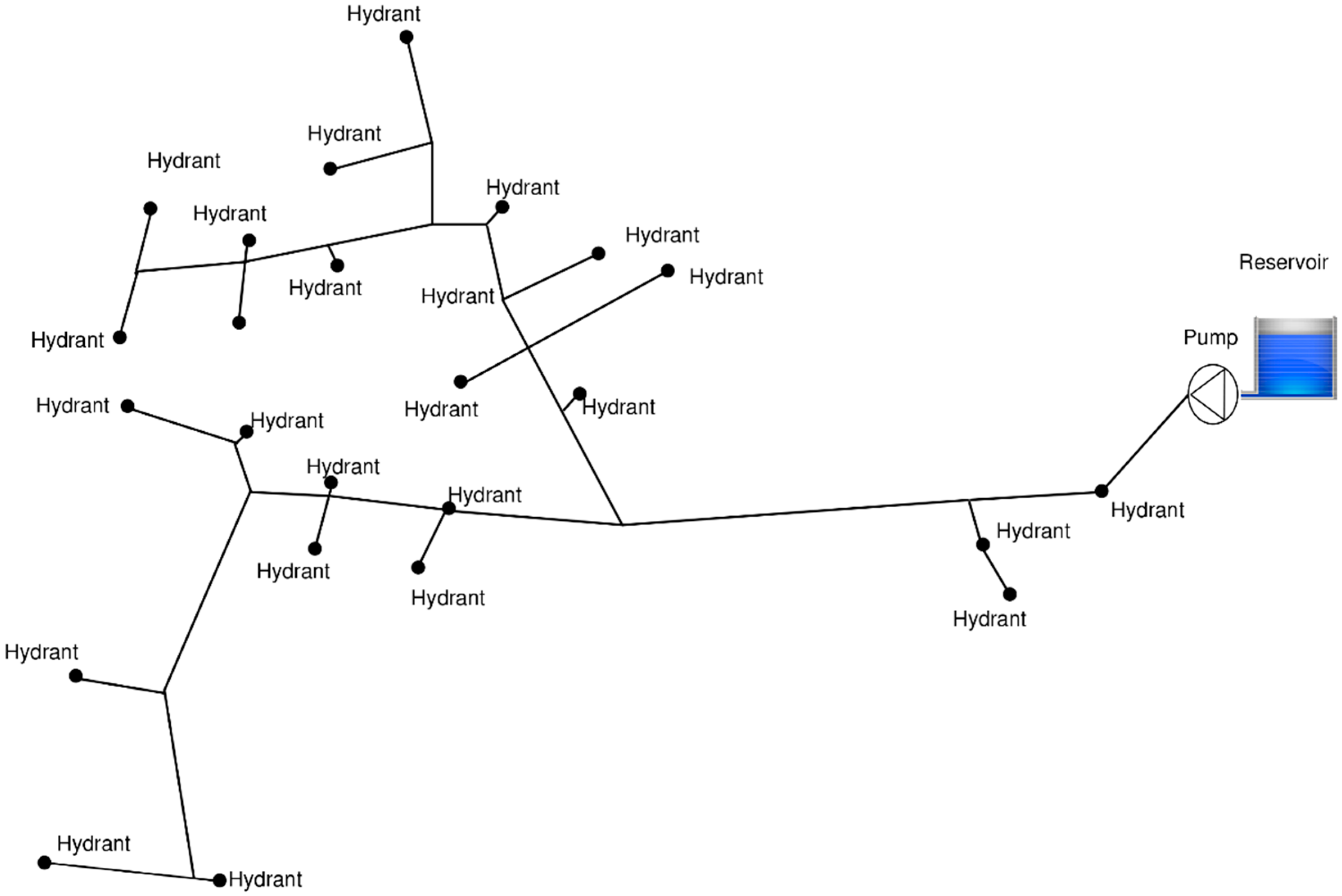
To illustrate the proposed methodology, a case study is presented here. Two scenarios are analyzed, Case 0 (current state), and Case 1 which entails direct pumping supplied by photovoltaic energy. The comparison was undertaken for the month with the highest water demands, July. Figure 3 shows a branched irrigation network (the Albamix network) in the western Mediterranean area of Spain. The data required to calculate irradiance curves are shown in

Table 1. Data required for irradiance curve calculation.

β = 15°	Havg = 8 kWh m−2	n = 198 (-)	${\eta }_{am}$ = 0.8 (-)
$I_{sc}$ = 1367 W m−2	$T_{STC}$ = 25 °C	ρ = 0.2 (-)	${\eta }_{fc}$ = 0.95 (-)
$I_{STC}$ = 1000 Wm−2	Tavg = 24.9 °C	PP = 250 W
d = 0.004 °C−1	φ = 39.47°	${\eta }_p$ = 0.75 (-)

. The Albamix network consists of 132 nodes and 131 pipes and supplies water to 167.7 ha to irrigate orchards containing different varieties of citrus fruit, with a usual planting pattern of 5 × 4 m² per tree. The total length of the network is 4.05 km. The pipe material is PVC, the pipe roughness for the aged pipes is 0.02 mm (a common value in water irrigation networks; [42]), and the minimum service pressure required is ${\left(\frac{P}{\gamma }\right)}_{threshold}$ = 25 m of water column. The irrigation networks were grouped into five segments which were determined based on the criterion of uniformity of pressure (and consequently flow) at each subunit. The water demands for the consumption of each segment were 79.7, 84.4, 85.4, 85.3 and 84 L/s for sectors 1, 2, 3, 4 and 5, respectively. All the subunits were equipped with drippers (4 L/h per emitter) and six emitters were required to irrigate every tree. The irrigation management system (current state; Case 0) is based on central system scheduled delivery and the total irrigation time ($T_{irr}$) varies with regard to every month considered. The monthly water demands were calculated with the meteorological information recovered in the irrigation area and the reference crop evapotranspiration was calculated using the Penman-Monteith method from the last 13 years (from 2005–2017). Regional recommendations [43] were followed to calibrate crop coefficients (K_c), and finally, the monthly average water needs varied from 0.31 L/m² in January to 3.4 L/m² in July. The irrigation time values are depicted in

Table 2. Monthly irrigation time (water demands) in the Albamix network.

Month	January	February	March	April	May	June
Irr. time (h)	0.52	0.69	1.12	1.29	1.93	2.92
Month	July	August	September	October	November	December
Irr. time (h)	3.25	2.70	1.62	0.75	0.43	0.30

.

The minimum irrigation time $\left(T_{\min \_irr}\right)$ is equal to 1 h (once the segment is opened, it has to be delivering water for at least 60 min), the time profitable to convert solar energy into shaft work in pumps is 9 h (540 min) and the report time step is 10 min, which means that there are 540/10 = 54 periods of time for every subunit to be opened or closed (six values hourly for 9 h). In July (the month with highest water requirements), every segment should be irrigated for 3.25 h/day (Table 2) and means that our five (one per sector) DPMs should consider an irrigation period of 200 min (20 periods out of these aforementioned 54 periods should consider the segment opened while 34 periods consider the segment closed).

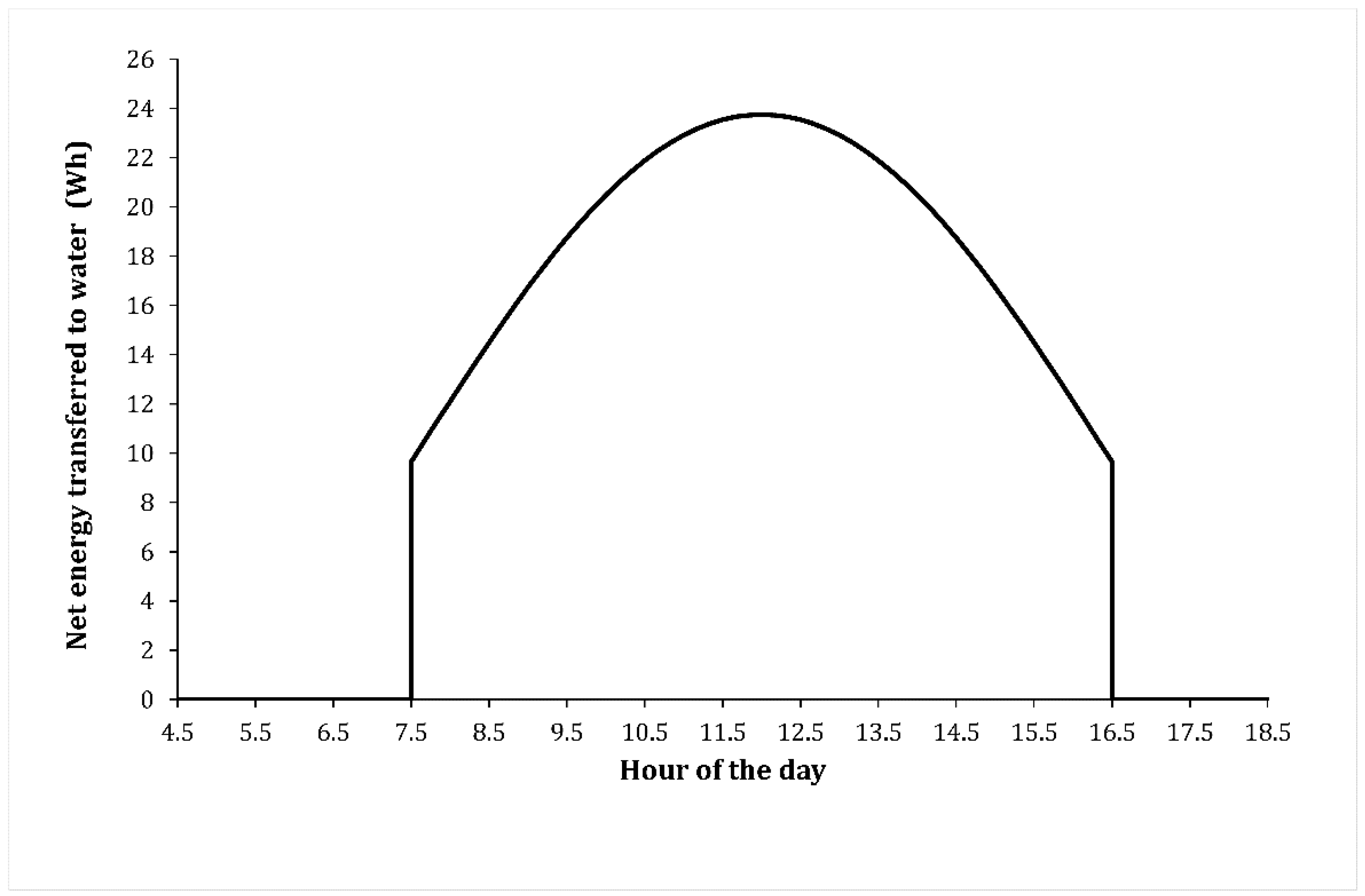
4.1. Irradiation Curves

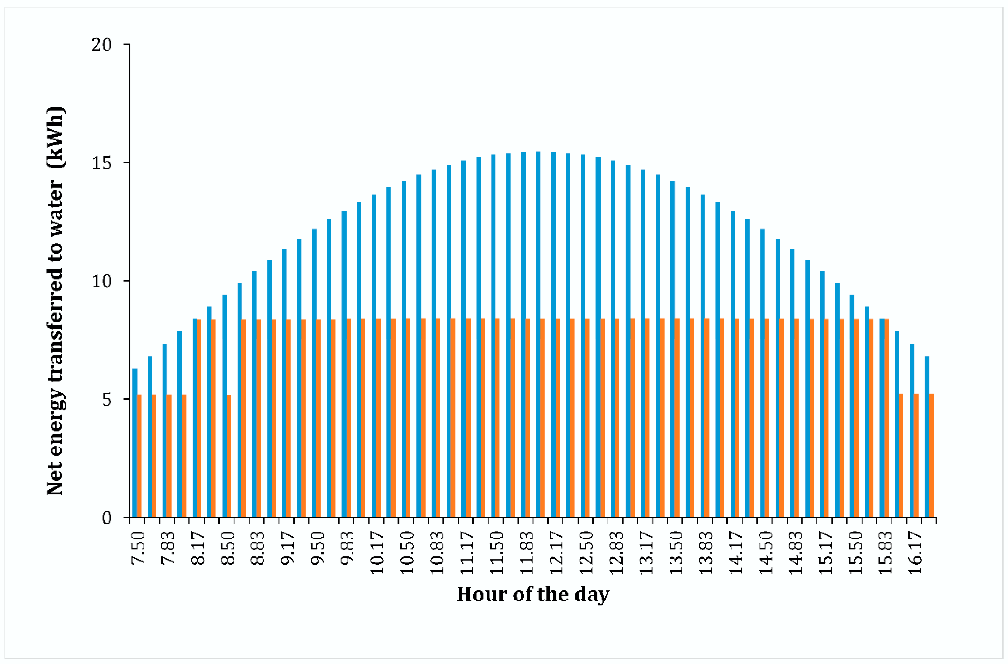
The monthly irradiation curves for the Albamix network are shown in Figure 1. These values were obtained with the formulas described in Appendix A. As 9 h is considered to be the time profitable for converting solar energy into shaft work in pumps, the net energy transferred to the water considers the nine hours of higher irradiance for a single PV panel (from 7.5 to 16.5 h; Figure 4).

4.2. Energy Requirements for Every Segment Combination

Water and energy audits were calculated using UAEnergy for every possible combination for the case study as shown in

Table 3. Shaft work required and minimum pressure at every node for every water requirement combination.

Combination	1	2	3	4	5	1-2	1-3	1-4
Injected flow (L/s)	85.1	84.4	85.4	85.3	84	169.5	170.5	170.4
Shaft work (Kwh)	5.24	5.20	5.26	5.25	5.18	8.41	8.42	8.42
Min Pressure (m.w.c.)	42.75	40.77	39.02	38.61	38.48	30.33	29.29	28.91
Combination	1-5	2-3	2-4	2-5	3-4	3-5	4-5
Injected flow (L/s)	169.1	169.8	169.7	168.4	170.7	169.4	169.3
Shaft work (Kwh)	8.40	8.41	8.41	8.39	8.43	8.41	8.40
Min Pressure (m.w.c.)	28.75	29.02	28.65	28.46	28.44	28.24	28.27

. As there were five sectors, the possible combinations of simultaneous water demands was ${{\displaystyle \sum }}_{i=1}^{n=5}\left(\begin{array}{c}n\\ i\end{array}\right)$ = 31. Combinations for 3, 4 and 5 segments opened simultaneously were not considered, as minimum pressure at some periods of the day was below the threshold pressure (combinations rejected for the current study). In short, there are only 15 possible combinations (five individual and ten combinations of two regions) for segments delivering water to crops.

4.3. Combinations Performed

The combinations should include a 5 × 54 matrix (5 rows, one per sector and 54 columns, one per every time step of 10 min, which produces an irrigation time of 9 h). The number of potential combinations is 5 × 2⁵³ (a very high value even for automated calculations). Some restrictions reduce this number of combinations, that is:

$$\begin{array}{c}{a}_{ij}=\{\begin{array}{ll} 1& if open\\ 0& if closed\end{array}\\ {\sum }_{j=1}^{j=54}{a}_{ij}=20\\ {\displaystyle {\displaystyle \sum }_{i=1}^{i=5}}{a}_{ij}\le 2\end{array}$$

(8)

The irrigation time should be higher than 194.9 min for July (Table 2) and, because every time step is 10 min, the irrigation time should be 200 min (20 periods with the subunit opened). As the minimum irrigation time is 1 h (six time step periods), irrigation of every sector should contain at least six consecutive values equal to 1. The following condition ${{\displaystyle \sum }}_{i=1}^{i=5}{a}_{ij}\le 2$ comes about as a result of it being impossible to irrigate more than two segments simultaneously (Table 3).

4.4. Results for the DPM Combinations

Finally, 10⁵ potential combinations meeting the restrictions above were created. For each combination, the $ceil\left[{\left(\frac{E_{req-i}}{E_{av-i}}\right)}_m\right]$ for the 54 time steps was calculated in order to know the number of solar panels required at every instant of the day to satisfy the i water demand. Of course, the maximum of these values results in the number of PVs necessary to satisfy water demand in these combinations. So, the number of solar panels for each of the 10⁵ potential combinations (a row vector of size (1, 1 × 10⁵) containing the panels required) was calculated. Among these, 60 combinations reached the minimum value of 651 solar panels (which returns the number of the modulus ($N_{mod}^{\ast }$) obtained at the m* combination.

To select the most appropriate value, the total energy required for these 60 combinations was calculated, and the selected combination should be the one with lower energy required, $m^{\ast }=\min \left({{\displaystyle \sum }}_i{E}_{req-i}\right)$ = 428.74 kWh. The selected DPM values are depicted in

Table 4. Demand pattern multipliers and energy consumption per time step.

Time	1	2	3	4	5	Time	1	2	3	4	5
0	1	0	0	0	0	4.50	1	0	0	1	0
0.17	1	0	0	0	0	4.67	1	0	1	0	0
0.33	1	0	0	0	0	4.83	1	0	1	0	0
0.50	1	0	0	0	0	5.00	1	0	1	0	0
0.67	1	0	0	0	1	5.17	1	0	1	0	0
0.83	1	0	0	0	1	5.33	1	0	1	0	0
1.00	0	0	0	0	1	5.50	0	1	1	0	0
1.17	1	0	0	0	1	5.67	0	1	1	0	0
1.33	1	0	0	0	1	5.83	0	1	1	0	0
1.50	1	0	0	0	1	6.00	0	1	1	0	0
1.67	1	0	0	0	1	6.17	0	1	1	0	0
1.83	1	0	0	0	1	6.33	0	1	1	0	0
2.00	1	0	0	0	1	6.50	0	1	1	0	0
2.17	1	0	0	0	1	6.67	0	1	0	1	0
2.33	0	1	0	0	1	6.83	0	1	0	1	0
2.50	0	1	0	0	1	7.00	0	1	0	1	0
2.67	0	1	0	0	1	7.17	0	1	0	1	0
2.83	0	1	0	0	1	7.33	0	1	0	1	0
3.00	0	1	1	0	0	7.50	0	0	0	1	1
3.17	0	1	1	0	0	7.67	0	0	0	1	1
3.33	0	1	1	0	0	7.83	0	0	0	1	1
3.50	0	1	1	0	0	8.00	0	0	0	1	1
3.67	0	0	1	1	0	8.17	0	0	0	1	1
3.83	0	0	1	1	0	8.33	0	0	0	1	1
4.00	0	0	1	1	0	8.50	0	0	0	1	0
4.17	0	0	1	1	0	8.67	0	0	0	1	0
4.33	1	0	0	1	0	8.83	0	0	0	1	0

, and the relationship between the energy consumed for these results and the energy available (as a result of the panels installed) is shown in Figure 5.

4.5. Comparison between Scenarios

Both Case 0 and Case 1 have the same injected volume of 5090.44 m³ (which takes into account that natural energy remains constant as the water level in the reservoir). On the one hand, the pumping system is more energy-hungry in Case 0 than in the case of operations with solar panels, Case 1. This is due to the fact that the irrigation time is much longer 16.8 (Case 0) vs 9 h (Case 1). On the other hand, this shorter irrigation time involves greater flow rates and accordingly, higher friction losses. Finally, useful energy is lower in Case 1 than in Case 0 (maintaining the pressure above standards at every node and every hour of the day;

Table 5. Results of the energy audit for Case 0 (irrigation time 16.8 h) and Case 1 (irrigation time 9 h).

	Case 0	Case 1
$E_N$ (kWh)	3134.95	3134.98
$E_B$ (kWh)	522.66	428.74
$E_U$ (kWh)	3634.87	3492.72
$E_F$ (kWh)	22.70	70.94

). This decrease shows better network operating efficiency as overpressure is avoided (with the benefits inherent to reduced pressure) while reducing the energy consumption in pumps (522.66 − 428.74 = 93.92 kWh/day).

5. Conclusions

This paper calculates the most efficient combination of hydrants and subunits to be opened simultaneously in an irrigation network, which minimize the number of solar photovoltaic panels and the energy consumption required to drive pumping devices directly connected to solar panels. This multi-objective optimization problem focuses on the consideration that water in irrigation networks should be delivered at pressures above the minimum threshold service pressure.

This approach should be undertaken after calculating crop water needs (when designing or when operating the network) and after network segmentation (creating a constant value for the injected flow). In order to reduce the environmental impact of the network operation, a solar energy source has been selected as a green alternative. This results in energy availability for a limited period of time (a consequence of the hourly irradiance curve) and an energy optimization problem arises. The solution to this new restriction involves making energy consumption as similar as possible to energy production. The energy consumption (shaft work in pumps) is a result of the irrigation network hydraulic behavior (with some other factors involved as friction, etc.) and this is calculated with the use of hydraulic simulation software. As this process is very time-consuming, programming software such as Matlab^® code has also been written to assist practitioners when dimensioning the PV array sets and another GUI (UAenergy) was also used for the energy audit calculations in networks.

The disadvantage of this approach is that if the irrigation schedule is created in a completely random way, the results obtained do not meet the restrictions (the most restrictive was to simultaneously supply no more than two segments for the whole simulation period; only 1 out of 10⁶ potential candidates). This meant that an ad-hoc algorithm needed to be performed to create the 10⁵ candidates (satisfying the requirements). It is noted that only 60 out of the 10⁵ candidates involved 651 solar panels and the candidate with the lowest energy consumption was 428.74 kWh per day.

Future research should focus on solving this problem for every month of the year and also trying to solve the problem considering every subunit as a single segment itself. In other words, analyzing the effect of being allowed to manage every water demand individually (e.g., in this case study, 132 segments should be analyzed).