Inferring the Economic Attributes of Urban Rail Transit Passengers Based on Individual Mobility Using Multisource Data

Abstract

Socioeconomic attributes are essential characteristics of people, and many studies on economic attribute inference focus on data that contain user profile information. For data without user profiles, like smart card data, there is no validated method for inferring individual economic attributes. This study aims to bridge this gap by formulating a mobility to attribute framework to infer passengers’ economic attributes based on the relationship between individual mobility and personal attributes. This framework integrates shop consumer prices, house prices, and smart card data using three steps: individual mobility extraction, location feature identification, and economic attribute inference. Each passenger’s individual mobility is extracted by smart card data. Economic features of stations are described using house price and shop consumer price data. Then, each passenger’s comprehensive consumption indicator set is formulated by integrating these data. Finally, individual economic levels are classified. From the case study of Beijing, commuting distance and trip frequency using the metro have a negative correlation with passengers’ income and the results confirm that metro passengers are mainly in the low- and middle-income groups. This study improves on passenger information extracted from data without user profile information and provides a method to integrate multisource big data mining for more information.

1. Introduction

With the development of information and smart city technology, urban big data, such as smart card data (SCD), call detail records (CDRs), and data from social media, such as Twitter, has become a new source for analysis of transportation demand and travel patterns [1]. These data are timely, offer wide coverage and relatively lower cost than traditional survey data [2,3]. However, these passively collected big urban datasets with heterogeneous structures lack some information, particularly individual attributes. Passengers’ socioeconomic attributes are important essential data for transportation demand analysis and forecasting [4]. Therefore, the investigation of individual attributes using urban big data is an important endeavor that can enrich data and offer the potential more in-depth study.

Urban big data mainly contain spatial and temporal information. This is especially true of SCD, which are normally nonregistered, contain no personal information at the raw data level, and exhibit home and work as the main activity locations with high regularity [5]. Therefore, much work so far has focused on identification of individual home and work locations using these data [6,7,8,9], while the inference of economic attributes has received less attention. Meanwhile, data from social media, which are registered, have been analyzed using several methods to infer individual attributes, including economic attributes, based on personal profiles in raw data. However, these data are difficult to integrate into transportation analysis. As a result, research on travel pattern analysis with socioeconomic attributes is generally conducted based on survey data [10,11]. However, the timeliness of survey data may affect the validity of results, which does not promote understanding of travel pattern changes of the travelers under the condition of fast-growing urban transportation and makes it difficult to guide the improvement of transportation policies. Consequently, the inference of travelers’ economic attributes from urban big data without personal profiles has significant importance for transportation analysis.

Previous research has verified that travelers’ economic attributes are related to individual mobility [10,11]. More specifically, people with specific trip purposes will focus on locations that can satisfy these goals and subsequently complete their trips at locations suitable to their economic status [12]. Therefore, the relationship between individual mobility and economic attributes provides a novel way to infer an individual’s economic status using big data, especially for data such as SCD that does not contain personal profile information [12]. However, any study on economic attribute inference for smart card users has, to date, not been attempted. Therefore, this study formulates a method to detail the economic attributes of smart card users based on the relationship between individual economic attributes and passenger mobility [13]. In addition, this method serves as a common analytical framework for inferring individual economic attributes using data without personal profiles.

The remainder of this paper is organized as follows. Section 2 reviews and analyzes related works. Section 3 proposes a model framework to infer travelers’ economic attributes by integrating SCD with other urban data. The model framework is applied to data from Beijing and the results are reported in Section 4. Section 5 discusses the results and the method. Finally, Section 6 contains the conclusion.

2. Literature Review

The lack of individual attributes is a general disadvantage of urban big data. Therefore, the inference of individual attributes has been actively studied in urban data research. Most studies focus on data with user profiles such as social media data, which are produced by registered entities.

For advertising purposes, user profile data and tweets have generally been used to mine latent user attributes [14]. Daniel et al. [15] mapped Twitter users’ job titles with an annual survey of hours and earnings for various job classes to discover individuals’ mean yearly income and analyzed the interplay between user emotions and sentiment and income. In addition, the tweet content and behavior of Twitter users are strongly related to their socioeconomic status [16]. Based on this relationship, machine learning algorithms [17] and deep learning methods [18] are used to predict certain personal attributes, and the results can achieve satisfactory precision. Meanwhile, Aletras and Chamberlain [19] conducted an in-depth analysis of the relationship between income and social network structure and written content and used the model to predict user income. Multisource data can provide more perspectives than a single data source from which to derive solutions. Examining the CDRs of the caller and the person called can establish a stronger and truer relationship network. Meanwhile, the phone number can be used to combine this social network with banking information [20]. Consequently, a Bayesian approach could be used to infer other users’ economic status based on known users’ communication network characteristics [20,21]. Location features can also be integrated with social media check-in data to infer users’ demographic attributes, and the results have been verified by registered user profiles [12].

Data without user profiles produced by nonregistered entities, such as SCD, has received less attention in terms of the inference of individual economic attributes. However, many studies have demonstrated that economic attributes are related to individual trip patterns. Populations with higher socioeconomic levels are strongly linked to larger mobility ranges than populations with lower income levels [22], with diversity of mobility exhibiting a strong correlation with socioeconomic attributes [23]. Besides, trip chain type choices and non-work stops in a trip chain are strongly distinct between income groups [24]. Meanwhile, trip pattern analysis based on SCD has shown that the activity sequence structure category is associated with income for full-time employment [25]. In addition, traditional trip survey data has shown that passengers’ income is correlated with their commuting distance [11,26]. Because the urbanization rate significantly impacts the commuting time for different income levels [27], different relationships have been found in studies of different countries [11]. Therefore, this relationship provides a method to infer individual economic attributes using data without user profiles.

From the above, most previous studies have overlooked the relationship between individual mobility and economic attributes, which can be used to infer individual economic status. In practice, individuals’ economic and consumption attributes are related to the economic characteristics of the places they visit, such as living or entertainment costs, and to mobility features such as visit frequency, mobility diversity, and commuting distance. Integrating location features with passengers’ mobility characteristics could be a novel solution to the inference of individual economic attributes.

Based on the relationship between individual economic attributes and passenger mobility [13], this study built a mobility to attribute (M2A) framework to detail the economic attributes of smart card users. It was developed based on three kinds of urban data: SCD, shop consumer data, and house price data [28]. SCD, which record visited stations of each passenger, can be used to generate individual mobility. Shop consumer data and house price data, which are collected from the Internet, can identify location economic features. The framework integrates these data to formulate passengers’ consumption attributes. Based on the consumption attributes, their economic levels can be inferred. We used this framework to systematically infer individual economic attributes and analyze individual mobility using urban data of Beijing.

3. Methods

The inference framework, M2A, is shown in Figure 1. It includes two steps: individual mobility formulation and economic attributes inference. In order to formulate individual mobility, trip chains should be generated from SCD. Then individual mobility is described using commuting distance, mobility diversity, home location, and other types of activity locations extracted from the trip chains. Next, from individual mobility to individual attribute, location economic profile should be calculated using house price and shop consumer price. Then, passengers’ economic attributes are described by their mobility indicators and visited stations, mapped with the location economic profiles, including inferior good consumption, normal good consumption, and superior good consumption. Finally, a comprehensive consumption attribute is formulated for each passenger and his/her consumption levels are classified using a clustering method.

3.1. Mobility Formulation Model

3.1.1. Extraction of Trip Chains

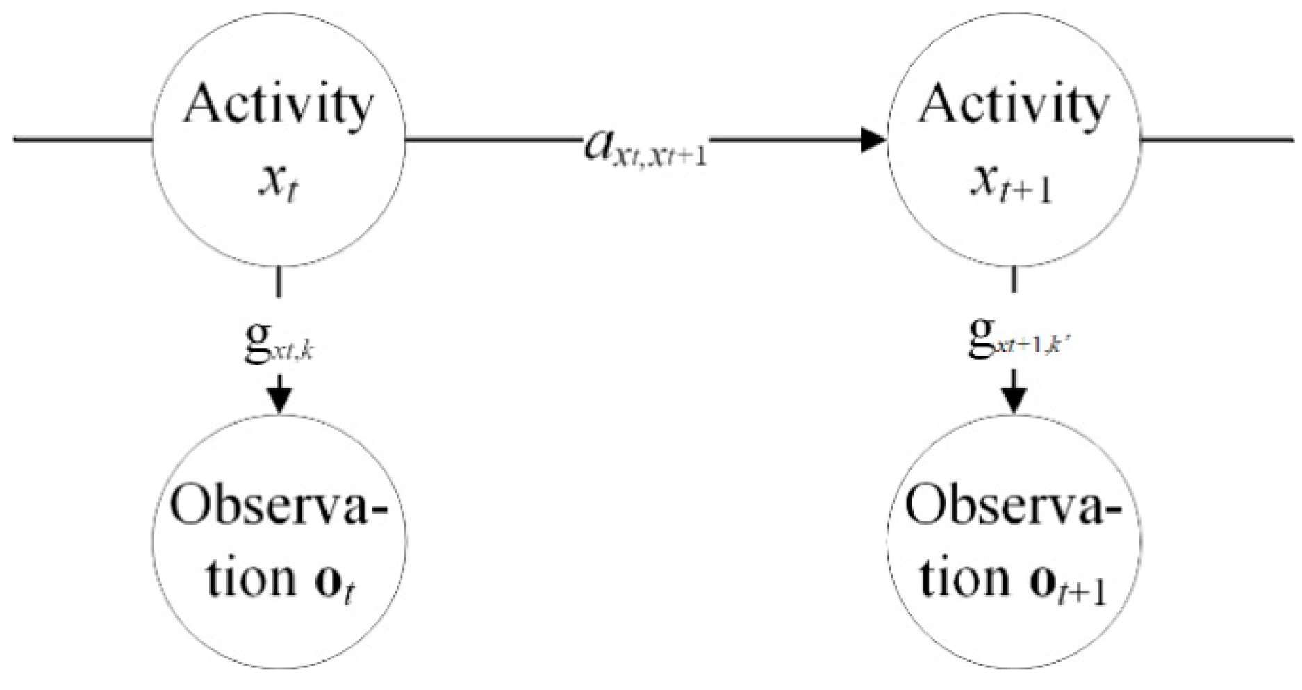
Trip chains are base data for analyzing passengers’ mobility. Some studies have verified that trip chains inferred from urban big data are different from traditional survey data and more reasonable than traditional survey data [29,30]. For SCD, a trip chain of each card number without trip purpose can be formulated in a chronological order by trip time. Therefore, the major task is to infer trip purpose for each trip in all trip chains. Most existing methods that model individual mobility are based on the Markov Chain (MC) [31] and, hence, this study formulated a hidden Markov model (HMM) to infer trip purpose, as illustrated in Figure 2.

In a trip chain, trip purpose, or activity type [32] x_t is a hidden state in hidden state space HS with J states. A hidden state may perform as observation state k in observation state space OS with K states and its emission possibility of g_xtk. For hidden states, the following state can only be affected by the current state, so the transition probability between hidden states is a_xtxt+1.

Trip purpose or activity type mainly relates to three elements: activity start time, land usage of destination, and stay duration, especially for commuting trips [6,7,8,9]. Therefore, an activity with all three elements is chosen to analyze trip purpose. More specifically, an activity is identified when the exit station of a trip is the same as the entry station of the next trip, according to the records of one card number. Activity start time can be defined as the exit time, while staying duration can be described as the exit time of the trip subtracted from the entry time of the next trip.

Mapping to the HMM, the observations are the three elements of activity and, hence, the observable parameter set o^l_t of the tth activity in the lth trip chain can be constructed as Equation (1), in which s^l_t is the activity start time, d^l_t is the stay duration, and c^l_t is the vector of the degree of land usage mixture of the station that can be inferred from passenger flow distribution at the station [33,34]; for more detailed information, see Yue et al. [35].

$${\mathbf{o}}_t^l=\left(s_t^l,d_t^l,{\mathbf{c}}_t^l\right)$$

(1)

In this model, observations are continuous variables and, thus, they should be classified into a discrete observation state space OS with K states. Assuming that observations of state k in every trip chain are Gaussian distributions with µ_k as the mean value and σ_k as the variance, observation o_t is classified under state k using Equation (2):

$$k=\underset{k\in OS}{\arg \max }f\left({\mathbf{o}}_t|{\mathsf{\mu }}_k,{\mathsf{\sigma }}_k\right)$$

(2)

Then, a discrete time-homogeneous Markov model is formulated [36]. Comparing with standard HMM, a discrete processing using Equation (2) is added into it. In addition, the optimal parameter set is λ = [π, A, G, µ, σ], in which the initial activity is π = (π₁, π₂, …, π_M), the transition probability is A = (a₁₁, a₁₂, …, a_J,J−1, a_J,J), the emission possibility is G = (g₁₁, g₁₂, …, g_J,K−1, g_J,K), the observations’ mean value is µ = (µ₁, µ₂, …, µ_K−1, µ_K), the variance is σ = (σ₁, σ₂, …, σ_K−1, σ_K), and the total number of trip chains is M. According to the observed trip chains, the optimal parameter set can be estimated using the Baum–Welch and forward–backward algorithms [9,36].

To infer trip purpose, the Viterbi algorithm [36] was improved and adapted in this model, as indicated, in Equation (3). V_t,xt is the probability value of hidden state x_t corresponding to observation o at t based on the former states. After all trips in a trip chain are calculated, the state chain with the largest probability is the trip purpose of the corresponding trip chain and the trip chains with their trip purposes are extracted from SCD.

$$V_{t,x_t}=\underset{j\in HS}{\max }\left(V_{t-1,j}{a}_{j{x}_t}\right)\underset{k\in OS}{•\max }\left(g_{x_{t}k}{f}_{\mathbf{o}k}\right)$$

(3)

3.1.2. Individual Mobility

Commuting distance and mobility diversity have a correlation with each passenger’s economic attributes [11,23,26]. Commuting distance is calculated as the shortest path in the network between the station where home is located and the station where work is located for the passenger. All other types of activities, including shopping, entertainment, and eating, can be used to describe mobility diversity that is measured using the Shannon entropy [13,23].

In this study, three trip purposes are identified: going home (H), going to work (W), and other-type (O). Consequently, home location (S_H) and work (S_W) location are identified to calculate commuting distance using rule-based method, as shown in Figure 3.

As for home and work location, they generally are fixed for each passenger [7,37]. Therefore, destination stations and frequency of trip purpose H and W are computed for every passenger. Then, the locations are identified as the stations with the highest corresponding frequency. However, if there are multiple stations with the highest frequency for trip purpose H/W, the corresponding location is identified as the station with the highest proportion of residential/office land usage. Finally, each passenger’s commuting distance (cd) is calculated using the Dijkstra algorithm.

Meanwhile, destination stations with trip purpose O {S₁, …, S_M} are also extracted to measure mobility diversity. The mobility entropy E(u) of individual u is shown in Equation (4). D is the set of all trip destination stations, p(d) is the probability of station d, and H is the total number of trips.

$$E\left(u\right)={\displaystyle \sum _{d\in D}p\left(d\right)\log p\left(d\right)}/\log H$$

(4)

Finally, for each passenger u, we can formulate his/her individual mobility characteristic IM^u by Equation (5).

$$I{M}^u=\left(c{d}^u,H^u,S_H^u,\left\{S_1^u,\dots ,S_{M^u}^u\right\},E\left(u\right)\right)$$

(5)

3.2. Attributes Inference Model

Individual mobility characteristics are related to economic attributes. The visited locations contain far more information than just the category [12], and the location’s economic feature is related to its visitors’ economic attributes. More specifically, the price of their family home can reflect their affordable living cost, and the price of goods in their visited shops can reflect their consumption level. Consequently, location’s economic features can be used to further detail passengers’ economic attributes. In this study, a location’s economic feature is derived from two aspects: living cost and entertainment cost.

3.2.1. Location Economic Feature

Living cost is captured by the rental or sale price of a house in the range of a station’s catchment area, as shown in Equation (6). In the equation, av_s is the average sale price, av_r is the average rental price, v_s is the variance value of the sale price, and v_r is the variance value of the rental price.

$$\mathbf{LC}=\left(a{v}_s,a{v}_r,v_s,v_r\right)$$

(6)

The entertainment cost at a station can be formulated by the average price and variance of each shop type in its catchment area, as indicated by Equation (7). In the equation, av_c is the average price value of shop type c, v_c is the price variance of shop type c, and N_c is the total number of shop types c, c = (1, 2, 3).

$$\mathbf{EC}=\left(a{v}_1,a{v}_2,a{v}_3,v_1,v_2,v_3,N_1,N_2,N_3\right)$$

(7)

3.2.2. Individual Consumption Characteristic

From the above, each passenger’s consumption characteristic can be formulated by integrating his/her individual mobility characteristic and location feature. For analyzing the relationship between consumption behavior and individual economic attributes (income level), income elasticity of demand (IED) is introduced from economics. IED is defined as the ratio of the percentage change in the demand for a good to the percentage change in consumer income measured by the income expenditure (price) for the good [38,39,40] to describe the economic feature of the good. In accordance with value of IED, three types of goods can be classified as inferior goods (IED < 0), such as bus travel and canned food, normal goods (0 < IED < 1) such as a house and food, and superior goods (IED >> 1) such as entertainment and fashion items [40].

This study derived smart card user’s consumption characteristic from three aspects, inferior good consumption, normal good consumption, and superior good consumption.

• Inferior good consumption (IGC)

The most common view of public transit is as an inferior good, which means as income rises, people will travel less by public transit; however, this is often debated [41,42]. Holmgren [41] reviewed 22 IED values for public transit, and found a range of −0.82 to 1.18, with a mean of 0.17. This shows that the usage of public transit is highly dependent on a passenger’s income, but the relationship is ambiguous.

Here, we assume that public transit is an inferior good and the expected IED is negative. Indicators of commuting distance and total number of trips using the subway for each passenger are chosen to describe inferior good consumption. Then, the relationship between these indicators and individual economic attributes are analyzed to test this assumption.

• Normal good consumption (NGC)

Housing has been verified as a normal good, and the IED value ranges from 0.69 to 1.43 [38,39,43]. More specifically, IED values in China range from 0.786 to 1.430 with an average of 1.044 [43], which indicates that as income rises, people increase housing expenditure, and the increment is approximately equal to the income increment.

In this study, the living cost of each passenger’s home location is chosen to measure the normal good consumption. In addition, we assume that the expenditure distribution on normal goods for all passengers is consistent with their income distribution, and the relationships between other factors and income are consistent with the relationships between them and passengers’ living costs.

• Superior good consumption (SGC)

A superior good is generally viewed as a special normal good that has a higher IED value. Dining out, shopping, and entertainment have been verified as superior goods in some research [44,45] and are always related to activities other than working and staying at home.

Therefore, the mobility of the other-type activity and the corresponding location’s economic features are used to formulate each passenger’s superior good consumption. More specifically, for each passenger, entertainment expenditure is calculated using the station entertainment costs of all stations visited for other-type activities by Equation (8) [46]. The passenger’s superior good consumption is described using entertainment expenditure and mobility diversity.

$$\begin{array}{c}a{v}_c^u=\left(a{v}_{c1}+a{v}_{c2}+\dots +a{v}_{c{M}^u}\right)/M^u\\ v_c^u=\left[v_{c1}\left(N_{c1}-1\right)+v_{c2}\left(N_{c2}-1\right)+\dots +v_{c{M}^u}\left(N_{c{M}^u}-1\right)\right]/\left(N_{c1}+N_{c2}+\dots +N_{c{M}^u}-M^u\right)\end{array}$$

(8)

where av_c^u is average expenditure in shop type c of passenger u, M^u is the total number of stations visited for other-type activities of passenger u, av_cm is average cost of shop type c of station m, v_c^u is pooled expenditure variance in shop type c of passenger u, v_cm is cost variance of shop type c of station m, N_cm is the total number of shop type c of station m, and c = (1, 2, 3), m = (1, 2, …, M^u).

3.2.3. Economic Attributes Inference

Based on these consumption indicators, a comprehensive consumption indicator set C^u is formulated for passenger u, as shown in Equation (9), and all terms are as previously defined.

$${\mathbf{C}}^u=\left(\underset{\mathrm{IGC}}{\underbrace{c{d}^u,H^u}},\underset{\mathrm{NGC}}{\underbrace{a{v}_s^u,a{v}_r^u,v_s^u,v_r^u}},\underset{\mathrm{SGC}}{\underbrace{a{v}_1^u,a{v}_2^u,a{v}_3^u,v_1^u,v_2^u,v_3^u,E\left(u\right)}}\right)$$

(9)

To reduce the correlation among variables, the principal component analysis (PCA) is used to extract the principal components of the indicators. Then, a k-means clustering method is used to obtain passengers’ consumption levels, and the optimal number of clusters is chosen by the Davies–Bouldin criterion [47]. These levels are passenger economic attribute levels.

4. Model Implementation and Results

This study utilizes one-week SCD from the Beijing subway for March 2016, consumer data for the shops around the subway stations for 2016, and house sale and rental price data for 2016 to implement the M2A framework.

4.1. Data Preparation

Urban big data are collected passively and include abundant bad and redundant data. Therefore, they need to be cleaned and preprocessed initially. To simplify, we assume passengers come from or are destined for a location within walking range of a station, and do not require other transportation modes.

From SCD, card ID, entry line and station ID, entry time, exit line and station ID, and exit time are extracted from a large number of fields. Then, line and station ID are replaced by station name to identify passengers going to an interchanging station from different entrances from one station. Finally, the data are cleaned by deleting the records in which the entry and exit stations are identical or the exit time is earlier than the entry time. After preprocessing and data integrating, 50,141 passengers’ trip records remain to be analyzed.

Shop consumer data are collected from a business review website, dianping.com, in China that is similar to Yelp in the US. The data contain five items: station name, every shop name, every shop location, average price of each shop, and review score of each shop. First, we calculate the Euclidean distance between shops and the nearest stations and filter the shops by a distance of more than 800 m. Then, according to shop categories (c), which are catering, entertainment, and shopping, we calculate the average price (av) and price variance (v) of consumption for every station using Equations (10) and (11):

$$a{v}_c={\displaystyle \sum _{i=1}^{N_c}p{r}_i•c{f}_i}/N_c$$

(10)

$$v_c={\displaystyle \sum _{i=1}^{N_c}{\left(p{r}_i•c{f}_i-a{v}_c\right)}^2}/N_c$$

(11)

where N_c is the number of shops in category c in the catchment area of a station, pr_i is the average price of the ith shop, and cf_i is the ratio of the review score of the ith shop to the sum score of all category c shops, which reflects the attractiveness of a shop.

Shop consumer data of Xizhimen station, available online, are used to show the preprocessing. First, we group the shops into three categories based on their types; then, we calculate the average price and price variance for each category. Considering the example of catering-type shops, there are three items to review on a 10-point scale for each shop; these items describe taste, environment, and service. For each item, we calculate the average score and assign it to the missing shops. We sum all of the scores to obtain the total score ts_i for each shop and the average total score for the catering-type shops in the Xizhimen area, as = 22.29. The attractiveness of each shop is calculated as cf_i = ts_i/as. Integrated with the price of each shop, the average price of catering in the Xizhimen area is formulated using Equation (1), av_cater = 45.92. Based on the average price, the price variance can be calculated using Equation (2), v_cater = 1261.67. The same processing is used for entertainment and shopping in the Xizhimen area, the average price and price variance can be calculated as, av_enter = 36.02, v_enter = 999.82, av_shop = 477.5, v_shop = 415,973.4.

The house price data are collected from a real estate website. They contain three items: station name, house location, and rental or selling price. Houses that are located in the catchment area of 800 m are chosen for the analysis.

4.2. Model Implementation

First, we implement HMM based on the algorithm flow, as shown in Figure 4; a separate numerical simulation study was conducted [48]. From the results, we identified six observation clusters, as shown in

Table 1. Clusters of observation states.

	Cluster 1	Cluster 2	Cluster 3	Cluster 4	Cluster 5	Cluster 6
Activity start time	9:22	8:16	9:50	15:47	16:34	19:13
Duration/min	468.54	613.33	149.56	136.20	1022.62	763.40

. Based on the observation clusters, four activity types were inferred with three trip purposes, as presented in

Table 2. Results of trip purpose inference.

	Cluster 1	Cluster 2	Cluster 3	Cluster 4	Cluster 5	Cluster 6	Trip Purpose
Activity 1	0.221	0.751	0	0	0	0.028	Work
Activity 2	0.236	0.015	0.24	0.221	0.2	0.088	Other
Activity 3	0	0	0.001	0.016	0.074	0.908	Go home
Activity 4	0.763	0.115	0.044	0.078	0	0	Work

. Activities 1 and 4 are included in the trip purpose of “Work”, which may be because of different attendance management of different companies in Beijing.

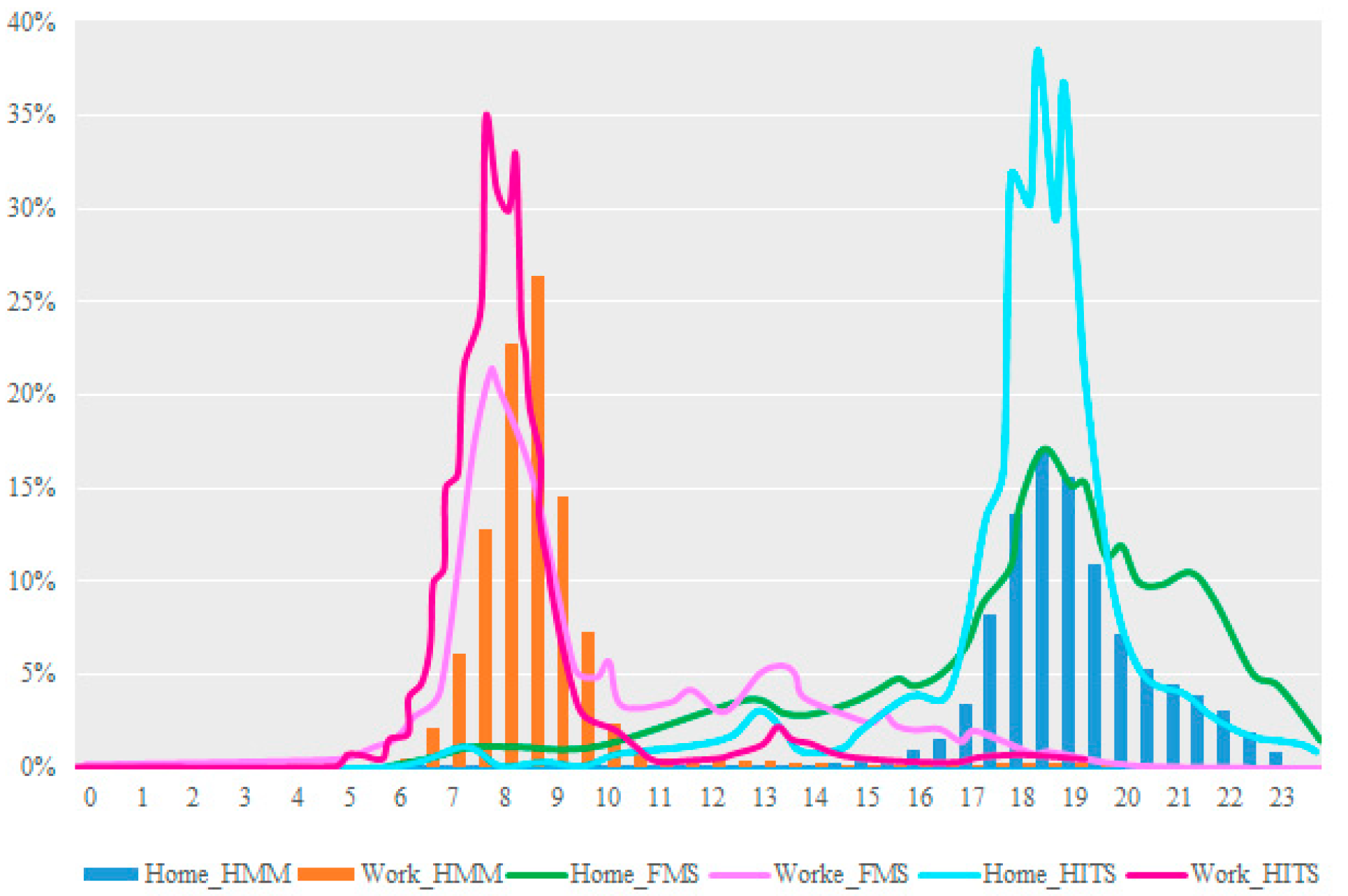
Based on these results, each passenger’s trip purpose is inferred from the SCD to generate trip chains using HMM; the percentages of passengers traveling to work and home at different times of the day are shown in Figure 5. Due to a lack of detailed survey data for Beijing, the results of the Household Interview Travel Survey (HITS) and the Future Mobility Survey (FMS) in Singapore [49] are used to verify the results of this study. Based on these, the results of this study using HMM are consistent with the results of the FMS during peak hours, while they match better with the results of HITS during off-peak hours. Because trip purposes during peak hours mainly are going home or to work [6,7], they have higher regularity and predictability than other periods [5]. In this study, HMM can capture these trips with high accuracy as does the FMS [49]. During off-peak hours, trip purposes vary; however, this study only analyzed continuous trips by metro using smart cards. Therefore, its limited sample size may lead to under-reporting of related trips as in the HITS [49]. Notably, in the results of the HITS and FMS, the morning peak is earlier than in the HMM result. This is because work time is earlier in Singapore than in Beijing. From the above, accuracy of the results of HMM is similar to or even higher than that of the HITS and are suitable for in-depth analysis.

Subsequently, individual mobility is derived from the trip chains. The location economic feature data are combined, the comprehensive consumption indicator set of each passenger is formulated, and five principal components are extracted, as show in

Table 3. Rotated component matrix of principal component analysis (PCA).

	1	2	3	4	5
cd	−0.607	−0.026	−0.044	−0.091	0.022
H	−0.03	−0.002	−0.007	−0.007	0.832
avs	0.84	0.015	0.026	0.204	−0.031
avr	0.905	0.02	0.045	0.08	−0.006
vs	0.808	0.011	0.013	−0.002	−0.02
vr	0.532	−0.017	−0.027	−0.154	0.046
av1	0.039	0.216	0.933	0	0
av2	0.021	0.974	0.164	0.002	0.004
av3	0.082	−0.001	−0.006	0.929	0.001
v1	0.034	0.095	0.957	−0.003	−0.001
v2	0.019	0.977	0.147	0.004	0.004
v3	0.046	0.005	0.002	0.932	−0.006
E	0.015	0.009	0.006	0.001	0.834

. The first component includes the information of commuting distance and living cost. However, commuting distance shows negative relationship with living cost significantly. This result means as income rises, people will travel shorter to commute by public transit, and it confirms that public transit is an inferior good for the commuting trip. Catering, entertainment, and shopping consumption are three different components, respectively. It shows they have a different relationship with income. At last, trip frequency and mobility diversity are in the same component, which means they have the same relationship with income.

4.3. Results

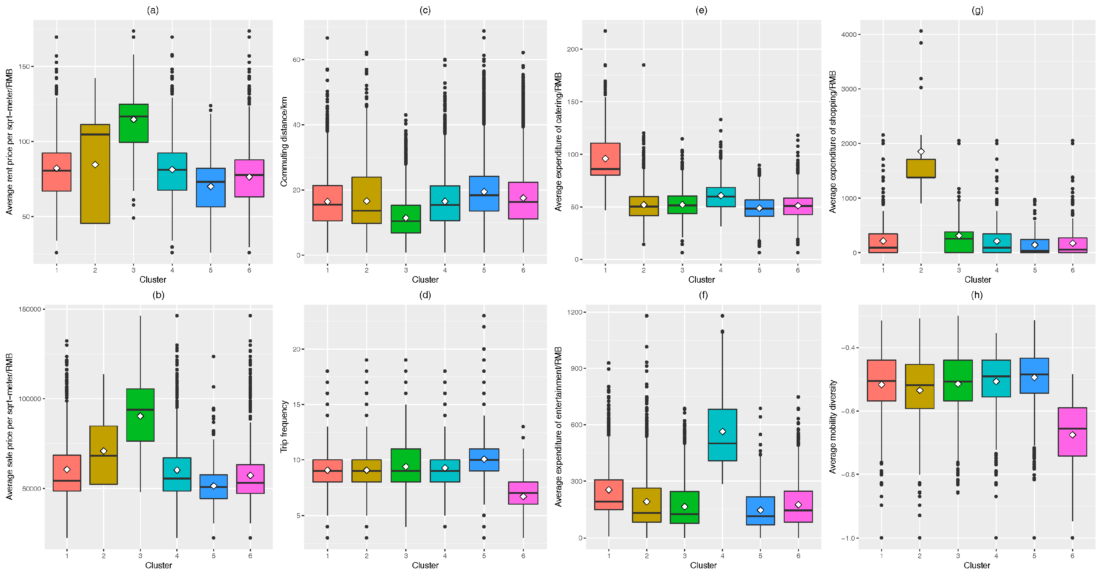
At last, six consumption levels are classified using k-means method, as shown in Figure 6.

From Figure 6a,b, we can claim that passengers in cluster 3 have the highest income among all the metro passengers, followed by cluster 2, based on our assumptions. Furthermore, clusters 1 and 4 are the middle-income groups and clusters 5 and 6 are the low-income groups. Considering the distribution of commuting distance in Figure 6c, it has a negative relationship with metro passenger income. As for superior consumption, clusters 3, 5, and 6 maintain a low expenditure on catering, entertainment, and shopping. High-income passengers have more options, such as private cars or taxis, for flexible trips like shopping, while low-income passengers are constrained by ratio of expenditure to income [50]. Therefore, they take fewer superior consumption trips via the metro than other passengers and their expenditure is lower than others. Interestingly, other passengers have different consumption preferences for superior goods. Passengers in cluster 2, who have higher income than those passengers of clusters 1 and 4, prefer to take the metro to high consumption areas of shopping, while passengers in cluster 1 prefer to take the metro to expensive eating areas and spend more money on dining outside, and passengers in cluster 4 prefer to travel to expensive entertainment by metro. Individual trip frequency and mobility diversity by metro have no significant correlation with passenger income, as evident from Figure 6d,h. More specifically, the average trip frequency is about nine for all clusters, excluding cluster 6; this implies that these passengers mainly use the metro for commuting.

5. Discussion

In-depth analysis on home locations of different income levels is shown in Figure 7. Homes of high-income passengers are mainly located in the north of the city center, as shown in clusters 2 and 3. Homes of low and middle-income passengers are mainly located outside the city center; and, some of them in clusters 5 and 6 are located in the north of the suburbs. This result is consistent with the observation from Mohamed et al. [10] which also shows high-income passengers mainly live in downtown areas and low-income passengers mainly live in suburban areas.

Note that home and work locations are fixed for each passenger, and that other-type activities can reflect passengers’ mobility diversity more adequately. Therefore, we analyzed the other-type activities for each cluster; their spatial distributions, shown in Figure 8 suggest significant relations with the economic groups. All of them show significant positive spatial autocorrelation (Moran’s I > 0, p = 0), but for high-income passengers in clusters 2 and 3, the activity locations have a stronger spatial autocorrelation than the other clusters because of larger Moran’s I values, implying that these locations have a higher spatial aggregation. Furthermore, the frequently visited stations are mainly located in the north of the city; this spatial character is similar to the spatial distribution of their homes. For middle-income groups (clusters 1 and 4), the frequently visited stations are mainly located in the Guomao (GM), Wangfujing (WFJ), and Chaoyangmen (CYM) regions. These regions have high consumption levels, especially of catering and entertainment, and therefore these passengers’ expenditure on catering and entertainment is high. Low-income groups have numerous frequently visited locations in the entire city region, including the south of the city, and they have a low spatial aggregation. Other-type trips of low and middle-income passengers show that the comprehensive development of land around public transit stations in suburban areas is lower than that around those stations in the city center. Therefore, passengers are obliged to take public transit from their suburban homes to the city center for catering, entertainment or shopping. Consequently, for government decision-makers, comprehensive development of land around suburban stations may afford greater convenience to low and middle-income citizens.

Next, a Pearson correlation coefficient is calculated between living consumption indicators and other consumption indicators for quantitative analysis, as shown in

Table 4. Pearson correlation coefficients between housing sale price and other indicators.

avs	Cluster 1	Cluster 2	Cluster 3	Cluster 4	Cluster 5	Cluster 6	All
cd	−0.360 **	−0.518 **	−0.160 **	−0.381 **	−0.272 **	−0.321 **	−0.415 **
H	−0.060 **	−0.099 **	−0.063 **	−0.044 **	0.041 **	−0.145 **	−0.038 **
av1	0.080 **	0.201 **	0.111 **	0.005	0.053 **	0.081 **	0.055 **
av2	0.045 **	0.135 **	0.109 **	0.155 **	0.021 **	0.046 **	0.033 **
av3	0.264 **	0.260 **	0.034 **	0.235 **	0.155 **	0.254 **	0.225 **
E	−0.008	−0.108 **	−0.081 **	−0.039 **	0.012	−0.128 **	−0.010 *
Sample (%)	8.45	5.07	18.41	11.99	37.55	18.53	100

Note: * and ** denote statistical significance at 95% and 99% confidence, respectively. Items of interest are marked by bold.

and

Table 5. Pearson correlation coefficients between housing rental price and other indicators.

avr	Cluster 1	Cluster 2	Cluster 3	Cluster 4	Cluster 5	Cluster 6	All
cd	−0.458 **	−0.614 **	−0.034 **	−0.457 **	−0.401 **	−0.410 **	−0.481 **
H	−0.037 *	−0.103 **	−0.084 **	−0.036 **	0.048 **	−0.127 **	−0.029 **
av1	0.093 **	0.243 **	0.108 **	0.039 **	0.074 **	0.090 **	0.082 **
av2	0.053 **	0.149 **	0.123 **	0.103 **	0.041 **	0.051 **	0.047 **
av3	0.212 **	0.203 **	−0.202 **	0.164 **	0.129 **	0.223 **	0.136 **
E	−0.009	−0.109 **	−0.088 **	−0.024	0.008	−0.107 **	−0.003

Note: * and ** denote statistical significance at 95% and 99% confidence, respectively. Items of interest are marked by bold.

. Overall, commuting distance and trip frequency have a significantly negative correlation with passengers’ living consumption expenditure that can be used to represent their income based on our assumption. This result verifies that public transit is an inferior good. Average expenditures for catering, entertainment, and shopping have significantly positive correlations with passengers’ living consumption expenditure, while mobility diversity has a negative relationship with living consumption but this relationship is not significant for housing rental expenditure. This reveals that passengers with high-income do not prefer to take the metro to a new place as they have alternative modes to choose from [50].

Based on group dimensions, as a high-income group, cluster 3 has a lower correlation between income and commuting distance, as marked by bold. This indicates that high-income passengers may have a longer trip to work; this relationship has been indicated in previous studies as well [11,26,27]. Further, the correlation with shopping expenditure is lower or even negative, which indicates that high-income passengers do not prefer to take the metro to shop. For cluster 2, which is the second highest income group, this group has a higher correlation with all types of superior consumption because they have more disposable income to afford such consumption. For the middle-income groups, there is only one type of superior consumption with a high correlation—for cluster 1 it is shopping—although they generally go to expensive eating areas and spend more money on eating away from home; and for cluster 4, it is entertainment. In addition, their mobility diversity shows no significant correlation with their income. From the data in the two tables, passengers in cluster 6 have higher income than those in cluster 5. Because cluster 5 has a positive correlation with trip frequency, this indicates that these passengers have a strong dependency on public transit. Meanwhile, passengers in cluster 6 have a higher correlation with shopping expenditure than most other groups. However, cluster 5 represents a large share of the studied passengers, indicating that 37.55% of the passengers are low-income and they have a strong dependency on the metro for their daily trips. This result is consistent with the survey result of Beijing that claims that metro passengers are mainly low and middle-income people [51]. From an overall perspective, shopping consumption is strongly related to passenger’s income, especially for low and middle-income passengers. In combination with the home location distribution of these passengers, this indicates that comprehensive shopping malls are needed for suburban stations. An improved land usage mix could reduce these other-type trips, and afford greater convenience. This would also embody the principles of transit-oriented development (TOD).

Based on our analysis and discussion, this model framework can perfectly infer passengers’ economic attributes from SCD without user profiles, and some results have been verified by previous studies. However, several limitations exist in this study. The first is result validation from an individual perspective. This study focuses on economic attributes inference using big data without user profiles, and the raw data lack individual information. Based on this limitation, we introduce the second, which is that the income amount cannot be calibrated, and we are able to obtain only the relative income level. Therefore, more detailed survey data should be considered for in-depth analysis in the future. Finally, as a preliminary work to infer travelers’ economic attributes using urban big data without user profile information, this study formulates the model framework using certain default assumptions such as activity location, which is considered as the walking-distance range from an exit station without transferring to other modes. This limitation can be avoided by taking more data sources into consideration.

6. Conclusions

Most studies mainly focus on the inference of individual economic attributes using big data with user profile information, like occupation and phone number, which can be used to integrate other economic data. Data without user profile information, like SCD, have not been considered for individual economic attributes inference. This study fills this gap by formulating a M2A framework based on the relationship between individual mobility and economic attributes.

The M2A framework integrates individual mobility characters with location features to infer passenger economic attributes. Using this framework, a case study of Beijing is implemented. From the results, we confirm that commuting distance and trip frequency using the metro have a negative correlation with passengers’ income. However, some high-income passengers may have a longer trip distance to work, which has also been found in previous studies. High-income passengers mainly live in the city center, while low and middle-income passengers mainly live in suburban areas. However, low and middle-income passengers prefer to shop in the city center, because suburban stations generally lack comprehensive land development. Therefore, improving the land usage mixture around suburban station is needed for TOD. In addition, for the middle-income group and the second highest income passengers, they can afford more types and more expensive superior goods. As for low-income passengers, who make up a larger part of the metro ridership, they have a strong dependency on the metro for their daily trip.

Based on the limitations of this study, acquiring more data sources such as SCD of the bus system, bike sharing system data, or even CDRs would be suggested for future work. These data can provide more detail on travelers’ activity characteristics for inferring more accurate economic attributes. Further, long-period data also can effectively improve the results, which can reflect individual travel preference for various activities. Besides, more location features, such as work location features, would be considered in the future improved framework for more accurate individual economic attributes.

References

1. Anda, C.; Erath, A.; Fourie, P.J. Transport modelling in the age of big data. Int. J. Urban Sci. 2017, 21, 19–42. [Google Scholar] [CrossRef]
2. Diao, M.; Zhu, Y.; Ferreira, J.; Ratti, C. Inferring individual daily activities from mobile phone traces: A Boston example. Environ. Plan. B Plan. Des. 2015, 43, 920–940. [Google Scholar] [CrossRef]
3. Jiang, S.; Yang, Y.; Gupta, S.; Veneziano, D.; Athavale, S.; González, M.C. The TimeGeo modeling framework for urban mobility without travel surveys. Proc. Natl. Acad. Sci. USA 2016, 113, E5370–E5378. [Google Scholar] [CrossRef] [PubMed]
4. Ben-Akivai, M.; Bowman, J.L.; Gopinath, D. Travel demand model system for the information era. Transportation 1996, 23, 241–266. [Google Scholar] [CrossRef]
5. Zhong, C.; Batty, M.; Manley, E.; Wang, J.; Wang, Z.; Chen, F.; Schmitt, G. Variability in regularity: Mining temporal mobility patterns in london, singapore and beijing using smart-card data. PLoS ONE 2016, 11, e0149222. [Google Scholar] [CrossRef] [PubMed]
6. Hasan, S.; Schneider, C.M.; Ukkusuri, S.V.; González, M.C. Spatiotemporal patterns of urban human mobility. J. Stat. Phys. 2013, 151, 304–318. [Google Scholar] [CrossRef]
7. Long, Y.; Zhang, Y.; Cui, C. Identifying commuting pattern of Beijing using bus smart card data. Acta Geogr. Sin. 2012, 67, 1339–1352. [Google Scholar]
8. Ali, A.; Kim, J.; Lee, S. Travel behavior analysis using smart card data. KSCE J. Civ. Eng. 2016, 20, 1532–1539. [Google Scholar] [CrossRef]
9. Han, G.; Sohn, K. Activity imputation for trip-chains elicited from smart-card data using a continuous hidden Markov model. Transp. Res. B Meth. 2016, 83, 121–135. [Google Scholar] [CrossRef]
10. El Mahrsi, M.; Côme, E.; Baro, J.; Oukhellou, L. Understanding Passenger Patterns in Public Transit Through Smart Card and Socioeconomic Data: A case study in Rennes, France. In Proceedings of the 3rd International Workshop on Urban Computing, New York, NY, USA, 24 August 2014. [Google Scholar]
11. Wang, D.; Chai, Y. The jobs-housing relationship and commuting in Beijing, China: The legacy of Danwei. J. Transp. Geogr. 2009, 17, 30–38. [Google Scholar] [CrossRef]
12. Zhong, Y.; Yuan, N.J.; Zhong, W.; Zhang, F.; Xie, X. You Are Where You Go: Inferring Demographic Attributes from Location Check-ins. In Proceedings of the Eighth ACM International Conference on Web Search and Data Mining, Shanghai, China, 2–6 February 2015; pp. 295–304. [Google Scholar]
13. Song, C.; Qu, Z.; Blumm, N.; Barabási, A.-L. Limits of predictability in human mobility. Science 2010, 327, 1018–1021. [Google Scholar] [CrossRef] [PubMed]
14. Rao, D.; Yarowsky, D.; Shreevats, A.; Gupta, M. Classifying latent user attributes in twitter. In Proceedings of the 2nd International Workshop on Search and Mining User-Generated Contents, Toronto, ON, Canada, 30 October 2010; pp. 37–44. [Google Scholar]
15. Preotiuc-Pietro, D.; Volkova, S.; Lampos, V.; Bachrach, Y.; Aletras, N. Studying User Income through Language, Behaviour and Affect in Social Media. PLoS ONE 2015, 10, e0138717. [Google Scholar] [CrossRef] [PubMed]
16. Lampos, V.; Aletras, N.; Geyti, J.K.; Zou, B.; Cox, I.J. Inferring the Socioeconomic Status of Social Media Users Based on Behaviour and Language. In Advances in Information Retrieval. ECIR 2016; Springer: Cham, Switzerland, March 2016; pp. 689–695. [Google Scholar]
17. Yo, T.; Sasahara, K. Inference of Personal Attributes from Tweets Using Machine Learning. In Proceedings of the 2017 IEEE International Conference on Big Data, Boston, MA, USA, 11–14 December 2017. [Google Scholar]
18. Liu, X.; Zhu, T. Deep learning for constructing microblog behavior representation to identify social media user’s personality. PeerJ Comput. Sci. 2016, 2, e81. [Google Scholar] [CrossRef]
19. Aletras, N.; Chamberlain, B.P. Predicting Twitter User Socioeconomic Attributes with Network and Language Information. arXiv, 2018; arXiv:1804.04095. [Google Scholar]
20. Luo, S.; Morone, F.; Sarraute, C.; Travizano, M.; Makse, H.A. Inferring personal economic status from social network location. Nat. Commun. 2017, 8, 15227. [Google Scholar] [CrossRef] [PubMed] [Green Version]
21. Fixman, M.; Berenstein, A.; Brea, J.; Minnoni, M.; Travizano, M.; Sarraute, C. A Bayesian Approach to Income Inference in a Communication Network. In Proceedings of the 2016 IEEE/ACM International Conference on Advances in Social Networks Analysis and Mining Asonam, San Francisco, CA, USA, 18–21 August 2016; pp. 579–582. [Google Scholar]
22. Frias-Martinez, V.; Virseda-Jerez, J.; Frias-Martinez, E. On the relation between socio-economic status and physical mobility. Inf. Technol. Dev. 2012, 18, 91–106. [Google Scholar] [CrossRef] [Green Version]
23. Pappalardo, L.; Pedreschi, D.; Smoreda, Z.; Giannotti, F. Using big data to study the link between human mobility and socio-economic development. In Proceedings of the 2015 IEEE International Conference on Big Data, Santa Clara, CA, USA, 29 October–1 November 2015; pp. 871–878. [Google Scholar]
24. Cheng, L.; Chen, X.; Yang, S. An exploration of the relationships between socioeconomics, land use and daily trip chain pattern among low-income residents. Transp. Plan. Technol. 2016, 39, 358–369. [Google Scholar] [CrossRef]
25. Goulet-Langlois, G.; Koutsopoulos, H.N.; Zhao, J. Inferring patterns in the multi-week activity sequences of public transport users. Transp. Res. Part C Emerg. Technol. 2016, 64, 1–16. [Google Scholar] [CrossRef] [Green Version]
26. Zhao, P.; Lü, B.; Roo, G.D. Impact of the jobs-housing balance on urban commuting in Beijing in the transformation era. J. Transp. Geogr. 2011, 19, 59–69. [Google Scholar] [CrossRef]
27. Zhu, Z.; Li, Z.; Liu, Y.; Chen, H.; Zeng, J. The impact of urban characteristics and residents’ income on commuting in China. Transp. Res. Part D Transp. Environ. 2017, 57, 474–483. [Google Scholar] [CrossRef]
28. Zhu, Y. House Price and Shop Consumer Data. Available online: https://figshare.com/articles/House_price_and_shop_consumer_data/6845099 (accessed on 9 November 2018).
29. Carrion, C.; Pereira, F.; Ball, R.; Zhao, F.; Kim, Y.; Nawarathne, K.; Zheng, N.; Zegras, C.; Ben-Akiva, M. Evaluating FMS: A preliminary comparison with a traditional travel survey. In Proceedings of the 93rd Annual Meeting Transportation Research Board, Washington, DC, USA, 12–16 January 2014. [Google Scholar]
30. Jiang, S.; Ferreira, J.; González, M.C. Activity-based human mobility patterns inferred from mobile phone data: A case study of Singapore. IEEE Trans. Big Data 2017, 3, 208–219. [Google Scholar] [CrossRef]
31. Zhao, Z.; Koutsopoulos, H.N.; Zhao, J. Individual mobility prediction using transit smart card data. Transp. Res. Part C Emerg. Technol. 2018, 89, 19–34. [Google Scholar] [CrossRef]
32. Lee, S.G.; Hickman, M. Trip purpose inference using automated fare collection data. Public Transp. 2014, 6, 1–20. [Google Scholar] [CrossRef]
33. Long, Y.; Thill, J.-C. Combining smart card data and household travel survey to analyze jobs-housing relationships in Beijing. Comput. Environ. Urban 2015, 53, 19–35. [Google Scholar] [CrossRef]
34. Zhong, C.; Huang, X.; Müller Arisona, S.; Schmitt, G.; Batty, M. Inferring building functions from a probabilistic model using public transportation data. Comput. Environ. Urban 2014, 48, 124–137. [Google Scholar] [CrossRef]
35. Yue, Z.; Chen, F.; Wang, Z.; Huang, J.; Wang, B. Classifications of Metro Stations by Clustering Smart Card Data Using the Gaussian Mixture Model. Urban Rapid Rail Transit 2017, 30, 50–54. [Google Scholar]
36. Zucchini, W.; MacDonald, I.L. Hidden Markov Models for Time Series: An Introduction Using R; CRC Press: Boca Raton, FL, USA, 2009. [Google Scholar]
37. Chakirov, A.; Erath, A. Activity identification and primary location modelling based on smart card payment data for public transport. In Proceedings of the 13th International Conference on Travel Behaviour Research, Toronto, ON, Canada, 15–20 July 2012. [Google Scholar]
38. Fernández-Kranz, D.; Hon, M.T. A Cross-Section Analysis of the Income Elasticity of Housing Demand in Spain: Is There a Real Estate Bubble? J. Real Estate Financ. Econ. 2006, 32, 449–470. [Google Scholar] [CrossRef]
39. Lin, C.-C.; Lin, S.-J. An Estimation of Elasticities of Consumption Demand and Investment Demand for Owner-Occupied Housing in Taiwan: A Two-Period Model. Int. Real Estate Rev. 1999, 2, 110–125. [Google Scholar]
40. Frank, R.H.; Glass, A.J. Microeconomics and Behavior; McGraw-Hill: New York, NY, USA, 1991. [Google Scholar]
41. Holmgren, J. Meta-analysis of public transport demand. Transp. Res. A Pol. 2007, 41, 1021–1035. [Google Scholar] [CrossRef] [Green Version]
42. Schenker, E.; Wilson, J. The Use of Public Mass Transportation in the Major Metropolitan Areas of the United States. Land Econ. 1967, 43, 361–367. [Google Scholar] [CrossRef]
43. Chow, G.C.; Niu, L. Housing Prices in Urban China as Determined by Demand and Supply. Pac. Econ. Rev. 2015, 20, 1–16. [Google Scholar] [CrossRef]
44. Kalwij, A.; Salverda, W. The effects of changes in household demographics and employment on consumer demand patterns. Appl. Econ. 2007, 39, 1447–1460. [Google Scholar] [CrossRef]
45. Allgrunn, M.; Weinandt, M. Is shopping at Walmart an inferior good? Evidence from 1997–2010. J. Appl. Bus. Econ. 2016, 18, 77–83. [Google Scholar]
46. Killeen, P.R. An Alternative to Null-Hypothesis Significance Tests. Psychol. Sci. 2005, 16, 345–353. [Google Scholar] [CrossRef] [PubMed] [Green Version]
47. Davies, D.L.; Bouldin, D.W. A Cluster Separation Measure. IEEE Trans. Pattern Anal. Mach. Intell. 1979, PAMI-1, 224–227. [Google Scholar] [CrossRef]
48. Zhu, Y.; Chen, F.; Wang, Z.; Li, M. Passengers’ trip chains extraction method based on probabilistic graphical model. J. Jilin Univ. (Eng. Technol. Ed.) 2018, 1–7. [Google Scholar] [CrossRef]
49. Zhao, F.; Pereira, F.; Ball, R.; Kim, Y.; Han, Y.; Zegras, C.; Ben-Akiva, M. Exploratory Analysis of a Smartphone-Based Travel Survey in Singapore. Transp. Res. Rec. J. Transp. Res. Board 2015, 2494, 45–56. [Google Scholar] [CrossRef]
50. Miller, C.; Savage, I. Does the demand response to transit fare increases vary by income? Transp. Policy 2017, 55, 79–86. [Google Scholar] [CrossRef]
51. Beijing Municipal Commission of Transport. The Fifth Comprehensive Survey of Urban Traffic in Beijing; Beijing Transportation Research Center: Beijing, China, 2016. [Google Scholar]
Figure 1. Mobility to attribute (M2A) inference framework.
Sustainability 10 04178 g001
Figure 2. Schematic of the hidden Markov model.
Sustainability 10 04178 g002
Figure 3. Rule-based method for identifying home or work location.
Sustainability 10 04178 g003
Figure 4. Diagram of model implementation.
Sustainability 10 04178 g004
Figure 5. Percentages of passengers traveling to work and home at different time periods.
Sustainability 10 04178 g005
Figure 6. Consumption classification results.
Sustainability 10 04178 g006
Figure 7. Passengers’ home location spatial distributions for all economic groups.
Sustainability 10 04178 g007
Figure 8. Passengers’ entertainment location spatial distributions for all economic groups.
Sustainability 10 04178 g008