Abstract
With a growing demand for crop products in China, a great deal of local resources and industrial inputs are consumed including agricultural machineries, chemical fertilizers, pesticides, and energies, which results in many environmental issues such as resource depletion, water pollution, soil erosion and contamination, and CO2 emissions. Thus, this study evaluated the trend of sustainability of China’s crop production from 1997 to 2016 in terms of emergy and further explored the driving forces using decomposition analysis methods. The results showed that the total emergy used (U) increased by 50% from 7.82 × 10²³ in 1997 to 1.17 × 1024 solar emergy Joule (sej) in 2016. Meanwhile, the values of the emergy sustainability index (ESI) were all smaller than one with a declining trend year by year, indicating that China’s crop production system is undergoing an unsustainable development pattern. From the results of the ESI decomposition, the renewable resource factor (R/GDP) and land use factor (L/A) are two key factors impeding the sustainable development of the crop production system. Therefore, the increased capacity of renewable resources and enough labor forces engaged in crop production will be the key strategies for its sustainable development.
1. Introduction
As the largest component of agricultural production in China, crop production provides a material basis for the survival and development of Chinese people. According to data from the China Agricultural Statistical Yearbook [1], since 1978, the output of crops has shown an increasing trend, which increased from 0.35 billion tons in 1978 to 10.71 billion tons in 2016, with 30.6 times growth. However, such growth has been built on the large consumption of non-renewable inputs such as agricultural machineries, chemical fertilizers, pesticides, fossil fuels, etc. For example, over the last five years, the average quantity of agricultural machines per thousand hectares of sown land in China has amounted to 140 pieces (103 ha)−1, which is 6.7 times more than the average global level in 2012. The average application amount of fertilizers per thousand hectares of sown land has amounted to 357.3 tons (103 ha)−1 in China, which is 2.7 times more than the average global level in 2012 [2]. Such a consumption has led to several environmental problems including water and soil erosion, biodiversity loss, water and soil contamination, greenhouse gas emissions, etc. [3]. When excessive pollutions are discharged into a crop system, the self-purification function given by natural ecology is invalid due to a limited environmental capacity compared to massive emissions. The natural environment serves not only as a “sink” for absorbing pollutants discharged by the crop production process, but as a “source” for providing sunlight, wind, rain, soil, etc. The crop production system belongs to a human-controlled ecosystem, which relies on synergy between economic, environmental, and social dynamics. The integrated performances of economic, environmental, and social aspects are crucial to the achievement of sustainable development in crop production by promoting the sustainable and equitable use of natural resources, improving environmental capacity, and increasing farmer income [4,5]. The study of sustainable production is emerging in various fields including agriculture [6], microbiology [7], pharmaceuticals [8], biotechnology [9], catalysis [6], materials [10], food and gastronomy [11]. The performance of the agricultural sector is crucial to the achievement of sustainable development and wellbeing worldwide by promoting the sustainable and equitable use of natural resources for all generations. Under this circumstance, it is of great importance to make a dynamic analysis of the sustainable level of China’s crop production and identify the key factors affecting its sustainability so that appropriate policies on sustainable crop production can be raised by considering Chinese realities.
A crop production system relies on various input flows including environmental inputs (e.g., sunlight, water, wind, and topsoil) and purchased economic inputs (e.g., mechanical equipment, fertilizers, pesticides, fuel, and labor.). The various input flows of crop production systems are usually measured by different units, which makes the calculation and comparison among them difficult. However, the most commonly used methods of ecological footprint (EF), life cycle assessment (LCA), material flow analysis (MFA), embodied energy (EA), and modelling methods are difficult to calculate the labor and services inputs included in crop production, which focus on the individual aspect of resource use and system metabolism [12]. Traditional economic value assessment often ignores the contributions of ecosystems to the production process, which reflects the demand of the receiver-side instead of considering the natural investments from a donor-side. Among the various assessment methods, emergy analysis, as an ecological evaluation method created by Odum [13], can solve this problem. Emergy is the sum of all available energy inputs directly or indirectly required by a process to generate a product [14]. It assigns a value to nature’s environmental effort and investments to make and support the flows, materials, and service to contribute to the economic system.
Many studies have been conducted to assess the performance of crop production by employing emergy analysis. In 1984, Odum [15] first explored the environmental role of agriculture, and the basic concepts of biosphere work in support of agriculture as well as addressed basic sustainability. Subsequently, it has been widely used to assess agricultural systems with different scales. Since the 2000s, the emergy method has been used in the analysis of crop production to investigate the resource use, productivity, environmental impact, and overall sustainability, which includes regional crop production systems such as provincial crop systems in China [16] and Italy [5], specific cropping systems including fruit planting [17], grain cultivation [18,19], and coffee plantations [20], bioethanol production from wheat [21,22], and biodiesel production systems [23,24]. All these studies have formed a good basis for the standardization of the emergy method in evaluating a crop production system, providing benchmark values of flows and indicators to guide future work. However, although there have already been some studies that have combined emergy with a decomposition method such as agricultural systems [5], industrial systems [25], trade between countries [26], and urban metabolism [27], there is still lack of a studies that have identified the driving force factors of crop production in China from a dynamic perspective. Few studies have paid attention to uncovering the driving force factors affecting the sustainability and total emery use so that key affecting factors cannot be identified, and related appropriate policies cannot be provided under the current assessment systems.
To fill such a research gap, this study adopted the emergy analysis method to provide a holistic analysis of the overall performance of crop production and further decomposed emergy sustainability index (ESI) and total emergy used (U) into ten driving force factors to identify the key factors affecting the sustainability of China’s crop production. The rest of this article is organized as described below. In the subsequent section, the emergy method and logarithmic mean Divisia index (LMDI) method that are used for sustainable performance analysis and driving force analysis are detailed. Then, the main research results about the emergy flows, the overall sustainability level, and corresponding driving forces at various development stages are elaborated in the next section. Based on the above results, the main conclusions and corresponding policy implications are proposed in the final section.
2. Materials and Methods
2.1. A Description of the Case Study
China’s crop production has a long history dating back to over 7000 years ago. Over time, the development of crops in China has made significant contributions to the development of world agriculture [2], which supports 22% of the world population with only 7% of the world’s arable lands. However, limited arable land has been a problem throughout China’s history, leading to long-term food shortage. Since the adoption of the reform and opening-up policy, owing to the transformation from a planned economy to a market-oriented economy, the overall crop yield has increased from 0.35 billion tons in 1978 to 10.71 billion tons in 2016, with 30.6 times growth, which not only satisfies the domestic food supply, but serves as one of the biggest food exporters for food supply. Over the last ten years, the gross domestic product (GDP) of crop production in China has shown a continuously increasing trend.
The crop products in China can be divided into food crops and commercial crops. The food crops mainly include rice, wheat, and corn, and the commercial crops include cotton, peanut, rape, sugarcane, sugar beet, etc. The crop production in China are mainly distributed in humid and semi-humid plain regions with fertile soils and water in rich lands. Divided by the line of the Qinling Mountains–Huaihe River, a geographic dividing line that obviously distinguishes North and South China regardless of climate, natural conditions, and production mode, the land features of North and South China are dryland and paddy fields, respectively, which are suited for different crop plantations such as corn growth in the north and rice growth in the south. However, accelerating crop production based upon a large consumption of different inputs such as agricultural machineries, chemical fertilizers and pesticides, and fossil fuels. For example, the total use of chemical fertilizer reached a top of 54.16 million tons in 2015, which was 3.5 times the global average. The irrigating water per cubic meter can produce one-kilogram of grain and one-millimeter precipitation per acre land can produce three-kilograms of grain, both of which are half the level of developed countries [1]. Under these circumstances, a series of environmental issues such as water and soil erosion, biodiversity loss, greenhouse gas emissions, etc. have arisen, due to the over-consumption or inefficient use of natural resources. Furthermore, natural hazards affected by the trend of the global warming effect have frequently threatened the sustainability of China’s crop production [28].
2.2. Emergy Analysis Method
Emergy, first proposed by Odum in the 1980s, is defined as the sum of the available energy required indirectly and directly to make a product or provide a service [13,14]. The emergy value of a resource can reflect the amount of past work endeavored by the natural process to produce or regenerate it. As a systematic method, it can be used to evaluate the interplay of economic, social, and environment factors, aiming to obtain the integrated performance of sustainability [29]. There are mainly three steps for applying an emergy analysis on the assessment of a crop system, namely by drawing an aggregated system diagram, filling a computational table, and the construction of emergy-based indicators.
2.2.1. Aggregated System Diagram
An emergy diagram should first be created to clearly present the emergy processes, storages, and flows. The emergy diagram for crop production in China is shown in Figure 1, which demonstrates that the sunlight, wind, rain, and earth cycle are the basic renewable sources considered as the initial energy to push the whole system. These flows and other local and imported non-renewable inputs such as the loss of topsoil, diesel, irrigating water, agricultural machines, and labor support the operation of such a human-dominated ecosystem. The dashed lines represent the monetary flow in support of the investment and purchase of imported resources. An aggregated system diagram is the basis for identifying and understanding the complex relationship between materials, energies, and information in a crop production system.
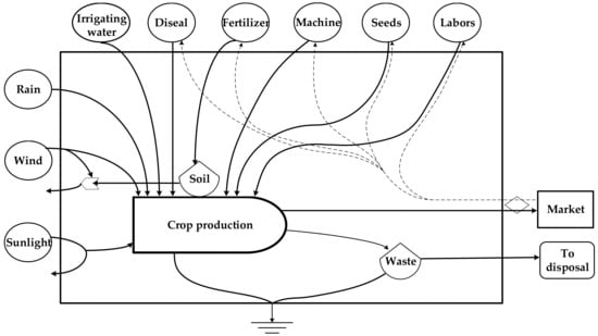
Figure 1.
Emergy flow diagram of a Chinese crop system.
2.2.2. Computational Table and Characteristic Coefficients
Based on a distinct diagram, a computational table is designed to categorize different input flows according to their characteristics and to allow their conversions from conventional units (energy and exergy, Joule (J); mass, gram (g); labor or services, hour (h).) into solar emergy Joule (sej). The amount of input emergy of the solar kind invested per reference (or functional) unit is named unit emergy value (UEV) and measured as the solar equivalent Joule per unit (sej j−1; sej g−1; sej ha−1; sej h−1.). It can measure different “energy qualities” of various matters, energies, services, and information. Then, the emergy flow calculated based on the conventional unit and corresponding UEV is shown in Equation (1),
where Em represents the solar emergy of different flow (sej); fi represents the ith input flow of matter or energy (J or g); and UEVi represents the unit emergy value of ith flow (sej j−1; sej g−1). The raw flows, units, corresponding UEVs, and references of China’s crop production are listed in Table 1, which is referenced by an published work [30].

Table 1.
Emergy flows and corresponding unit emergy values (UEVs) in China.
2.2.3. Emergy-Based Indicators
In general, all the inputs of such a crop production system can be classified into three types: (1) local renewable resources (R) such as sunlight, earth cycle; (2) local non-renewable resources (N) such as the net loss of the topsoil; (3) purchased resources (F) such as mechanical equipment, purchased diesel, chemical fertilizers, pesticides, and labor (L). Labor represents the human resources used in the support of crop production and is an essential component of purchased resources (F). Thus, the total emergy input of one crop production system (U) can be expressed as Equation (2),
where U represents the total emergy used (sej); R is the renewable resource emergy (sej); N is the non-renewable resource emergy (sej); and F is the purchased resource emergy (sej).
Subsequently, three commonly used emergy indicators, namely the emergy yield ratio (EYR), environmental load ratio (ELR), and ESI, are employed to evaluate the yield, environmental load, and sustainability of China’s crop production system based on the aggregated emery flows of R, N, F, and U.
- (1)
- EYR
EYR is the ratio of the total emergy used (U) divided by the purchased resources emergy (F). It is an indicator of the yield compared with inputs other than local inputs and gives a measure of the ability of the process to exploit local resources accounting for the difference between local and imported [36]. If the value equals 1 or is only slightly higher than 1, it means that this system consumes less new local resources than those that were available as inputs for the system’s growth [37]. The higher this ratio is, the more dependent it is on local resources exploitation or is less dependent on outside resources. The EYR is expressed as Equation (3),
where EYR represents the emergy yield ratio; U is the total emergy used (sej); and F is the purchased resources emergy (sej).
- (2)
- ELR
ELR is the ratio of locally non-renewable resources (N) and purchased resources emergy (F) to the local renewable resources emergy (R), which measures the environmental pressure resulting from the use of all non-renewable resources (N and F). It is an indicator of addressing the pressure of agricultural production on the local ecosystem and can measure ecosystem stress due to crop production [37]. The smaller the ELR is, the less environmental pressure it has on the local natural system. Unlike EYR, which evaluates the balance between imported and local resources, ELR measures the balance between renewable and non-renewable resources, which expressed as Equation (4),
where ELR represents the environmental loading ratio; N + F is the non-renewable resources emergy (sej); and R is the locally renewable resources emergy (sej).
- (3)
- ESI
ESI is the ratio of EYR to ELR, which takes both ecological and economic perspectives into account. To be more specific, a lower ESI value (such as less than 1) is indicative of a highly developed consumer-oriented economy, while a higher ESI value (more than 10) is indicative of an undeveloped economy with abundant local resources. An ESI value between 1 and 10 is indicative of one developing economy [36], expressed as Equation (5),
where ESI represents the emergy sustainability index; EYR is the emergy yield ratio; and ELR represents the environmental loading ratio.
2.3. The Decomposition Analysis Method (LMDI)
There are two key emergy-based indicators for assessing crop production, namely the total emergy used (U) and ESI. To raise appropriate long-term development strategies, it is not sufficient to merely study the variation trend of U and ESI. Thus, the key driving forces affecting the change of indicators should be identified so that the extent of positive or negative contribution can be quantified, and targeted policies and suggestions can be raised. First, such work requires the establishment of two decomposition formulas, which is the basis and premise of applying a decomposition analysis.
The equation for describing the relationship among the contribution of different factors to a variable U can be expressed by Equation (6):
where U/F is the EYR; F/(R + N) is the emergy investment ratio (EIR), the indicator which measures the efficiency of the external investment in exploiting a unit of local resources; (R + N)/GDP is the local emergy (sej ¥−1) measuring the local resources consumption based on a unit of agricultural GDP; GDP/A is the economic output density (¥ m−2); and A is the sown area for crop production (m2).
Equation (7) describes the relationship among the contribution of different factors to a variable ESI, as below:
where U/L represents the labor resources factor, referring to the contribution of direct human labor emergy for the total emergy. The higher this ratio is, the higher the resources used per unit labor applied; L/A represents the land use factor, presenting the density of human labor per sown area (sej m−2); A/(N + F) represents the inverse measurement of non-renewable density (m sej−2), which can reflect the use intensity of non-renewable resources; R/GDP represents the renewable resources factor, referring to the intensity of local renewable resources (sej ¥−1); GDP/F represents the investment profit (¥ sej−1), indicating the whole economic yield when the system purchases resources from outside the boundary, namely the economic value generated per unit of investment from an external source.
After the establishment of the two decomposition formulas, an appropriate decomposition analysis method is needed to be chosen for further analysis. Generally, there are two major decomposition analysis methods: Structure Decomposition Analysis (SDA) and Index Decomposition Analysis (IDA). SDA is employed based on the Input-Output table, which is capable of quantifying fundamental “sources” of changes in a wide range of variables including economic growth, energy use, material intensity of use, and pollution emissions [38]. IDA focuses on both sectoral or regional level data, therefore, it is easier to interpret results and collect data [39]. The LMDI is one of the IDA methods. Compared with the Laspeyres Index Method (another commonly used IDA method), it has a specific advantage as the replacing of the zero value by a small positive number would give satisfactory decomposition results and without residual terms. The additive and multiplicative forms are two forms for applying the LMDI method [40]. For this study, the additive form was adopted with the major decomposition Formulas (8)–(14) as follows,
where M represents the values of U and ESI; Mt and M0 represent the targeted and base year, respectively; α, β, γ, δ, and ε represent the five driving factors for the U or ESI index, respectively; ΔMα, ΔMβ, ΔMγ, ΔMΔ, and ΔMε represent the contribution values of five driving forces factors for U and ESI, respectively; and ΔMrsd represents the residual (here, ΔMrsd = 0).
2.4. Data Sources
In this study, a great deal of input and output data were collected from statistical yearbooks, governmental reports, and the relevant emergy database. The raw data of input and output flows including local renewable and non-renewable resources, irrigating water, seeds, chemical, fertilizers, diesel, machineries, and agricultural GDP during the period 1997–2016 were gathered from China Statistic Yearbooks (1998–2017) [41] and China Rural Statistic Yearbooks (1998–2017) [1]. The data of average annual precipitation were gathered from the China Water Resources Bulletin (1997–2016) [42] published by the Ministry of Water Resources of the People’s Republic of China. In addition, to verify the data, some interviews with different stakeholders were conducted such as agricultural officers, farmers, and non-governmental organizations. These additional interviews played a key role in improving the accuracy of the data and ensuring the quality of the related information. The UEVs of input flows were mainly referenced by published studies and the national environmental accounting database (NEAD). According to an updated planetary emergy baseline of 1.58 × 1025 sej year−1, all the UEVs calculated prior to 2000 were multiplied by 1.68 for this study [31].
3. Results and Discussion
3.1. Total Emergy Used and Its Compositions of Chinese Crop System from 1997 to 2016
As shown in Figure 2a, the emergy flow R increased from 1.75 × 10²³ sej in 1997 to 2.07 × 10²³ sej in 2016 with a fluctuation trend during this period that was caused by the variation of annual precipitation amount and sown area. From Figure 2b, the emergy flows N were relatively stable, ranging from 3.72 × 10²² to 3.81 × 10²² sej during the period of 1997–2008. After 2008, it showed a growing trend that increased from 3.87 × 10²² in 2009 to 4.07 × 10²² sej in 2016 because of the enlargement of arable land. As seen from Figure 2c, the emergy flows L slowly increased during the period of 1997–2002 but decreased by 40.6% from 1.94 × 10²² in 2003 to 1.15 × 10²² sej in 2016, with an annual average value of −3.93%, which can be attributed to the reduction in the number of laborers engaged in crop production. Figure 2d shows that emergy flow F increased by 62.4% from 5.69 × 10²³ in 1997 to 9.24 × 10²³ sej in 2016 and emergy flow U increased by 50.0% from 7.82 × 10²³ in 1997 to 1.17 × 1024 sej in 2016. Both showed growth year by year and had a similar growing trend, with annual growth rates of 2.6% and 2.2%, respectively, which indicates that the growth trend of U is basically dependent on the variation of F.
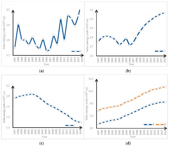
Figure 2.
The emergy flows of China’s crop production system from 1997 to 2016: (a) the variation trend of renewable resources (R); (b) the variation trend of non-renewable resources (N); (c) the variation trend of labors (L); (d) the variation of purchased resources (F) and the total emergy used (U).
Figure 3 clearly shows that emergy flow F had the largest share of the total emergy input, increasing from 70.5% in 1997 to 77.9% in 2016, so that emergy flow U is dependent on the variation of F, which was mainly derived from fertilizers, next to mechanical equipment, diesel, and pesticides, and finally from plastic mulch. Although the absolute value of R and N did not obviously decrease, the share of emergy flow R and N showed a declining trend as the growth rate of F far exceeded the growth rate of R and N, leading to a sharp increase in denominator U year by year. The share of L decreased by 58.3% from 1997 to 2016, which indicated that less and less of the labor force was engaged in crop production, owing to the urbanization trend where more and more young people choose to work and live in a town or city, instead of engaging in crop production as before. The detailed emergy flows data used in the Figure 2 and Figure 3 were can be found in Table A1 and Table A2 of Appendix A.
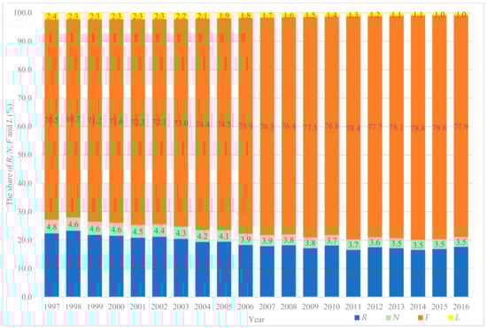
Figure 3.
The share of renewable resources (R), non-renewable resources (N), purchased resources (F) and labor (L) of China’s crop production during the period of 2007–2016.
3.2. The Results of EYR, ELR, and ESI Indicators
As shown in Figure 4, the values of EYR decreased by 8% with a fluctuating trend from 1.38 in 1997 to 1.27 in 2016, with an annual decline rate of 0.4% during the investigated period. It indicates that the ratio of (R + N)/F showed a decreasing trend (here, EYR can be further decomposed into EYR = (R + N + F)/F = (R + N)/F + 1) as a whole as the growth rate of F was further beyond (R + N). During the investigated years, the EYR values were all less than 2, indicating that the largest fraction of emergy used to generate yield was invested from outside the system to drive the process, and the system was more dependent on purchased resources, rather than on local resources. The value of ELRs ascended by 35.4% along a fluctuating trend from 3.39 in 1997 to 4.59 in 2016, with an annual growth rate of 1.6% during the investigated period. This shows that there exists a huge environmental pressure on the local ecosystem due to the transformation from traditional agriculture to modern agriculture. Unlike past crop production systems, which were very self-reliant though had low yields per hectare, modern agriculture increasingly requires huge investments from the main economy in the form of electricity, fertilizers, fuel, etc., thus leading to the overload of the local ecological capacity. As a consequence of declining EYR and increasing ELR, the value of ESIs showed a declining trend, decreasing by 9% from 1.38 in 1997 to 1.27 in 2016. The value of ESIs were all smaller than 1, still at a very low level, indicating that China’s crop production system is undergoing an unsustainable development pattern. The lower this index is, the more an economy relies on non-renewable resources and adds imports and environmental load. As it relates to economy, a low ESI (<1) is indicative of a highly developed consumer-oriented system; however, in the long run, it is not a sustainable development pattern as it unlimitedly pursues higher yield without balancing the relationship between imported resources and locally resources exploitation.
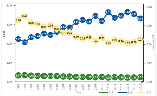
Figure 4.
The variation trend of emergy yield ratio (EYR), environment loading ratio (ELR), and emergy sustainability index (ESI) of China’s crop production system from 1997 to 2016.
3.3. Decomposition of Total Emergy U
The time changes of the amount of total emergy flow (U) were decomposed to obtain the change of five driving factors as shown in Table 2. Table 2 is divided into four sections. In the first and third sections, the values of the five factors are shown during the period of 1997–2016. In the second and fourth sections, the percentage of positive or negative contribution of each factor to the total emergy use are displayed during the investigated years. As shown in Figure 5, the results of decomposition U can be divided into two stages based on each factor’s yearly variation. During the first period from 1998 to 2004, the EYR made a negative contribution to U (except in 1998) and gradually decreased except for 2001. Compared with the EYR value in 1997, it showed that the EYR values decreased from 1.36 in 1999 to 1.31 in 2014 year by year, so the contribution percentage of EYR demonstrated a declining trend. The EIR made a positive contribution (except in 1998) and gradually increased except for 2001. It was also the maximum contributor, which indicated that a higher outside resource investment was continually required to exploit a unit of local resource. Furthermore, investments F contributed to a large extent to increase the total emergy use. The factor (R + N)/GDP acted as a positive contributor from 1998–2000 but made a negative contribution during the period of 2001–2004, which indicated that the exploitation and use of local resources lagged farther behind the economic yield after 2000. The GDP/A made a positive contribution (except in 2000) because the GDP in 2000 was less than in 1997, resulting in a lower ratio of GDP to A in 2000. The factor A made a negative contribution to total emergy U in 2003 and 2004 due to the reduction in the sown area compared with 1997. Besides these two years, all of factor A performed as a positive contributor, indicating that the sown area in China kept increasing when compared to 1997. It is easy to see that the total emergy U is linearly dependent on the A trend, indicating the vital role of factor A in affecting the change of U.
Table 2.
The contribution percentage of five driving forces for the total emergy used (U) during 1997–2016.

Figure 5.
Decomposition analysis of U during two stages: (a) Result of the five driving forces factors (EYR, emergy investment ratio (EIR), local emergy density ((R + N)/GDP), economic output density (GDP/A), and sown area (A)) of U during 1998–2004; (b) Result of driving forces of U from 2005–2016.
The variation trend of driving force factors in the second stage is summarized from 2005 to 2016. Compared to the first stage, the variation trend in the second stage can be clearly distinguished from Figure 5b. During this period, all the maximum positive and negative contributors were GDP/A and (R + N)/GDP, respectively, and generally showed a growing trend along an oscillation way, showing that the economic intensity of the per sown area was increased by technological improvement and a higher production efficiency. The EYR, acting as a negative contributor, made less contribution to total emergy U than factor (R + N)/GDP. Except for the years 2006 and 2007, factor A made a positive contribution, but rather less to total emergy U. The reduction in the sown area was responsible for acting as a negative contributor in 2006 and 2007. Finally, all EIR made a negative contribution in a fluctuation way during the second stage. Compared with the first stage (1997–2004), the positive or negative contribution of each factor during the second stage manifested as being similar, coupling with a certain changing trend. However, it was quite difficult to find a similar variation trend in the first stage, especially for 1998 as the amount of precipitation was more than in the other years, which resulted in a huge number of renewable resources.
3.4. Decomposition of Indicator ESI
As seen from Figure 4, all the ESI values were less than the year of 1997, except for 1998, accompanied by a decreasing trend during this period. According to the variation trend of positive or negative contributors shown in Table 3, the driving forces of indicator ESI can be divided into three development stages. The first development stage was from 1998–2000 shown in Figure 6a, where the factors R/GDP, L/A, and U/L played a role in promoting ESI, while A/(N + F) and GDP/F acted as restricting factors for ESI growth. In 1998, the overall effect of the five indicators was positive as the renewable resources were large because of the huge precipitation and relatively slow GDP growth in crop production, leading to a larger positive contribution from factor R/GDP and smaller negative contribution from GDP/F. As shown in Figure 6b, the second stage from 2001 to 2004 was a little different from the first stage, where factor R/GDP changed from positive to negative, indicating that the growth of GDP for crop production was built on the overload of the environmental capacity, thus aggravating the extent of an unsustainable pattern. The last stage experienced a long time, from 2005 to 2016, as shown in Figure 6c. There were two distinguished changes during this period where positive contributor L/A became negative and the simultaneously negative contributor GDP/F acted as a positive one, completely opposite to the first two stages. This phenomenon indicates that the improvement of resource efficiency played a vital role in promoting the sustainable production pattern, while decreasing the number of laborers who were already engaged in crop production impeded the sustainable development of China’s crop production with an increasing negative contribution percentage of L/A year by year, which verified the research findings from Xu [43] and Yu [44] that urbanization and technological advancement were two key factors affecting the sustainability of agriculture. In summary, there were more positive contributors in the first stage than in the second and third stages. As per an increasing number of negative contributors, the indicator ESI showed a gradually decreasing trend after the first period, indicating a decline in the sustainable level of China’s crop production.
Table 3.
The contribution values of five driving forces for ESI from 1997 to 2016.
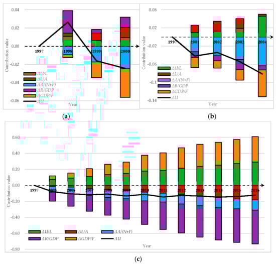
Figure 6.
Decomposition analysis of indicator ESI during three stages: (a) Driving forces factors (the ratio of total emergy used to labor (U/L), the ratio of labor to sown area (L/A), the ratio of sown area to non-renewable resources A/(N + F), the ratio of renewable resources to gross domestic products (R/GDP), the ratio of gross domestic products to purchased resources GDP/F of ESI during 1998–2000); (b) Driving forces of ESI during 2001–2004; (c) Driving forces of ESI during 2005–2016.
4. Conclusions and Policy Implications
China’s crop production system is undergoing unsustainable development due to the ever-increasing environmental stress caused by a large consumption of non-renewable resources. To seek region-specific mitigation policies, it is necessary to evaluate the overall performance of China’s crop production. Under such circumstances, this study first employed the emergy method to make a time series analysis of performance for China’s crop production so that the composition and variation trend of U and ESI were obtained during the period of 1997–2016. Next, the U and ESI were respectively decomposed into five driving force factors to further identify the contribution values for these factors in affecting the change of U and ESI. The main findings are summarized as follows:
- (1)
- From 1997 to 2016, the U increased by 50% from 7.82 × 10²³ to 1.17 × 1024 sej with an annual average growth rate of 2.2%, which was basically dependent on the variation trend of F. That is to say, many purchased resources with a higher energy hierarchy (UEVs) including fertilizers, mechanical equipment, diesel, and pesticides are used to satisfy crop demands. During the first stage from 1997 to 2004, the largest positive contributor (contribution percentage: more than 70%) was derived from factor EIR, but factor GDP/A (more than 200%) became the maximum contributor during the second stage from 2005 to 2016, which showed that the economic intensity per sown area increased through technological improvement and higher production efficiency. Therefore, raising the efficiency of agricultural supplies is a valid way for reducing the emergy of non-renewable inputs.
- (2)
- During the investigated period, the values of ESI were all smaller than 1 with a declining trend, which was attributed to the relatively stable EYR values and continuously increasing ELR values. From the results of the ESI decomposition analysis, factor R/GDP made a negative contribution to ESI after 2000, indicating that the renewable resources capacity of per GDP decreased. If the renewable resources capacity is improved, the value of ESI will be promoted simultaneously. If there are more renewable electricity, heat, biomaterials, biofuels, fertilizers, this would entail a decreased amount of F and N emergy. This suggests greater efforts in recovering local ecosystems so that ecosystem service can be enhanced.
- (3)
- The decomposition analysis of ESI showed that factor L/A made a positive contribution to ESI from 0.0036 in 1998 to 0.0045 in 2004 and made negative contributing values from −0.0143 in 2005 to −0.1821 in 2016, which indicated that the laborers per unit of arable land declined after 2004 when compared with the base year. Therefore, the number of farmers became the impeding factor for the sustainability of crop production. Effective measures should be adopted to prevent the reduction of farmers. Regional cooperation is necessary so that more advanced technologies can be transferred from those developed areas to less developed areas. Thus, the national governments should facilitate greater regional coordination through technological transfer, capacity-building aids, and financial support to attract more young people to engage in crop production.
- (4)
- To simplify the calculations, this study used those transformations published in different journals and international databases. Although such treatment may not guarantee accuracy, it can at least present the basic development trends of China’s crop production. In the future, it will be necessary to conduct further regional studies so that more accurate transformations can be obtained for more accurate analysis. Furthermore, the economic and environmental performances of the farm-scale will be studied to obtain the sustainable development level of China’s farms by emergy analysis in future work.
Author Contributions
Conceptualization, Z.L.; Data curation, R.L. and T.Y.; Formal analysis, Y.W.; Investigation, J.G.; Project administration, S.W.; Writing—review and editing, H.D., Y.G., and B.X.
Funding
This research was funded by [natural science foundation of Liaoning province] grant number [20180550435], [national science foudation of China] grant number [41471116] and [the education department of Liaoning fund] grant number [L201609].
Acknowledgments
Thanks for two anonymous reviewers and all the editors in the process of revision.
Conflicts of Interest
The authors declare no conflict of interest.
Appendix A
Table A1.
The emergy inputs flows of China crop production system during the period of 199–2016.
Table A1.
The emergy inputs flows of China crop production system during the period of 199–2016.
| No | Item | Units | 1997 | 1998 | 1999 | 2000 | 2001 | 2002 | 2003 | 2004 | 2005 | 2006 |
|---|---|---|---|---|---|---|---|---|---|---|---|---|
| Local renewable resources (R) | ||||||||||||
| 1 | Sunlight | J | 5.54 × 10²¹ | 5.60 × 10²¹ | 5.63 × 10²¹ | 5.62 × 10²¹ | 5.60 × 10²¹ | 5.56 × 10²¹ | 5.48 × 10²¹ | 5.53 × 10²¹ | 5.60 × 10²¹ | 5.48 × 10²¹ |
| 2 | Wind, (kinetic energy) | J | 9.32 × 10²¹ | 9.42 × 10²¹ | 9.46 × 10²¹ | 9.46 × 10²¹ | 9.42 × 10²¹ | 9.36 × 10²¹ | 9.22 × 10²¹ | 9.29 × 10²¹ × | 9.41 × 10²¹ | 9.21 × 10²¹ |
| 3a | Rain (chemical potential energy) | J | 8.56 × 10²² | 1.01 × 10²³ | 8.92 × 10²² | 8.97 × 10²² | 8.64 × 10²² | 9.26 × 10²² | 8.82 × 10²² | 8.50 × 10²² | 9.09 × 10²² | 8.43 × 10²² |
| 3b | Rain (Geopotential energy) | J | 2.30 × 10²² | 2.70 × 10²² | 2.39 × 10²² | 2.41 × 10²² | 1.63 × 10²² | 2.48 × 10²² | 2.37 × 10²² | 2.28 × 10²² | 2.44 × 10²² | 2.26 × 10²² |
| 4 | Earth Cycle | J | 8.93 × 10²² | 9.03 × 10²² | 9.07 × 10²² | 9.07 × 10²² | 9.03 × 10²² | 8.97 × 10²² | 8.84 × 10²² | 8.91 × 10²² | 9.02 × 10²² | 8.82 × 10²² |
| Local non-renewable resources (N) | ||||||||||||
| 5 | Net loss of topsoil | g | 3.76 × 10²² | 3.80 × 10²² | 3.81 × 10²² | 3.81 × 10²² | 3.80 × 10²² | 3.77 × 10²² | 3.72 × 10²² | 3.75 × 10²² | 3.79 × 10²² | 3.71 × 10²² |
| Purchased renewable resources (F) | ||||||||||||
| 6 | Irrigating water | J | 1.46 × 10²² | 1.42 × 10²² | 1.44 × 10²² | 1.40 × 10²² | 1.41 × 10²² | 1.37 × 10²² | 1.39 × 10²² | 1.45 × 10²² | 1.45 × 10²² | 1.48 × 10²² |
| 7 | Seeds | J | 1.05 × 10²³ | 1.06 × 10²³ | 1.07 × 10²³ | 1.07 × 10²³ | 1.06 × 10²³ | 1.05 × 10²³ | 1.04 × 10²³ | 1.05 × 10²³ | 1.06 × 10²³ | 1.04 × 10²³ |
| 8 | Human labor (L) | J | 1.84 × 10²² | 1.88 × 10²² | 1.91 × 10²² | 1.93 × 10²² | 1.95 × 10²² | 1.96 × 10²² | 1.94 × 10²² | 1.86 × 10²² | 1.79 × 10²² | 1.71 × 10²² |
| 9 | Mechanical equipment | g | 1.16 × 10²³ | 1.25 × 10²³ | 1.35 × 10²³ | 1.46 × 10²³ | 1.49 × 10²³ | 1.54 × 10²³ | 1.58 × 10²³ | 1.69 × 10²³ | 1.81 × 10²³ | 1.93 × 10²³ |
| 10 | Diesel | J | 7.03 × 10²² | 7.52 × 10²² | 7.74 × 10²² | 8.03 × 10²² | 8.49 × 10²² | 8.62 × 10²² | 9.00 × 10²² | 1.04 × 10²³ | 1.09 × 10²³ | 1.10 × 10²³ |
| 11 | Nitrogen fertilizer | g | 1.39 × 10²³ | 1.42 × 10²³ | 1.39 × 10²³ | 1.38 × 10²³ | 1.38 × 10²³ | 1.38 × 10²³ | 1.37 × 10²³ | 1.42 × 10²³ | 1.42 × 10²³ | 1.44 × 10²³ |
| 12 | Phosphate fertilizer | g | 4.51 × 10²² | 4.47 × 10²² | 4.57 × 10²² | 4.52 × 10²² | 4.62 × 10²² | 4.67 × 10²² | 4.68 × 10²² | 4.82 × 10²² | 4.87 × 10²² | 5.04 × 10²² |
| 13 | Potash fertilizer | g | 5.96 × 10²¹ | 6.40 × 10²¹ | 6.76 × 10²¹ | 6.97 × 10²¹ | 7.39 × 10²¹ | 7.81 × 10²¹ | 8.10 × 10²¹ | 8.64 × 10²¹ | 9.05 × 10²¹ | 9.43 × 10²¹ |
| 14 | Compound fertilizer | g | 3.75 × 10²² | 3.86 × 10²² | 4.14 × 10²² | 4.31 × 10²² | 4.62 × 10²² | 4.89 × 10²² | 5.22 × 10²² | 5.66 × 10²² | 6.12 × 10²² | 6.51 × 10²² |
| 15 | Pesticides | g | 1.77 × 10²² | 1.82 × 10²² | 1.96 × 10²² | 1.89 × 10²² | 1.89 × 10²² | 1.94 × 10²² | 1.96 × 10²² | 2.05 × 10²² | 2.16 × 10²² | 2.27 × 10²² |
| 16 | Plastic mulch | g | 4.41 × 10²⁰ | 4.59 × 10²¹ | 4.78 × 10²¹ | 5.07 × 10²¹ | 5.51 × 10²¹ | 5.82 × 10²¹ | 6.05 × 10²¹ | 6.38 × 10²¹ | 6.70 × 10²¹ | 7.01 × 10²¹ |
| No | Item | Units | 2007 | 2008 | 2009 | 2010 | 2011 | 2012 | 2013 | 2014 | 2015 | 2016 |
| Local renewable resources (R) | ||||||||||||
| 1 | Sunlight | J | 5.52 × 10²¹ | 5.62 × 10²¹ | 5.71 × 10²¹ | 5.78 × 10²¹ | 5.84 × 10²¹ | 5.88 × 10²¹ | 5.92 × 10²¹ | 5.95 × 10²¹ | 5.99 × 10²¹ | 6.00 × 10²¹ |
| 2 | Wind, (kinetic energy) | J | 9.29 × 10²¹ | 9.46 × 10²¹ | 9.60 × 10²¹ | 9.72 × 10²¹ | 9.82 × 10²¹ | 9.89 × 10²¹ | 9.96 × 10²¹ | 1.00 × 10²² | 1.01 × 10²² | 1.01 × 10²² |
| 3a | Rain (chemical potential energy) | J | 8.49 × 10²² | 9.28 × 10²² | 8.50 × 10²² | 1.01 × 10²³ | 8.57 × 10²² | 1.02 × 10²³ | 9.88 × 10²² | 9.34 × 10²² | 9.97 × 10²² | 1.10 × 10²³ |
| 3b | Rain (Geopotential energy) | J | 2.28 × 10²² | 2.49 × 10²² | 2.28 × 10²² | 2.72 × 10²² | 2.30 × 10²² | 2.74 × 10²² | 2.65 × 10²² | 2.51 × 10²² | 2.68 × 10²² | 2.96 × 10²² |
| 4 | Earth Cycle | J | 8.90 × 10²² | 9.06 × 10²² | 9.20 × 10²² | 9.32 × 10²² | 9.41 × 10²² | 9.48 × 10²² | 9.55 × 10²² | 9.60 × 10²² | 9.65 × 10²² | 9.67 × 10²² |
| Local non-renewable resources (N) | ||||||||||||
| 5 | Net loss of topsoil | g | 3.74 × 10²² | 3.81 × 10²² | 3.87 × 10²² | 3.92 × 10²² | 3.96 × 10²² | 3.99 × 10²² | 4.02 × 10²² | 4.04 × 10²² | 4.06 × 10²² | 4.07 × 10²² |
| Purchased renewable resources (F) | ||||||||||||
| 6 | Irrigating water | J | 1.46 × 10²² | 1.48 × 10²² | 1.51 × 10²² | 1.49 × 10²² | 1.52 × 10²² | 1.58 × 10²² | 1.59 × 10²² | 1.57 × 10²² | 1.56 × 10²² | 1.53 × 10²² |
| 7 | Seeds | J | 1.05 × 10²³ | 1.07 × 10²³ | 1.08 × 10²³ | 1.10 × 10²³ | 1.11 × 10²³ | 1.11 × 10²³ | 1.12 × 10²³ | 1.13 × 10²³ | 1.13 × 10²³ | 1.14 × 10²³ |
| 8 | Human labor (L) | J | 1.64 × 10²² | 1.60 × 10²² | 1.54 × 10²² | 1.49 × 10²² | 1.42 × 10²² | 1.38 × 10²² | 1.29 × 10²² | 1.22 × 10²² | 1.17 × 10²² | 1.15 × 10²² |
| 9 | Mechanical equipment | g | 2.05 × 10²³ | 2.30 × 10²³ | 2.45 × 10²³ | 2.59 × 10²³ | 2.72 × 10²³ | 2.84 × 10²³ | 2.90 × 10²³ | 3.01 × 10²³ | 3.10 × 10²³ | 3.19 × 10²³ |
| 10 | Diesel | J | 1.16 × 10²³ | 1.08 × 10²³ | 1.12 × 10²³ | 1.16 × 10²³ | 1.18 × 10²³ | 1.20 × 10²³ | 1.23 × 10²³ | 1.24 × 10²³ | 1.26 × 10²³ | 1.21 × 10²³ |
| 11 | Nitrogen fertilizer | g | 1.47 × 10²³ | 1.47 × 10²³ | 1.49 × 10²³ | 1.50 × 10²³ | 1.52 × 10²³ | 1.53 × 10²³ | 1.53 × 10²³ | 1.53 × 10²³ | 1.51 × 10²³ | 1.47 × 10²³ |
| 12 | Phosphate fertilizer | g | 5.06 × 10²² | 5.11 × 10²² | 5.22 × 10²² | 5.28 × 10²² | 5.37 × 10²² | 5.43 × 10²² | 5.44 × 10²² | 5.54 × 10²² | 5.52 × 10²² | 5.44 × 10²² |
| 13 | Potash fertilizer | g | 9.87 × 10²¹ | 1.01 × 10²² | 1.04 × 10²² | 1.08 × 10²² | 1.12 × 10²² | 1.14 × 10²² | 1.16 × 10²² | 1.19 × 10²² | 1.19 × 10²² | 1.18 × 10²² |
| 14 | Compound fertilizer | g | 7.06 × 10²² | 7.56 × 10²² | 7.98 × 10²² | 8.45 × 10²² | 8.91 × 10²² | 9.35 × 10²² | 9.67 × 10²² | 9.94 × 10²² | 1.02 × 10²³ | 1.04 × 10²³ |
| 15 | Pesticides | g | 2.40 × 10²² | 2.48 × 10²² | 2.53 × 10²² | 2.60 × 10²² | 2.64 × 10²² | 2.67 × 10²² | 2.67 × 10²² | 2.67 × 10²² | 2.64 × 10²² | 2.58 × 10²² |
| 16 | Plastic mulch | g | 7.36 × 10²⁰ | 7.63 × 10²⁰ | 7.90 × 10²⁰ | 8.26 × 10²⁰ | 8.72 × 10²⁰ | 9.06 × 10²⁰ | 9.47 × 10²⁰ | 9.80 × 10²⁰ | 9.89 × 10²⁰ | 9.89 × 10²⁰ |
Table A2.
Emergy flows and indicators of Chines crop production system during the period of 1997–2016.
Table A2.
Emergy flows and indicators of Chines crop production system during the period of 1997–2016.
| No | Item | Units | 1997 | 1998 | 1999 | 2000 | 2001 | 2002 | 2003 | 2004 | 2005 | 2006 |
| 1 | R | sej year−1 | 1.75 × 10²³ | 1.91 × 10²³ | 1.80 × 10²³ | 1.80 × 10²³ | 1.77 × 10²³ | 1.82 × 10²³ | 1.77 × 10²³ | 1.74 × 10²³ | 1.81 × 10²³ | 1.73 × 10²³ |
| 2 | N | sej year−1 | 3.76 × 10²² | 3.80 × 10²² | 3.81 × 10²² | 3.81 × 10²² | 3.80 × 10²² | 3.77 × 10²² | 3.72 × 10²² | 3.75 × 10²² | 3.79 × 10²² | 3.71 × 10²² |
| 3 | F | sej year−1 | 5.69 × 10²³ | 5.90 × 10²³ | 6.06 × 10²³ | 6.19 × 10²³ | 6.32 × 10²³ | 6.40 × 10²³ | 6.50 × 10²³ | 6.87 × 10²³ | 7.11 × 10²³ | 7.31 × 10²³ |
| 4 | U | sej year−1 | 7.82 × 10²³ | 8.19 × 10²³ | 8.24 × 10²³ | 8.37 × 10²³ | 8.46 × 10²³ | 8.60 × 10²³ | 8.64 × 10²³ | 8.98 × 10²³ | 9.30 × 10²³ | 9.41 × 10²³ |
| 5 | L | sej year−1 | 1.84 × 10²² | 1.88 × 10²² | 1.91 × 10²² | 1.93 × 10²² | 1.95 × 10²² | 1.96 × 10²² | 1.94 × 10²² | 1.86 × 10²² | 1.79 × 10²² | 1.71 × 10²² |
| 6 | A | m2 | 1.54 × 10¹² | 1.56 × 10¹² | 1.56 × 10¹² | 1.56 × 10¹² | 1.56 × 10¹² | 1.55 × 10¹² | 1.52 × 10¹² | 1.54 × 10¹² | 1.55 × 10¹² | 1.52 × 10¹² |
| 7 | GDP | ¥ | 1.39 × 10¹² | 1.42 × 10¹² | 1.41 × 10¹² | 1.39 × 10¹² | 1.45 × 10¹² | 1.49 × 10¹² | 1.49 × 10¹² | 1.41 × 10¹² | 1.96 × 10¹² | 2.15 × 10¹² |
| 8 | EYR | – | 1.37 | 1.39 | 1.36 | 1.35 | 1.34 | 1.34 | 1.33 | 1.31 | 1.31 | 1.29 |
| 9 | ELR | – | 3.47 | 3.29 | 3.58 | 3.64 | 3.79 | 3.72 | 3.89 | 4.16 | 4.14 | 4.45 |
| 10 | ESI | – | 0.40 | 0.42 | 0.38 | 0.37 | 0.35 | 0.36 | 0.34 | 0.31 | 0.32 | 0.29 |
| 11 | EIR | – | 2.68 | 2.58 | 2.78 | 2.83 | 2.94 | 2.91 | 3.04 | 3.25 | 3.25 | 3.49 |
| 12 | (R + N)/GDP | sej ¥−1 | 1.53 × 10¹¹ | 1.61 × 10¹¹ | 1.55 × 10¹¹ | 1.58 × 10¹¹ | 1.48 × 10¹¹ | 1.47 × 10¹¹ | 1.44 × 10¹¹ | 1.50 × 10¹¹ | 1.12 × 10¹¹ | 9.73 × 10¹⁰ |
| 13 | GDP/A | ¥ m−2 | 0.90 | 0.91 | 0.90 | 0.89 | 0.93 | 0.97 | 0.98 | 0.92 | 1.26 | 1.42 |
| 14 | U/L | – | 42.40 | 43.54 | 43.09 | 43.46 | 43.49 | 43.88 | 44.63 | 48.24 | 52.04 | 42.40 |
| 15 | L/A | sej m−2 | 1.20 × 10¹⁰ | 1.21 × 10¹⁰ | 1.22 × 10¹⁰ | 1.23 × 10¹⁰ | 1.25 × 10¹⁰ | 1.27 × 10¹⁰ | 1.27 × 10¹⁰ | 1.21 × 10¹⁰ | 1.15 × 10¹⁰ | 1.12 × 10¹⁰ |
| 16 | A/(N + F) | m2 sej−1 | 2.54 × 10⁻¹² | 2.48 × 10⁻¹² | 2.43 × 10⁻¹² | 2.38 × 10⁻¹² | 2.33 × 10⁻¹² | 2.28 × 10⁻¹² | 2.22 × 10⁻¹² | 2.12 × 10⁻¹² | 2.07 × 10⁻¹² | 1.98 × 10⁻¹² |
| 17 | R/GDP | sej ¥−1 | 1.26 × 10¹¹ | 1.34 × 10¹¹ | 1.28 × 10¹¹ | 1.30 × 10¹¹ | 1.22 × 10¹¹ | 1.22 × 10¹¹ | 1.19 × 10¹¹ | 1.23 × 10¹¹ | 9.23 × 10¹¹ | 8.01 × 10¹¹ |
| 18 | GDP/F | ¥ sej−1 | 2.43 × 10⁻¹² | 2.41 × 10⁻¹² | 2.33 × 10⁻¹² | 2.24 × 10⁻¹² | 2.29 × 10⁻¹² | 2.33 × 10⁻¹² | 2.29 × 10⁻¹² | 2.06 × 10⁻¹² | 2.76 × 10⁻¹² | 2.95 × 10⁻¹² |
| No | Item | Units | 2007 | 2008 | 2009 | 2010 | 2011 | 2012 | 2013 | 2014 | 2015 | 2016 |
| 1 | R | sej year−1 | 1.74 × 10²³ | 1.83 × 10²³ | 1.77 × 10²³ | 1.95 × 10²³ | 1.80 × 10²³ | 1.97 × 10²³ | 1.94 × 10²³ | 1.89 × 10²³ | 1.96 × 10²³ | 2.07 × 10²³ |
| 2 | N | sej year−1 | 3.74 × 10²² | 3.81 × 10²² | 3.87 × 10²² | 3.92 × 10²² | 3.96 × 10²² | 3.99 × 10²² | 4.02 × 10²² | 4.04 × 10²² | 4.06 × 10²² | 4.07 × 10²² |
| 3 | F | sej year−1 | 7.59 × 10²³ | 7.85 × 10²³ | 8.13 × 10²³ | 8.39 × 10²³ | 8.63 × 10²³ | 8.86 × 10²³ | 8.98 × 10²³ | 9.13 × 10²³ | 9.24 × 10²³ | 9.24 × 10²³ |
| 4 | U | sej year−1 | 9.70 × 10²³ | 1.01 × 1024 | 1.03 × 1024 | 1.07 × 1024 | 1.08 × 1024 | 1.12 × 1024 | 1.13 × 1024 | 1.14 × 1024 | 1.16 × 1024 | 1.17 × 1024 |
| 5 | L | sej year−1 | 1.64 × 10²² | 1.60 × 10²² | 1.54 × 10²² | 1.49 × 10²² | 1.42 × 10²² | 1.38 × 10²² | 1.29 × 10²² | 1.22 × 10²² | 1.17 × 10²² | 1.15 × 10²² |
| 6 | A | m2 | 1.53 × 10¹² | 1.56 × 10¹² | 1.59 × 10¹² | 1.61 × 10¹² | 1.62 × 10¹² | 1.63 × 10¹² | 1.65 × 10¹² | 1.65 × 10¹² | 1.66 × 10¹² | 1.67 × 10¹² |
| 7 | GDP | ¥ | 2.47 × 10¹² | 2.80 × 10¹² | 3.08 × 10¹² | 3.69 × 10¹² | 4.20 × 10¹² | 4.69 × 10¹² | 5.15 × 10¹² | 5.48 × 10¹² | 5.76 × 10¹² | 5.93 × 10¹² |
| 8 | EYR | – | 1.28 | 1.28 | 1.27 | 1.28 | 1.25 | 1.27 | 1.26 | 1.25 | 1.26 | 1.27 |
| 9 | ELR | – | 4.58 | 4.49 | 4.81 | 4.52 | 5.02 | 4.70 | 4.83 | 5.04 | 4.92 | 4.66 |
| 10 | ESI | – | 0.28 | 0.29 | 0.26 | 0.28 | 0.25 | 0.27 | 0.26 | 0.25 | 0.26 | 0.27 |
| 11 | EIR | – | 3.59 | 3.54 | 3.77 | 3.59 | 3.93 | 3.74 | 3.83 | 3.98 | 3.90 | 3.73 |
| 12 | (R + N)/GDP | sej ¥−1 | 8.57 × 10¹⁰ | 7.90 × 10¹⁰ | 7.01 × 10¹⁰ | 6.33 × 10¹⁰ | 5.23 × 10¹⁰ | 5.04 × 10¹⁰ | 4.55 × 10¹⁰ | 4.19 × 10¹⁰ | 4.11 × 10¹⁰ | 4.18 × 10¹⁰ |
| 13 | GDP/A | ¥ m−2 | 1.61 | 1.79 | 1.94 | 2.30 | 2.59 | 2.87 | 3.13 | 3.31 | 3.46 | 3.56 |
| 14 | U/L | – | 59.04 | 62.90 | 66.60 | 71.84 | 76.12 | 81.46 | 87.60 | 93.79 | 99.06 | 101.98 |
| 15 | L/A | sej m−2 | 1.07 × 10¹⁰ | 1.02 × 10¹⁰ | 9.74 × 10⁹ | 9.29 × 10⁹ | 8.76 × 10⁹ | 8.43 × 10⁹ | 7.85 × 10⁹ | 7.36 × 10⁹ | 7.04 × 10⁹ | 6.90 × 10⁹ |
| 16 | A/(N + F) | m2 sej−1 | 1.93 × 10⁻¹² | 1.90 × 10⁻¹² | 1.86 × 10⁻¹² | 1.83 × 10⁻¹² | 1.80 × 10⁻¹² | 1.77 × 10⁻¹² | 1.76 × 10⁻¹² | 1.74 × 10⁻¹² | 1.72 × 10⁻¹² | 1.73 × 10⁻¹² |
| 17 | R/GDP | sej ¥−1 | 7.05 × 10¹⁰ | 6.54 × 10¹⁰ | 5.75 × 10¹⁰ | 5.27 × 10¹⁰ | 4.28 × 10¹⁰ | 4.19 × 10¹⁰ | 3.77 × 10¹⁰ | 3.46 × 10¹⁰ | 3.40 × 10¹⁰ | 3.49 × 10¹⁰ |
| 18 | GDP/F | ¥ sej−1 | 3.25 × 10⁻¹² | 3.57 × 10⁻¹² | 3.79 × 10⁻¹² | 4.40 × 10⁻¹² | 4.87 × 10⁻¹² | 5.30 × 10⁻¹² | 5.74 × 10⁻¹² | 6.00 × 10⁻¹² | 6.24 × 10⁻¹² | 6.41 × 10⁻¹² |
References
- CASY. China Agriculture Statistical Yearbook, 1st ed.; China Statistical Publishing House: Beijing, China, 1998–2017; pp. 22–121. [Google Scholar]
- FAOSTAT. Available online: http://www.fao.org/faostat/en/#home (accessed on 12 August 2018).
- Li, H.; Wang, L.; Li, J.; Gao, M.; Zhang, J.; Zhang, J.; Qiu, J.; Deng, J.; Li, C.; Frolking, S. The development of China-DNDC and review of its applications for sustaining Chinese agriculture. Ecol. Model. 2017, 348, 1–13. [Google Scholar] [CrossRef]
- Zhang, X.H.; Zhang, R.; Wu, J.; Zhang, Y.Z.; Lin, L.L.; Deng, S.H.; Li, L.; Yang, G.; Yu, X.Y.; Qi, H.; et al. An emergy evaluation of the sustainability of Chinese crop production system during 2000–2010. Ecol. Indic. 2016, 60, 622–633. [Google Scholar] [CrossRef]
- Ghisellini, P.; Zucaro, A.; Viglia, S.; Ulgiati, S. Monitoring and evaluating the sustainability of Italian agricultural system. An emergy decomposition analysis. Ecol. Model. 2014, 271, 132–148. [Google Scholar] [CrossRef]
- Didaskalou, C.; Buyuktiryaki, S.; Kecili, R.; Fonte, C.P.; Szekely, G. Valorisation of agricultural waste with an adsorption/nanofiltration hybrid process: From materials to sustainable process design. Green Chem. 2017, 19, 3116–3125. [Google Scholar] [CrossRef]
- O’Toole, P.W.; Paoli, M. The contribution of microbial biotechnology to sustainable development goals: Microbiome therapies. Microb. Biotechnol. 2017, 10, 1066–1069. [Google Scholar] [CrossRef] [PubMed]
- Fodi, T.; Didaskalou, C.; Kupai, J.; Balogh, G.T.; Huszthy, P.; Szekely, G. Nanofiltration-Enabled InSitu Solvent and Reagent Recycle for Sustainable Continuous-Flow Synthesis. ChemSusChem 2017, 10, 3435–3444. [Google Scholar] [CrossRef] [PubMed]
- Macaskie, L.E.; Mikheenko, I.P.; Omajai, J.B.; Stephen, A.J.; Wood, J. Metallic bionanocatalysts: Potential applications as green catalysts and energy materials. Microb. Biotechnol. 2017, 10, 1171–1180. [Google Scholar] [CrossRef] [PubMed]
- Razali, M.; Didaskalou, C.; Kim, J.F.; Babaei, M.; Drioli, E.; Lee, Y.M.; Szekely, G. Exploring and Exploiting the Effect of Solvent Treatment in Membrane Separations. ACS Appl. Mater. Interfaces 2017, 9, 11279–11289. [Google Scholar] [CrossRef] [PubMed]
- Rinaldi, C. Food and Gastronomy for Sustainable Place Development: A Multidisciplinary Analysis of Different Theoretical Approaches. Sustainability 2017, 9, 1748. [Google Scholar] [CrossRef]
- Geng, Y.; Sarkis, J.; Ulgiati, S.; Zhang, P. Measuring China’s Circular Economy. Science 2013, 339, 1526–1527. [Google Scholar] [CrossRef] [PubMed]
- Odum, H.T. Self-organization, transformity, and information. Science 1988, 242, 1132–1139. [Google Scholar] [CrossRef] [PubMed]
- Odum, H.T. Environmental Accounting: Emergy and Environmental Decision Making, 1st ed.; John Wiley & Sons: New York, NY, USA, 1996; pp. 30–45. [Google Scholar]
- Odum, H.T. Energy Analysis of the Environmental Role in Agriculture. In Energy and Agriculture, 1st ed.; Stanhill, G., Ed.; Springer: Berlin/Heidelberg, Germany, 1984; pp. 24–51. [Google Scholar]
- Tao, J.; Fu, M.; Zheng, X.; Zhang, J.; Zhang, D. Provincial level-based emergy evaluation of crop production system and development modes in China. Ecol. Indic. 2013, 29, 325–338. [Google Scholar] [CrossRef]
- de Barros, I.; Blazy, J.M.; Rodrigues, G.S.; Tournebize, R.; Cinna, J.P. Emergy evaluation and economic performance of banana cropping systems in Guadeloupe (French West Indies). Agric. Ecosyst. Environ. 2009, 129, 437–449. [Google Scholar] [CrossRef]
- Wang, X.L.; Chen, Y.Q.; Sui, P.; Gao, W.S.; Qin, F.; Zhang, J.S.; Wu, X. Emergy analysis of grain production systems on large-scale farms in the North China Plain based on LCA. Agric. Syst. 2014, 128, 66–78. [Google Scholar] [CrossRef]
- De Barros, I.; Pacheco, E.P.; De Carvalho, H.W.L. Integrated Emergy and Economic Performance Assessments of Maize Production in Semiarid Tropics: Comparing Tillage Systems. J. Environ. Account. Manag. 2017, 5, 211–232. [Google Scholar] [CrossRef]
- Giannetti, B.F.; Ogura, Y.; Bonilla, S.H.; Almeida, C. Accounting emergy flows to determine the best production model of a coffee plantation. Energy Policy 2011, 39, 7399–7407. [Google Scholar] [CrossRef]
- Dong, X.B.; Ulgiati, S.; Yan, M.C.; Zhang, X.S.; Gao, W.S. Energy and Emergy evaluation of bioethanol production from wheat in Henan Province, China. Energy Policy 2008, 36, 3882–3892. [Google Scholar] [CrossRef]
- Coppola, F.; Bastianoni, S.; Ostergard, H. Sustainability of bioethanol production from wheat with recycled residues as evaluated by Emergy assessment. Biomass Bioenergy 2009, 33, 1626–1642. [Google Scholar] [CrossRef]
- Saladini, F.; Gopalakrishnan, V.; Bastianoni, S.; Bakshi, B.R. Synergies between industry and nature—An emergy evaluation of a biodiesel production system integrated with ecological systems. Ecosyst. Serv. 2018, 30, 257–266. [Google Scholar] [CrossRef]
- Baral, A.; Bakshi, B.R. Thermodynamic Metrics for Aggregation of Natural Resources in Life Cycle Analysis: Insight via Application to Some Transportation Fuels. Environ. Sci. Technol. 2010, 44, 800–807. [Google Scholar] [CrossRef] [PubMed]
- Dong, H.; Liu, Z.; Geng, Y.; Fujita, T.; Fujii, M.; Sun, L.; Zhang, L. Evaluating Environmental Performance of Industrial Park Development: The Case of Shenyang. J. Ind. Ecol. 2018, 22, 1402–1412. [Google Scholar] [CrossRef]
- Tian, X.; Geng, Y.; Ulgiati, S. An emergy and decomposition assessment of China-Japan trade: Driving forces and environmental imbalance. J. Clean. Prod. 2017, 141, 359–369. [Google Scholar] [CrossRef]
- Sun, L.; Dong, H.; Geng, Y.; Li, Z.; Liu, Z.; Fujita, T.; Ohnishi, S.; Fujii, M. Uncovering driving forces on urban metabolism—A case of Shenyang. J. Clean. Prod. 2016, 114, 171–179. [Google Scholar] [CrossRef]
- Liu, Z.X.; Dong, H.J.; Geng, Y.; Lu, C.P.; Ren, W.X. Insights into the Regional Greenhouse Gas (GHG) Emission of Industrial Processes: A Case Study of Shenyang, China. Sustainability 2014, 6, 3669–3685. [Google Scholar] [CrossRef]
- Brown, M.T.; Ulgiati, S. Emergy analysis and environmental accounting. In Encyclopedia of Energy, 1st ed.; Cleveland, C., Ed.; Academic Press: Oxford, UK, 2004; Academic Press: Oxford, UK, 2004. [Google Scholar]
- Liu, Z.; Wang, Y.; Geng, Y.; Li, R.; Dong, H.; Xue, B.; Yang, T.; Wang, S. Toward sustainable crop production in China: An emergy-based evaluation. J. Clean. Prod. 2019, 206, 11–26. [Google Scholar] [CrossRef]
- Odum, H.T. Folio #2: Emergy of Global Processes. Handbook of Emergy Evaluation, 1st ed.; University of Florida: Gainesville, FL, USA, 2000; pp. 15–40. [Google Scholar]
- Campbell, D.E.; Brandt-Williams, S.L.; Meisch, M.E.A. Environmental Accounting Using Emergy: Evaluation of the State of West Virginia, 1st ed.; US Enviromental Protection Agency (USEPA): Washington, DC, USA, 2005; pp. 102–110. [Google Scholar]
- Chen, D.; Luo, Z.H.; Webber, M.; Chen, J.; Wang, W.G. Emergy evaluation of a pumping irrigation water production system in China. Front. Earth Sci. 2014, 8, 131–141. [Google Scholar] [CrossRef]
- Lan, S.F.; Odum, H.T.; Liu, X.M. Energy flow and emergy analysis of the agroecosystem of China. Ecol. Sci. 1998, 17, 32–39. [Google Scholar]
- Brown, M.T.; Arding, J. Transformity Working Paper. Center for Wetlands, 1st ed.; University of Florida: Gainesville, FL, USA, 1991; pp. 30–45. [Google Scholar]
- Ulgiati, S.; Brown, M.T. Monitoring patterns of sustainability in natural and man-made ecosystems. Ecol. Model. 1998, 108, 23–36. [Google Scholar] [CrossRef]
- Zhang, L.M.; Geng, Y.; Dong, H.J.; Zhong, Y.G.; Fujita, T.; Xue, B.; Park, H.S. Emergy-based assessment on the brownfield redevelopment of one old industrial area: A case of Tiexi in China. J. Clean. Prod. 2016, 114, 150–159. [Google Scholar] [CrossRef]
- Deng, G.Y.; Xu, Y. Accounting and structure decomposition analysis of embodied carbon trade: A global perspective. Energy 2017, 137, 140–151. [Google Scholar] [CrossRef]
- Ang, B.; Xu, X. Tracking industrial energy efficiency trends using index decomposition analysis. Energy Econ. 2013, 40, 1014–1021. [Google Scholar] [CrossRef]
- Ang, B.W. The LMDI approach to decomposition analysis: A practical guide. Energy Policy 2005, 33, 867–871. [Google Scholar] [CrossRef]
- CSY. China Statistic Yearbook, 1st ed.; China Statistical Publishing House: Beijing, China, 1998–2017; pp. 140–180. [Google Scholar]
- CWRB. China Water Resources Bulletin, 1st ed.; China Water Power Press: Beijing, China, 1997–2016; pp. 5–20. [Google Scholar]
- Xu, C.; Chunru, H.; Taylor, D.C. Sustainable agricultural development in China. World Dev. 1992, 20, 1127–1144. [Google Scholar] [CrossRef]
- Yu, J.; Wu, J. The Sustainability of Agricultural Development in China: The Agriculture–Environment Nexus. Sustainability 2018, 10, 1776. [Google Scholar] [CrossRef]
© 2018 by the authors. Licensee MDPI, Basel, Switzerland. This article is an open access article distributed under the terms and conditions of the Creative Commons Attribution (CC BY) license (http://creativecommons.org/licenses/by/4.0/).