An Integrated Approach for Sustainable Supply Chain Management with Replenishment, Transportation, and Production Decisions


Abstract
1. Introduction
2. Literature Review
3. Model Development
3.1. Assumptions
- Demand of each part in each period is known. The production is based on make-to-order.
- There is no beginning inventory in the first period.
- Ordering lead time, purchase lead time, transportation lead time, and production lead time are known and set to zero.
- Transportation distance and the transportation loading size of each vehicle are fixed and known.
- A larger vehicle produces a higher amount of emissions.
- Each kind of part can be purchased from at least two suppliers and can be purchased from only one supplier in a period.
- Quantity discount is available. The unit-purchase cost of each kind of part is determined by the quantity of the part purchased in that period.
- The purchased amount of each kind of part must be delivered in a single batch in a period.
- The transportation of the ordered parts in a period must be complete in that period.
- At most, one vehicle can travel to and out of a shipment point (supplier) in each period.
- Products can be produced in advance, and backlogging is allowed.
- Different materials incur different amounts of emissions depending on when they were made.
- Different production modes incur different amounts of emissions.
3.2. Various Costs
3.3. Mixed Integer Programming (MIP)
3.4. Particle Swarm Optimization (PSO)
- Step 1. Initialize particles with random positions and velocities. With a search space of d-dimensions, a set of random particles (solutions) is first initialized. Let the lower and the upper bounds on the variables’ values be and . We can randomly generate the positions, (the superscript denotes the particle, and the subscript denotes the iteration), and the exploration velocities, , of the initial swarm of particles:where the positions and exploration velocities are in a vector format, rand is a random number between 0 and 1, and Δ is the constant time increment, and is assumed to be 1.
- Step 2. Evaluate the fitness of all of the particles. The performance of each solution is evaluated with the fitness function.
- Step 3. Generate initial feasible solutions.
- Step 4. Keep track of the locations where each individual has its highest fitness.
- Step 5. Keep track of the position with the global best fitness.
- Step 6. Update the velocity of each particle:where is the inertia factor, is the velocity of the particle at the iteration, and are the acceleration constants toward and , rand1 and rand2 are random numbers between 0 and 1, is the best searching experience of the particle so far at the iteration, is the best result obtained among all of the particles at the iteration, is the current position of the particle, and can be set as a constant value or a variable changing in all of the iterations.
- Step 7. Update the position of each particle:
- Step 8. Perform production planning and generate new feasible solutions ().
- Step 9. Terminate the process if a maximum number of iterations is attained. Otherwise, go to Step 2.
4. Case Studies
4.1. Data
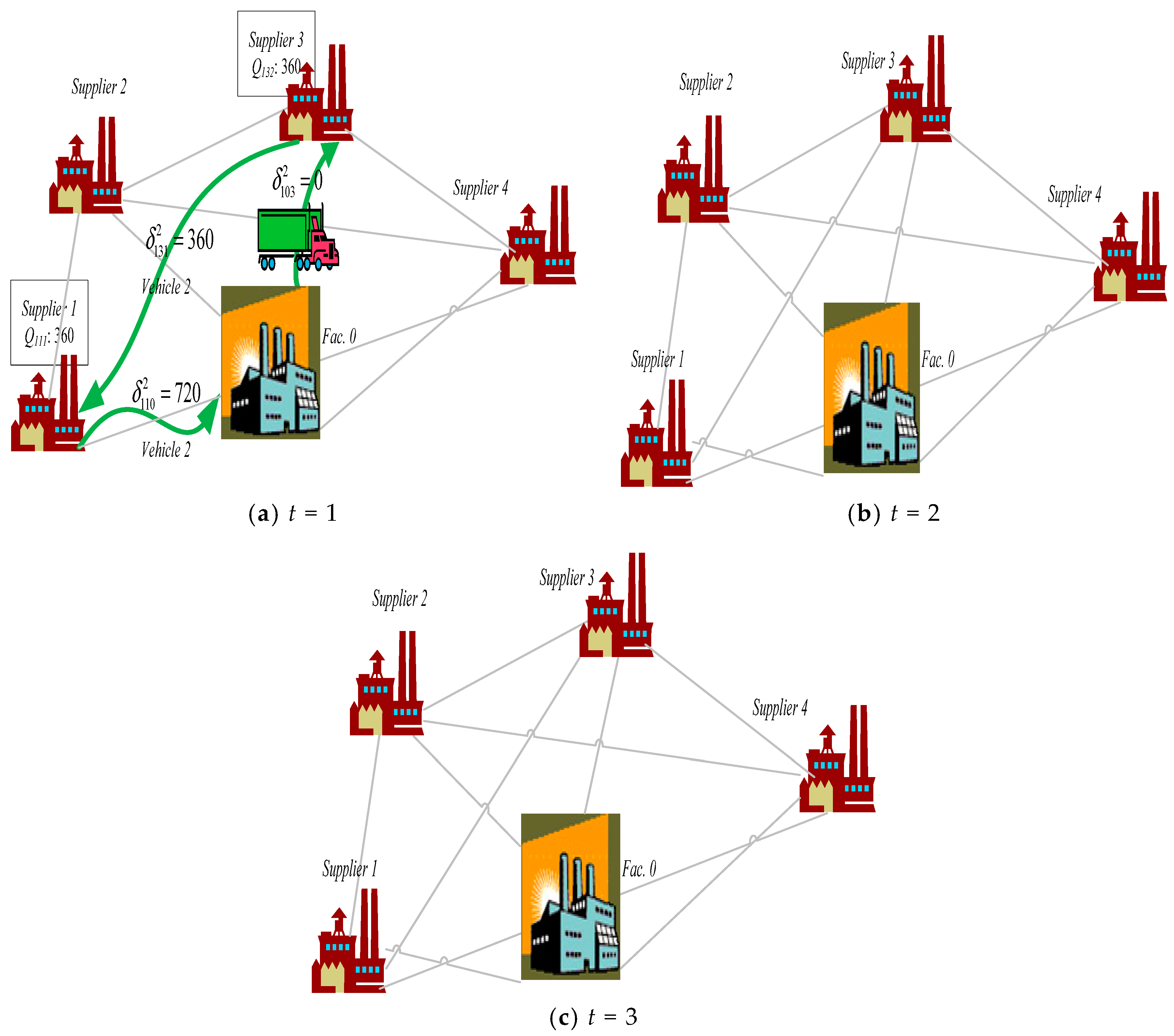
4.2. Case I
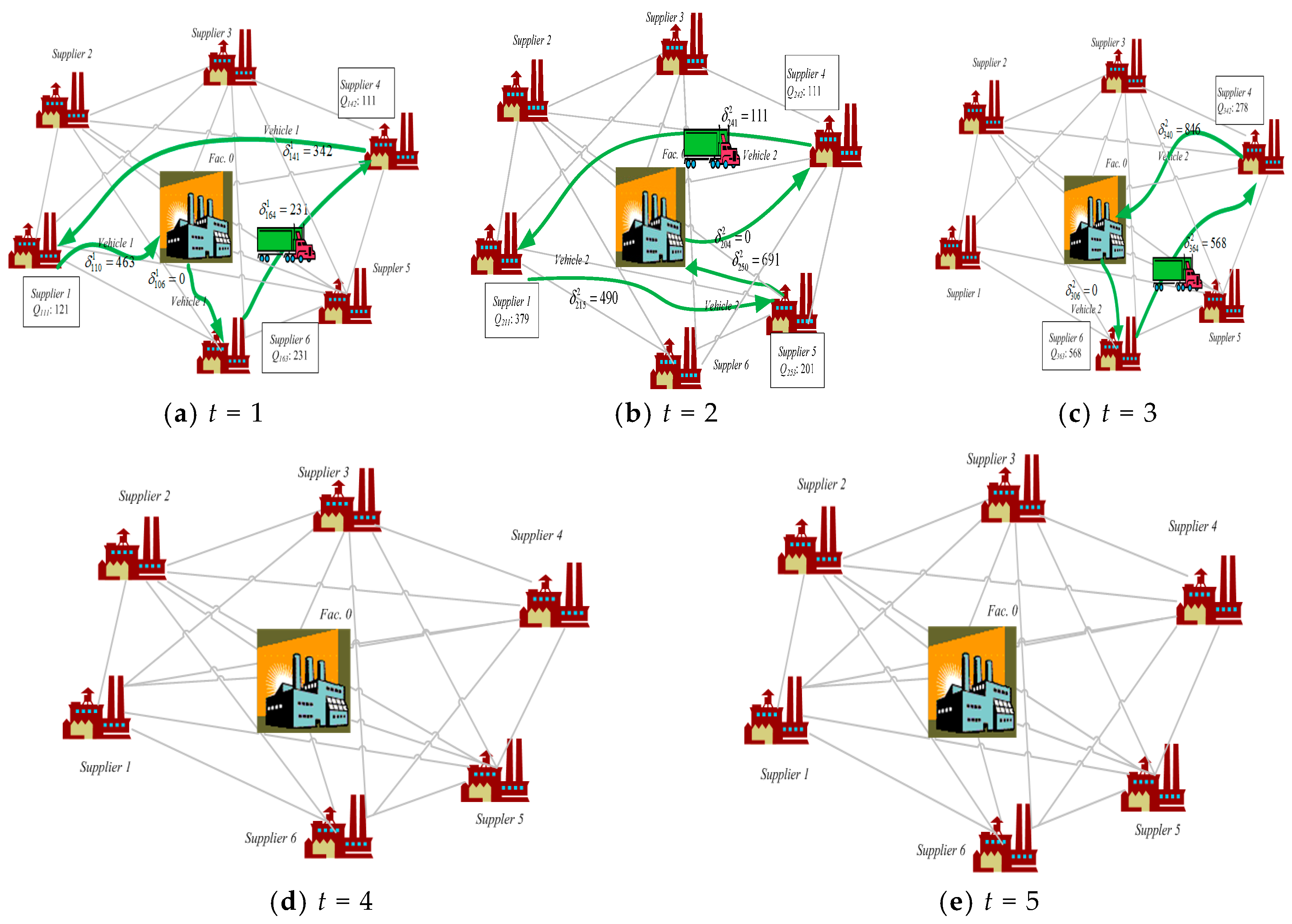
4.3. Case II
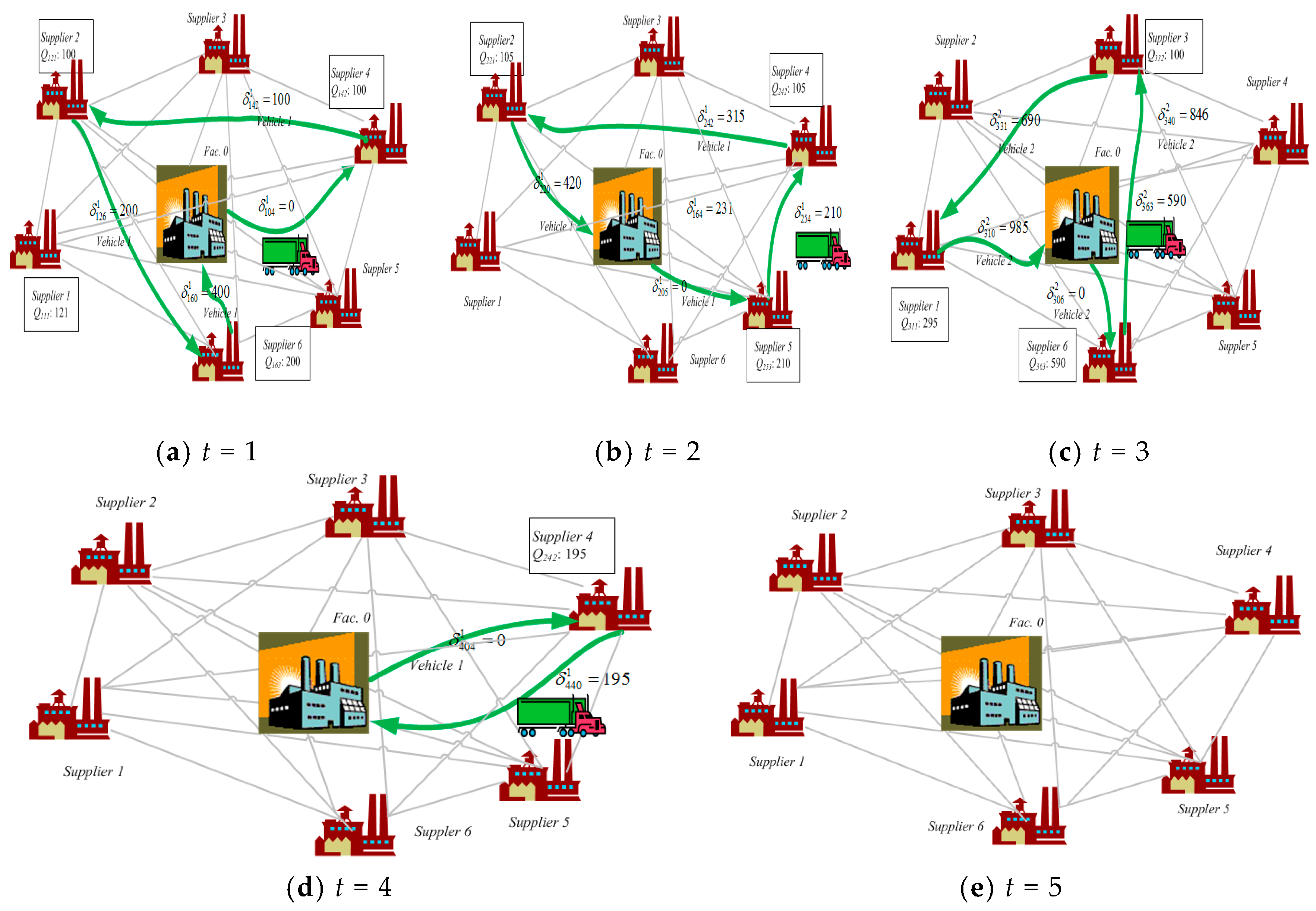
4.4. Case III
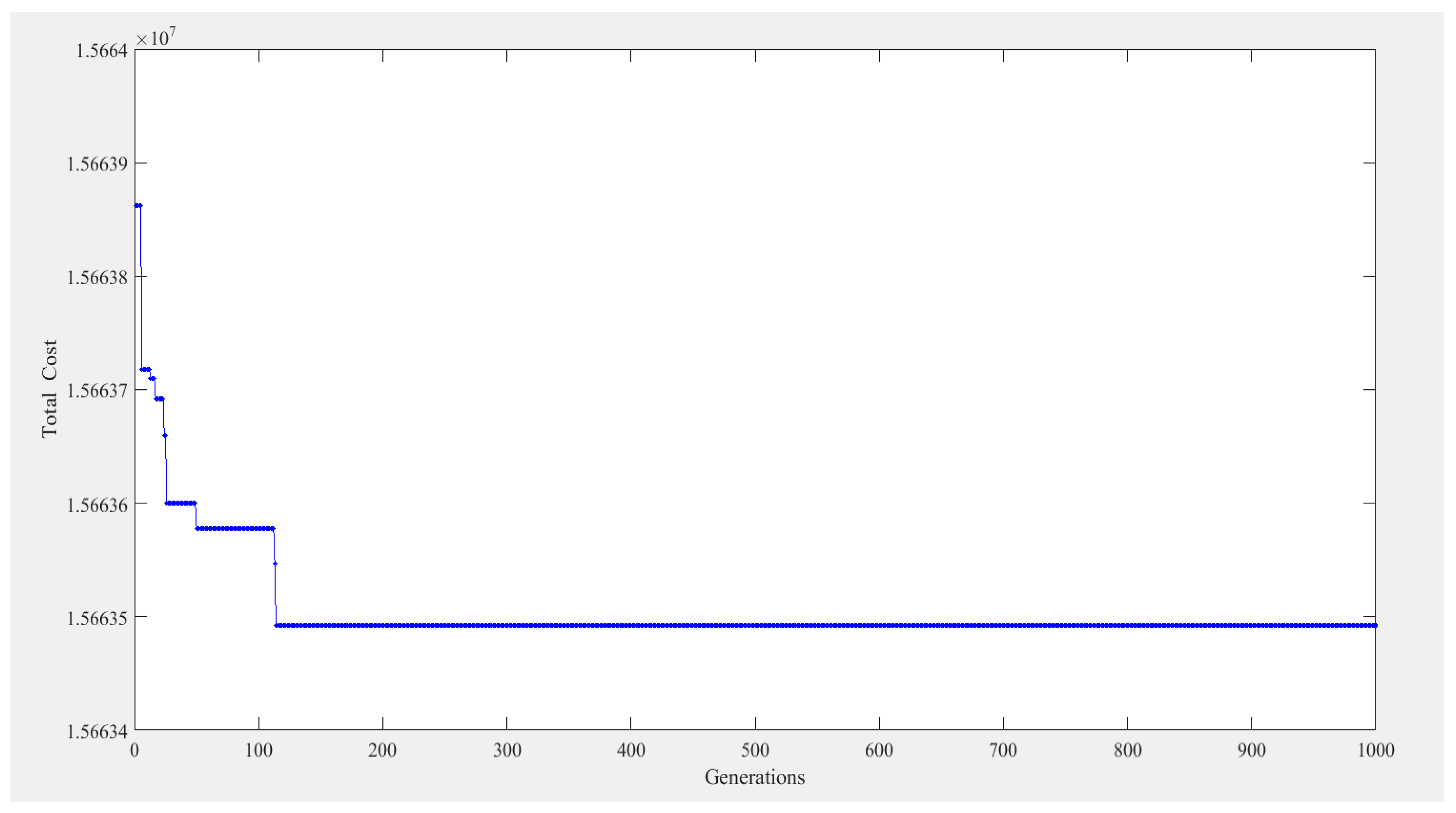
5. Results and Discussions
6. Conclusions
Author Contributions
Funding
Conflicts of Interest
Abbreviations
| Supplier (v = 1, 2, 3, …, V) | |
| Part (r = 1, 2, 3, …, R) | |
| Finished good (g = 1, 2, 3, …, G) | |
| Period (t = 1, 2, 3, …, T) | |
| Production mode (s = 1, 2, 3, …, S) | |
| Quantity discount bracket for parts (x = 1, 2, 3, …, X) | |
| Shipment point, 0 indicates factory (i = 1, 2, 3, …, I; j = 1, 2, 3, …, J) | |
| Vehicle (= 1, 2, 3, …,) |
| Demand of part r in period t | |
| Demand of finished good g in period t | |
| Ordering cost of part r from supplier v for each purchase | |
| Unit holding cost of part r per period | |
| Unit holding cost of finished good g per period | |
| Unit backlogging cost of part r per period | |
| Unit backlogging cost of finished good g per period | |
| M | A large number |
| Unit purchase cost of part r under quantity discount bracket x from supplier v in period t | |
| Maximum quantity of part r under quantity discount bracket x from supplier v | |
| Maximum accumulated quantity of finished good g that can be produced from production mode 1 to s | |
| Maximum travelling length of vehicle e | |
| Distance from shipment point i to shipment point j | |
| Maximum loading size of vehicle e | |
| Units of material r required to produce product g. | |
| Transportation cost from shipment point i to shipment point j | |
| Fixed cost of vehicle e per trip | |
| Carbon emission cost of vehicle e per distance | |
| Carbon emission cost per unit of material r | |
| Carbon emission cost per unit of product under production mode s |
| Unit purchase cost of part r from supplier v in period t | |
| Quantity of part r purchased from supplier v in period t | |
| Total quantity of part r purchased in period t | |
| Unit production cost of finished good g under production mode s in period t. Depending on the quantity manufactured, the unit production cost will be based on the production mode. | |
| Production quantity of finished good g under production mode s in period t | |
| Total quantity of finished good g produced in period t | |
| Purchase size from shipment point i in period t | |
| Loading size of vehicle e from shipment point i to shipment point j in period t | |
| Ending inventory of part r in period t | |
| Ending inventory of finished good g in period t | |
| Backlogging of part r in period t | |
| Backlogging of finished good g in period t | |
| Binary variable, 1 indicates that an order of part r from supplier v in period t is placed, and 0 indicates that no order is placed | |
| Binary variable, 1 indicates that an order of part r under quantity discount bracket x from supplier v in period t is placed, and 0 indicates that no order is placed | |
| Binary variable, 1 indicates that vehicle e travels from shipment point i to shipment point j in period t, and 0 indicates that no travel is incurred | |
| Binary variable, 1 indicates that vehicle e travels from shipment point i in period t, and 0 indicates that no travel is incurred | |
| Binary variable, 1 indicates that finished good g is manufactured under production mode s in period t, and 0 indicates that no product is manufactured |
References
- Harland, C.M. Supply chain management: Relationships, chains and networks. Br. Acad. Manag. J. 1996, 7, S63–S80. [Google Scholar] [CrossRef]
- Sadeghi, J.; Sadeghi, S.; Niaki, S.T.A. A hybrid vendor managed inventory and redundancy allocation optimization problem in supply chain management: An NSGA-II with tuned parameters. Oper. Res. 2014, 41, 53–64. [Google Scholar] [CrossRef]
- Toro, E.M.; Franco, J.F.; Echeverri, M.G.; Guimarães, F.G. A multi-objective model for the green capacitated location-routing problem considering environmental impact. Comput. Ind. Eng. 2017, 110, 114–125. [Google Scholar] [CrossRef]
- Kannan, D.; Diabat, A.; Alrefaei, M.; Govindan, K.; Yong, G. A carbon footprint based reverse logistics network design model. Resour. Conserv. Recycl. 2012, 67, 75–79. [Google Scholar] [CrossRef]
- Pan, S.; Ballot, E.; Fontane, F. The reduction of greenhouse gas emissions from freight transport by pooling supply chains. Int. J. Prod. Econ. 2013, 143, 86–94. [Google Scholar] [CrossRef]
- Sarkar, B.; Saren, S.; Sarkar, M.; Seo, Y.W. A Stackelberg game approach in an integrated inventory model with carbon-emission and setup cost reduction. Sustainability 2016, 8, 1244. [Google Scholar] [CrossRef]
- Sarkar, B.; Ganguly, B.; Sarkar, M.; Pareek, S. Effect of variable transportation and carbon emission in a three-echelon supply chain model. Trans. Res. Part E 2016, 91, 112–128. [Google Scholar] [CrossRef]
- Yuan, B.; Gu, B.; Guo, J.; Xia, L.; Xu, C. The optimal decisions for a sustainable supply chain with carbon information asymmetry under cap-and-trad. Sustainability 2018, 10, 1002. [Google Scholar] [CrossRef]
- Salehi, M.; Jalalian, M.; Siar, M.M.V. Green transportation scheduling with speed control: Trade-off between total transportation cost and carbon emission. Comput. Ind. Eng. 2017, 113, 392–404. [Google Scholar] [CrossRef]
- Soysal, M.; Çimen, M.; Demir, E. On the mathematical modeling of green one-to-one pickup and delivery problem with road segmentation. J. Clean Prod. 2018, 174, 1664–1678. [Google Scholar] [CrossRef]
- Tatsis, V.A.; Parsopoulos, K.E.; Skouri, K.; Konstantaras, I. An ant-based optimization approach for inventory routing. Adv. Intell. Syst. Comput. 2013, 227, 107–121. [Google Scholar]
- Juan, A.-A.; Grasman, S.-E.; Caceres-Cruz, J.; Bektas, T. A simheuristic algorithm for the single-period stochastic inventory-routing problem with stock-outs. Simul. Model. Pract. Theory 2014, 46, 40–52. [Google Scholar] [CrossRef]
- Ghaniabadi, M.; Mazinani, A. Dynamic lot sizing with multiple suppliers, backlogging and quantity discounts. Comput. Ind. Eng. 2017, 110, 67–74. [Google Scholar] [CrossRef]
- Kennedy, J.; Eberhart, R.C. Swarm Intelligence; Academic Press: San Diego, CA, USA, 2001. [Google Scholar]
- Jordehi, A.R.; Jasni, J. Parameter selection in particle swarm optimisation: A survey. J. Exp. Theor. Artif. Intell. 2013, 25, 527–542. [Google Scholar] [CrossRef]
- Adewumi, A.O.; Arasomwan, A.M. An improved particle swarm optimiser based on swarm success rate for global optimization problems. J. Exp. Theor. Artif. Intell. 2016, 28, 441–483. [Google Scholar] [CrossRef]
- Aminbakhsh, S.; Sonmez, R. Discrete particle swarm optimization method for the large-scale discrete time-cost trade-off problem. Expert Syst. Appl. 2016, 51, 177–185. [Google Scholar] [CrossRef]
- Liu, Z.-G.; Ji, X.-H.; Liu, Y.-X. Hybrid non-parametric particle swarm optimization and its stability analysis. Expert Syst. Appl. 2018, 92, 256–275. [Google Scholar] [CrossRef]
- Lee, A.H.I.; Kang, H.-Y.; Lai, C.-M.; Hong, W.-Y. An integrated model for lot sizing with supplier selection and quantity discounts. Appl. Math. Model. 2013, 37, 4733–4746. [Google Scholar] [CrossRef]
- Kang, H.-Y.; Lee, A.H.I. A stochastic lot-sizing model with multi-supplier and quantity discount. Int. J. Prod. Res. 2013, 51, 245–263. [Google Scholar] [CrossRef]
- Kang, H.-Y.; Pearn, W.L.; Chung, I.-P.; Lee, A.H.I. An enhanced model for the integrated production and transportation problem in a multiple vehicles environment. Soft Comput. 2016, 20, 1415–1435. [Google Scholar] [CrossRef]
- Kang, H.-Y.; Lee, A.H.I.; Wu, C.-W.; Lee, C.-H. An efficient method for dynamic-demand joint replenishment problem with multiple suppliers and multiple vehicles. Int. J. Prod. Res. 2017, 55, 1065–1084. [Google Scholar] [CrossRef]
- Darom, N.A.; Hishamuddin, H.; Ramli, R.; Mat Nopiah, Z. An inventory model of supply chain disruption recovery with safety stock and carbon emission consideration. J. Clean. Prod. 2018, 197, 1011–1021. [Google Scholar] [CrossRef]
- Shi, Y.; Eberhart, R.C. Empirical study of particle swarm optimization. In Proceedings of the 1999 Congress on Evolutionary Computation-CEC99, Washington, DC, USA, 6–9 July 1999; pp. 1945–1950. [Google Scholar]
- Dye, C.Y.; Hsieh, T.P. A particle swarm optimization for solving joint pricing and lot-sizing problem with fluctuating demand and unit purchasing cost. Comput. Math. Appl. 2010, 60, 1895–1907. [Google Scholar] [CrossRef]
- Dye, C.-Y.; Ouyang, L.-Y. A particle swarm optimization for solving joint pricing and lot-sizing problem with fluctuating demand and trade credit financing. Comput. Ind. Eng. 2011, 60, 127–137. [Google Scholar] [CrossRef]
- Clerc, M.; Kennedy, J. The particle swarm—Explosion, stability, and convergence in a multidimensional complex space. IEEE Trans. Evol. Comput. 2002, 6, 58–73. [Google Scholar] [CrossRef]


| Author (s) | Green Supply Chain | Transportation Problem | Emission Issue | Mathematical Model | Algorithm | Global Optimum |
|---|---|---|---|---|---|---|
| Toro et al. [3] | ∨ | ∨ | ∨ | ∨ | ∨ | |
| Kannan et al. [4] | ∨ | ∨ | ∨ | ∨ | ∨ | |
| Pan et al. [5] | ∨ | ∨ | ∨ | ∨ | ∨ | |
| Sarkar et al. [6] | ∨ | ∨ | ∨ | ∨ | ∨ | |
| Sarkar et al. [7] | ∨ | ∨ | ∨ | ∨ | ∨ | |
| Yuan et al. [8] | ∨ | ∨ | ∨ | ∨ | ∨ | |
| Salehi et al. [9] | ∨ | ∨ | ∨ | ∨ | ∨ | |
| Soysal et al. [10] | ∨ | ∨ | ∨ | ∨ | ∨ | |
| This research | ∨ | ∨ | ∨ | ∨ | ∨ | ∨ |
| Part (r) | Spindle Shaft (r = 1) | Shaft Sleeve (r = 2) | Bearing (r = 3) | ||
|---|---|---|---|---|---|
| Supplier 1 (v = 1) | 200 | Supplier 3 (v = 3) | 170 | Supplier 5 (v = 5) | 80 |
| Supplier 2 (v = 2) | 230 | Supplier 4 (v = 4) | 150 | Supplier 6 (v = 6) | 100 |
| Spindle Shaft (r = 1) | Purchase Quantity | Unit Cost | Shaft Sleeve (r = 2) | Purchase Quantity | Unit Cost | Bearing (r = 3) | Purchase Quantity | Unit Cost |
|---|---|---|---|---|---|---|---|---|
| Supplier 1 (v = 1) | 1–120 | 14,000 | Supplier 3 (v = 3) | 1–150 | 9500 | Supplier 5 (v = 5) | 1–100 | 4500 |
| 121–220 | 13,000 | 151–250 | 9000 | 101–200 | 4300 | |||
| 221–1000 | 12,000 | 251–1000 | 8500 | 201–1000 | 4000 | |||
| Supplier 2 (v = 2) | 1–100 | 13,800 | Supplier 4 (v = 4) | 1–110 | 9400 | Supplier 6 (v = 6) | 1–130 | 4400 |
| 101–150 | 13,200 | 111–210 | 8900 | 131–230 | 4200 | |||
| 151–1000 | 12,600 | 211–1000 | 8600 | 230–1000 | 3900 |
| Part (r) | Unit-Holding Cost | Finished Good (g) | Unit-Holding Cost |
|---|---|---|---|
| Spindle shaft (r = 1) | 180 | Basic spindle (g = 1) | 300 |
| Shaft sleeve (r = 2) | 160 | Hybrid spindle (g = 2) | 300 |
| Bearing (r = 3) | 70 |
| Vehicle Type (e) | Fixed Cost ($) | Maximum Loading Size (Unit) | Maximum Traveling Length (Km) |
|---|---|---|---|
| Small vehicle (e = 1) | 1500 | 500 | 100 |
| Large vehicle (e = 2) | 2000 | 1000 | 150 |
| Unit (km/$) | Factory | Supplier 1 | Supplier 2 | Supplier 3 | Supplier 4 | Supplier 5 | Supplier 6 |
|---|---|---|---|---|---|---|---|
| Factory | 0 | 25/4450 | 30/4800 | 15/3500 | 12/3000 | 32/5000 | 20/4050 |
| Supplier 1 | 25/4450 | 0 | 23/4200 | 27/4600 | 17/3600 | 24/4250 | 26/4500 |
| Supplier 2 | 30/4800 | 23/4200 | 0 | 18/4000 | 25/4300 | 35/5600 | 16/3550 |
| Supplier 3 | 15/3500 | 27/4600 | 18/4000 | 0 | 28/4700 | 15/3500 | 29/4700 |
| Supplier 4 | 12/3000 | 17/3600 | 25/4300 | 28/4700 | 0 | 30/4800 | 18/3650 |
| Supplier 5 | 32/5000 | 24/4250 | 35/5600 | 15/3500 | 30/4800 | 0 | 12/3000 |
| Supplier 6 | 20/4050 | 26/4500 | 16/3550 | 29/4700 | 18/3650 | 12/3000 | 0 |
| Production Mode (s) | Production Quantity | Unit Production Cost |
|---|---|---|
| Normal (s = 1) | 1–100 | 1000 |
| Overtime (s = 2) | 101–130 | 1900 |
| Outsourcing (s = 3) | 131– | 2600 |
| Spindle Shaft (r = 1) | Shaft Sleeve (r = 2) | Bearing (r = 3) | |
|---|---|---|---|
| Basic spindle (g = 1) | 1 | 1 | |
| Hybrid spindle (g = 2) | 1 | 1 | 2 |
| Period (t) | 1 | 2 | 3 | 4 | 5 | 6 | 7 | 8 | 9 |
|---|---|---|---|---|---|---|---|---|---|
| Case I | d11 = 112 | d21 = 161 | d31 = 87 | ||||||
| Case II | d12 = 90 | d22 = 130 | d32 = 115 | d42 = 70 | d52 = 95 | ||||
| Case III | d11 = 52 d12 = 71 | d21 = 138 | d31 = 47 d32 = 77 | d41 = 95 d42 = 25 | d51 = 17 d52 = 101 | d62 = 91 | d71 = 27 d72 = 89 | d81 = 41 d82 = 75 | d91 = 78 d92 = 23 |
| Decision Variables | t = 1 | t = 2 | t = 3 | ||||
|---|---|---|---|---|---|---|---|
| , | |||||||
| Ordering cost | Purchase cost | Transportation cost | Production cost | Emission cost | Holding cost | Backlogging cost | Total cost |
| $370 | $7,380,000 | $15,550 | $414,000 | $21,460 | $117,600 | $5200 | $7,954,180 |
| Decision Variables | t = 1 | t = 2 | t = 3 | t = 4 | t = 5 | ||
|---|---|---|---|---|---|---|---|
| , | , | ||||||
| Ordering cost | Purchase cost | Transportation cost | Production cost | Emission cost | Holding cost | Backlogging cost | Total cost |
| $1130 | $14,407,700 | $52,800 | $504,500 | $53,200 | $207,270 | $18,000 | $15,244,600 |
| Decision Variables | t = 1 | t = 2 | t = 3 | t = 4 | t = 5 | ||
|---|---|---|---|---|---|---|---|
| , | , | ||||||
| Ordering cost | Purchase cost | Transportation cost | Production cost | Emission cost | Holding cost | Backlogging cost | Total cost |
| $1560 | $14,899,500 | $68,100 | $504,500 | $60,850 | $111,000 | $18,000 | $15,663,510 |
| Decision Variables | t = 1 | t = 2 | t = 3 | t = 4 | t = 5 | t = 6 | t = 7 | t = 8 | t = 9 |
|---|---|---|---|---|---|---|---|---|---|
| , | |||||||||
| Ordering cost | Purchase cost | Transportation cost | Production cost | Emission cost | Holding cost | Backlogging cost | Total cost | ||
| $1570 | $26,246,400 | $80,150 | $1,179,300 | $89,205 | $760,200 | $400 | $28,357,225 | ||
| Parameters | Changes (in %) | Total Cost | Parameters | Changes (in %) | Total Cost |
|---|---|---|---|---|---|
| +50% | $15,249,250 | +50% | $15,245,160 | ||
| +25% | $15,247,220 | +25% | $15,244,880 | ||
| −25% | $15,241,980 | −25% | $15,244,320 | ||
| −50% | $15,239,050 | −50% | $15,244,040 | ||
| +50% | $15,254,950 | +50% | $15,346,740 | ||
| +25% | $15,249,780 | +25% | $15,295,670 | ||
| −25% | $15,239,420 | −25% | $15,193,530 | ||
| −50% | $15,234,200 | −50% | $15,142,460 | ||
| +50% | $15,255,850 | +50% | $15,246,100 | ||
| +25% | $15,250,225 | +25% | $15,245,350 | ||
| −25% | $15,238,975 | −25% | $15,243,850 | ||
| −50% | $15,233,350 | −50% | $15,243,100 | ||
| +50% | $15,249,600 | +50% | $15,244,600 | ||
| +25% | $15,247,100 | +25% | $15,244,600 | ||
| −25% | $15,242,100 | −25% | $15,244,600 | ||
| −50% | $15,239,600 | −50% | $15,244,600 | ||
| +50% | $15,265,750 | +50% | $15,249,100 | ||
| +25% | $15,255,180 | +25% | $15,247,600 | ||
| −25% | $15,233,980 | −25% | $15,240,100 | ||
| −50% | $15,223,350 | −50% | $15,234,100 |
© 2018 by the authors. Licensee MDPI, Basel, Switzerland. This article is an open access article distributed under the terms and conditions of the Creative Commons Attribution (CC BY) license (http://creativecommons.org/licenses/by/4.0/).
Share and Cite
Lee, A.H.I.; Kang, H.-Y.; Ye, S.-J.; Wu, W.-Y. An Integrated Approach for Sustainable Supply Chain Management with Replenishment, Transportation, and Production Decisions. Sustainability 2018, 10, 3887. https://doi.org/10.3390/su10113887
Lee AHI, Kang H-Y, Ye S-J, Wu W-Y. An Integrated Approach for Sustainable Supply Chain Management with Replenishment, Transportation, and Production Decisions. Sustainability. 2018; 10(11):3887. https://doi.org/10.3390/su10113887
Chicago/Turabian StyleLee, Amy H. I., He-Yau Kang, Sih-Jie Ye, and Wan-Yu Wu. 2018. "An Integrated Approach for Sustainable Supply Chain Management with Replenishment, Transportation, and Production Decisions" Sustainability 10, no. 11: 3887. https://doi.org/10.3390/su10113887
APA StyleLee, A. H. I., Kang, H.-Y., Ye, S.-J., & Wu, W.-Y. (2018). An Integrated Approach for Sustainable Supply Chain Management with Replenishment, Transportation, and Production Decisions. Sustainability, 10(11), 3887. https://doi.org/10.3390/su10113887