Evolution and Prediction of Landscape Pattern and Habitat Quality Based on CA-Markov and InVEST Model in Hubei Section of Three Gorges Reservoir Area (TGRA)

Abstract
1. Introduction
2. Materials and Methods
2.1. Study Area
2.2. Data Sources and Processing
2.2.1. Landscape Map
2.2.2. Driving Factors
2.3. Methodology
2.3.1. Markov Chain
2.3.2. Habitat Quality
2.3.3. Logistic Regression Model
2.3.4. CA-Markov Model
3. Results
3.1. Spatial Landscape Pattern Analysis
3.2. Spatial and Temporal Variation of Biodiversity
3.2.1. Analysis of Habitat Degradation
3.2.2. Analysis of Habitat Quality
3.3. Driving Force for Spatial Variation of Landscape Pattern
3.4. Biodiversity Variation under the Influence of Landscape Pattern
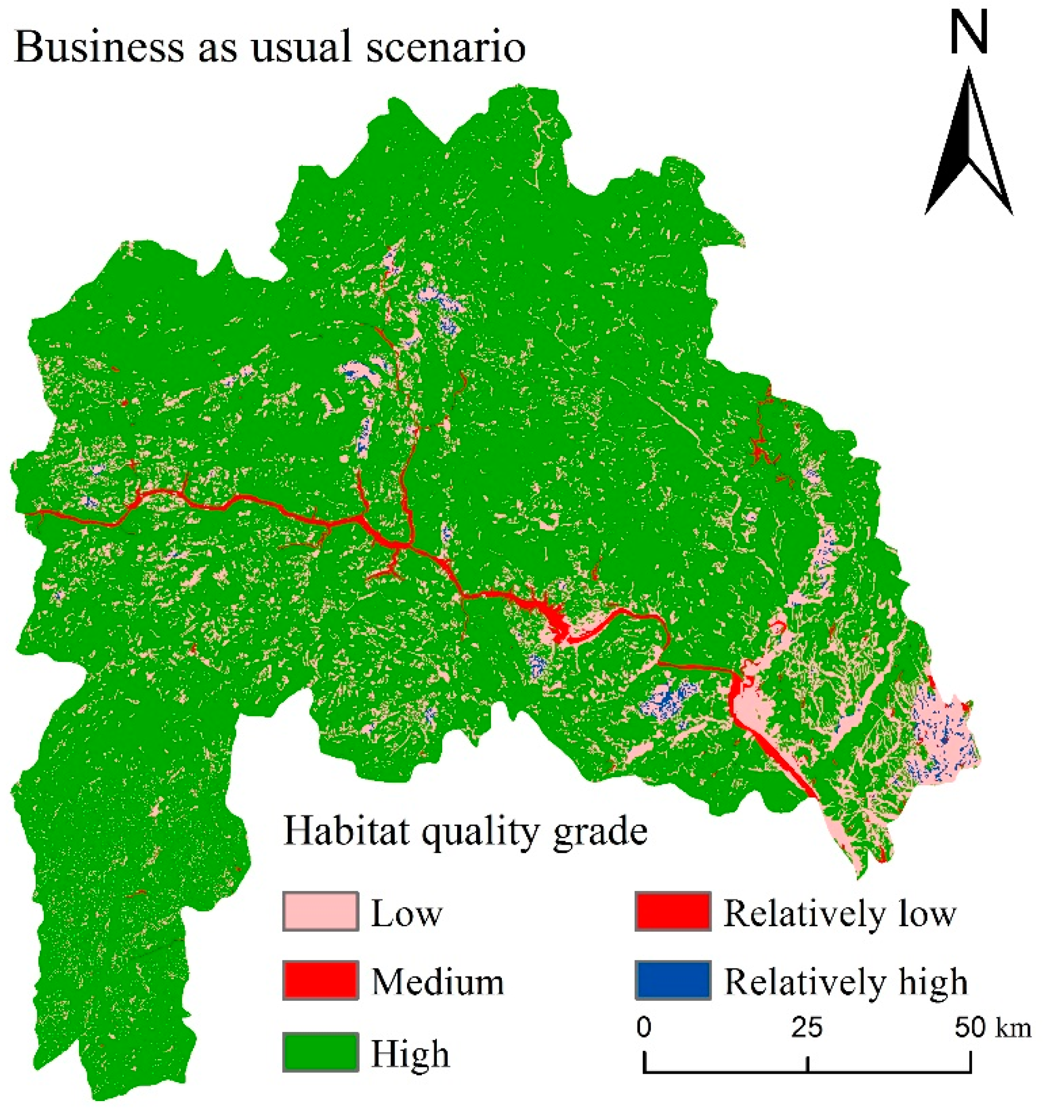
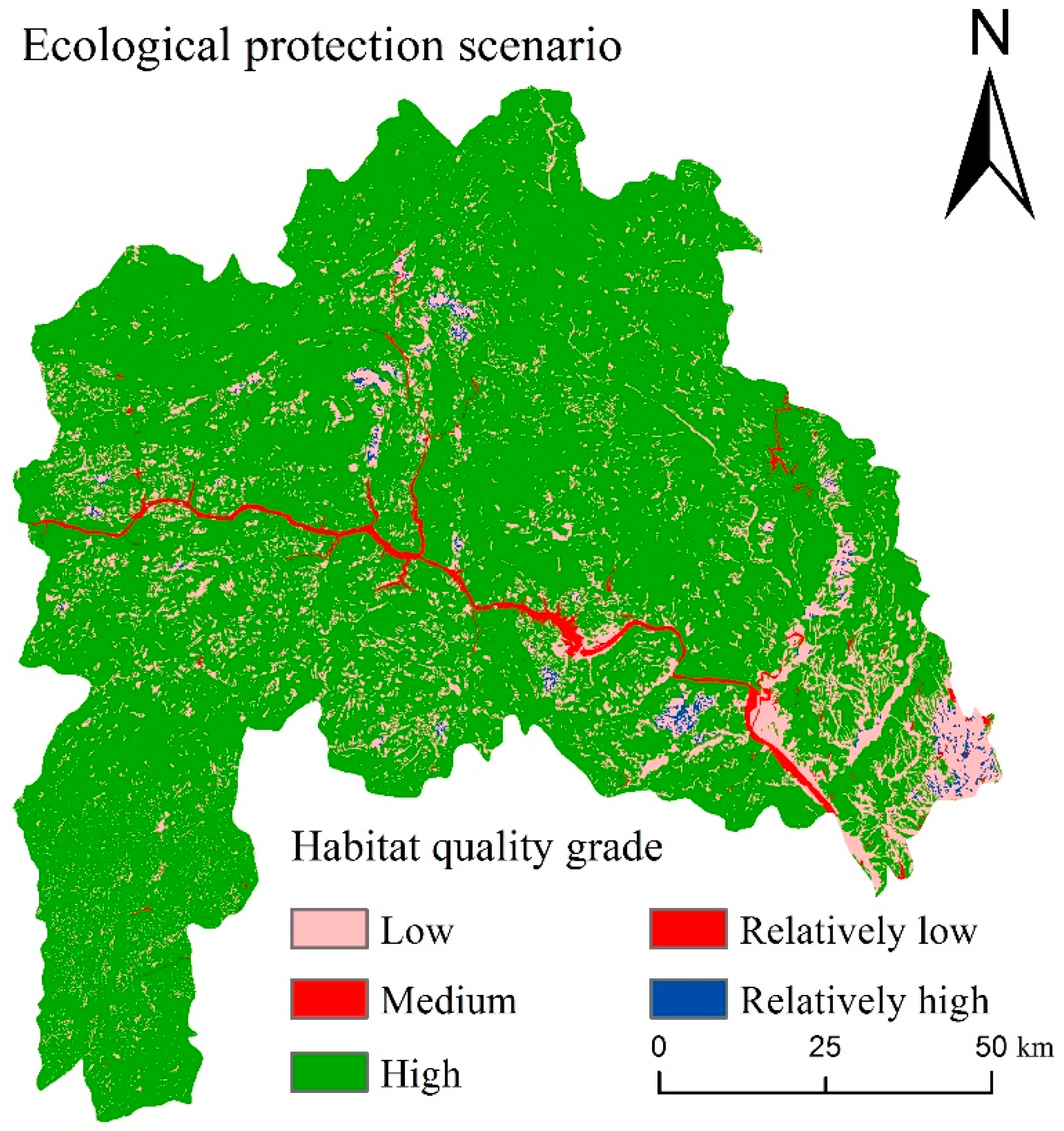
3.4.1. Forecast of Landscape Pattern
3.4.2. Prediction of Habitat Quality
4. Discussion
5. Conclusions
Author Contributions
Funding
Conflicts of Interest
References
- Daily, G.C.; Polasky, S.; Goldstein, J.; Kareiva, P.M.; Mooney, H.A. Ecosystem services in decision making: Time to deliver. Ecol. Environ. 2009, 7, 21–28. [Google Scholar] [CrossRef]
- Brath, A.; Montanari, A.; Moretti, G. Assessing the effect on flood frequency of land use change via hydrological simulation (with uncertainty). J. Hydrol. 2006, 324, 141–153. [Google Scholar] [CrossRef]
- Bormann, H.; Breuer, L.; Gräff, T.; Huisman, J.A. Analysing the effects of soil properties changes associated with land use changes on the simulated water balance: A comparison of three hydrological catchment models for scenario analysis. Ecol. Model. 2007, 209, 29–40. [Google Scholar] [CrossRef]
- Potschin, M.B.; Hainesyoung, R.H. Ecosystem services. Prog. Phys. Geogr. 2011, 35, 575–594. [Google Scholar] [CrossRef]
- Tallis, H.; Ricketts, T.; Nelson, E.; Ennaanay, D. InVEST 1.005 Beta Users Guide; The Natural Capital Project; Stanford University: Stanford, CA, USA, 2009. [Google Scholar]
- Hunsaker, C.T.; O’Neill, R.V.; Jackson, B.L.; Timmins, S.P.; Levine, D.A. Sampling to characterize landscape pattern. Landsc. Ecol. 1994, 9, 207–226. [Google Scholar] [CrossRef]
- Vitousek, P.M.; Mooney, H.A.; Lubchenco, J. Human domination of Earth’s ecosystems. Science 1997, 277, 494–499. [Google Scholar] [CrossRef]
- Wilcove, D.S.; Rothsetin, D.; Dubow, J.; Phillips, A.; Losos, E. Quantifying Threats to Imperiled Species in the United States Assessing the relative importance of habitat destruction, alien species, pollution, overeplotiation, and disease. Bioscience 1998, 48, 607–615. [Google Scholar] [CrossRef]
- Nüsser, M. Change and persistence: Contemporary landscape transformation in the Nanga Parbat region, northern Pakistan. Mt. Res. Dev. 2000, 20, 348–355. [Google Scholar] [CrossRef]
- Fairbanks, D.H.K.; Benn, G.A. Identifying regional landscapes for conservation planning: A case study from KwaZulu-Natal, South Africa. Landsc. Urban Plan. 2000, 50, 237–257. [Google Scholar] [CrossRef]
- Sitzia, T.; Semenzato, P.; Trentanovi, G. Natural reforestation is changing spatial patterns of rural mountain and hill landscapes: A global overview. For. Ecol. Manag. 2010, 259, 1354–1362. [Google Scholar] [CrossRef]
- López-Pujol, J.; Ren, M.X. Biodiversity and the Three Gorges Reservoir: A troubled marriage. J. Nat. Hist. 2009, 43, 2765–2786. [Google Scholar] [CrossRef]
- Wu, J.; Huang, J.; Han, X.; Xie, Z.; Gao, X.; Fangliang, H. Three-Gorges Dam–experiment in habitat fragmentation? Science 2003, 300, 1239–1240. [Google Scholar] [CrossRef] [PubMed]
- Wu, J.; Huang, J.; Han, X.; Gao, X.; He, F.; Jiang, M.; Jiang, Z.; Primack, R.B.; Shen, Z. The Three Gorges Dam: an ecological perspective. Ecol. Environ. 2004, 2, 241–248. [Google Scholar] [CrossRef]
- Kittinger, J.N.; Coontz, K.M.; Yuan, Z.; Han, D.; Zhao, X.; Wilcox, B.A. Toward holistic evaluation and assessment: Linking ecosystems and human well-being for the three gorges dam. EcoHealth 2009, 6, 601–613. [Google Scholar] [CrossRef] [PubMed]
- Scheller, R.M.; Domingo, J.B.; Sturtevant, B.R.; Williams, J.S.; Rudy, A. Design, development, and application of LANDIS-II, a spatial landscape simulation model with flexible temporal and spatial resolution. Ecol. Model. 2007, 201, 409–419. [Google Scholar] [CrossRef]
- Wang, X.; Yu, S.; Huang, G.H. Land allocation based on integrated GIS-optimization modeling at a watershed level. Landsc. Urban Plan. 2004, 66, 61–74. [Google Scholar] [CrossRef]
- Baldwin, D.J.B.; Weaver, K.; Schnekenburger, F.; Perera, H.A. Sensitivity of landscape pattern indices to input data characteristics on real landscapes: Implications for their use in natural disturbance emulation. Landsc. Ecol. 2004, 19, 255–271. [Google Scholar] [CrossRef]
- Agarwal, D.K.; Silander, J.A., Jr.; Gelfand, A.E.; Dewar, R.E. Tropical deforestation in Madagascar: Analysis using hierarchical, spatially explicit, Bayesian regression models. Ecol. Model. 2005, 185, 105–131. [Google Scholar] [CrossRef]
- Syphard, A.D.; Clarke, K.C.; Franklin, J. Using a cellular automaton model to forecast the effects of urban growth on habitat pattern in southern California. Ecol. Complex. 2005, 2, 185–203. [Google Scholar] [CrossRef]
- Bolliger, J.; Wagner, H.; Turner, M.G. Identifying and Quantifying Landscape Patterns in Space and Time; A Changing World; Springer: Dordrecht, The Netherlands, 2007; pp. 177–194. [Google Scholar]
- Fan, F.; Wang, Y.; Wang, Z. Temporal and spatial change detecting (1998–2003) and predicting of land use and land cover in Core corridor of Pearl River Delta (China) by using TM and ETM+ images. Environ. Monit. Assess. 2008, 137, 127–147. [Google Scholar] [CrossRef] [PubMed]
- Sang, L.; Zhang, C.; Yang, J.; Zhu, D.; Yun, W. Simulation of land use spatial pattern of towns and villages based on CA-Markov model. Math. Comput. Model. 2011, 54, 938–943. [Google Scholar] [CrossRef]
- Batty, M.; Xie, Y.; Sun, Z. Modeling urban dynamics through GIS-based cellular automata. Comput. Environ. Urban Syst. 1999, 23, 205–233. [Google Scholar] [CrossRef]
- Nourqolipour, R.; Shariff, A.R.B.M.; Balasundram, S.K.; Ahmad, N.B.; Sood, A.M. A GIS-based model to analyze the spatial and temporal development of oil palm land use in Kuala Langat district, Malaysia. Environ. Earth Sci. 2015, 73, 1687–1700. [Google Scholar] [CrossRef]
- Boumans, R.; Costanza, R. The multiscale integrated Earth Systems model (MIMES): The dynamics, modeling and valuation of ecosystem services. Glob. Water Syst. Res. 2008, 2, 1. [Google Scholar]
- Mohan, C.; Levine, F. ARIES/IM: An efficient and high concurrency index management method using write-ahead logging. ACM Sigmod Record 1992, 21, 371–380. [Google Scholar] [CrossRef]
- Wang, Y.; Bakker, F.; Groot, R.D.; Wörtche, H. Effect of ecosystem services provided by urban green infrastructure on indoor environment: A literature review. Build. Environ. 2014, 77, 88–100. [Google Scholar] [CrossRef]
- Natural Capital Project. Available online: https://naturalcapitalproject.stanford.edu (accessed on 14 May 2017).
- Haunreiter, E.; Cameron, D. Mapping Ecosystem Services in the Sierra Nevada, CA. Nat. Conserv. Calif. Program 2011, 12, 16–32. [Google Scholar]
- Mdk, L.; Matlock, M.D.; Cummings, E.C.; Nalley, L.L. Quantifying and mapping multiple ecosystem services change in West Africa. Agric. Ecosyst. Environ. 2013, 165, 6–18. [Google Scholar]
- Terrado, M.; Sabater, S.; Chaplin-Kramer, B.; Mandle, L.; Ziv, G. Model development for the assessment of terrestrial and aquatic habitat quality in conservation planning. Sci. Total. Environ. 2016, 540, 63–70. [Google Scholar] [CrossRef] [PubMed]
- Chen, K.Y. Ecosystem health: ecological sustainability target of strategic environment assessment. J. For. Res. 2003, 14, 146–150. [Google Scholar]
- Zhang, M.; Jin, H.; Cai, D.; Jiang, C. The comparative study on the ecological sensitivity analysis in Huixian karst wetland, China. Procedia Environ. Sci. 2010, 2, 386–398. [Google Scholar]
- United States Geological Survey (USGS). Available online: https://glovis.usgs.gov (accessed on 11 July 2017).
- United States Geological Survey (USGS). Global Data Explorer. Available online: https://gdex.cr.usgs.gov/gdex/ (accessed on 21 October 2017).
- Meteorological Data Sharing Service System of China. Available online: http://data.cma.cn/ (accessed on 30 December 2017).
- Elvidge, C.D. Mapping City Lights with Nighttime Data from the DMSP Operational Linescan System. Photogramm. Eng. Remote Sens. 1997, 63, 727–734. [Google Scholar]
- Zhao, G.; Dai, Z.; Hu, Y. The Suitability of Different Nighttime Light Data for GDP Estimation at Different Spatial Scales and Regional Levels. Sustainability 2017, 9, 305. [Google Scholar]
- National Oceanic and Atmospheric Administration (NOAA). Available online: https://www.ngdc.noaa.gov/eog/dmsp/downloadV4composites.html (accessed on 9 January 2018).
- Hulst, R.V. On the dynamics of vegetation: Markov chains as models of succession. Vegetation 1979, 40, 3–14. [Google Scholar] [CrossRef]
- Yang, X.; Zheng, X.Q.; Lv, L.N. A spatiotemporal model of land use change based on ant colony optimization, Markov chain and cellular automata. Ecol. Model. 2012, 233, 11–19. [Google Scholar] [CrossRef]
- Hou, W.; Walz, U. Enhanced analysis of landscape structure: Inclusion of transition zones and small-scale landscape elements. Ecol. Indic. 2013, 31, 15–24. [Google Scholar] [CrossRef]
- Ichikawa, K.; Okubo, N.; Okubo, S.; Takeuchi, K. Transition of the satoyama, landscape in the urban fringe of the Tokyo metropolitan area from 1880 to 2001. Landsc. Urban Plan. 2006, 78, 398–410. [Google Scholar] [CrossRef]
- Luo, G.; Amuti, T.; Zhu, L.; Mambetov, B.T.; Maisupova, B. Dynamics of landscape patterns in an inland river delta of Central Asia based on a cellular automata-Markov model. Reg. Environ. Chang. 2015, 15, 277–289. [Google Scholar] [CrossRef]
- Hu, X.L.; Xu, L.; Zhang, S.S. Land use pattern of Dalian City, Liaoning Province of Northeast China based on CA-Markov model and multi-objective optimization. Chin. J. Appl. Ecol. 2013, 24, 1652. [Google Scholar]
- Bayliss, J.L.; Simonite, V.; Thompson, S. The use of probabilistic habitat suitability models for biodiversity action planning. Agric. Ecosyst. Environ. 2005, 108, 228–250. [Google Scholar] [CrossRef]
- Holzkämper, A.; Lausch, A.; Seppelt, R. Optimizing landscape configuration to enhance habitat suitability for species with contrasting habitat requirements. Ecol. Model. 2006, 198, 277–292. [Google Scholar] [CrossRef]
- Seabrook, L.; Mcalpine, C.; Rhodes, J.; Baxter, G.; Bradley, A. Determining range edges: Habitat quality, climate or climate extremes? Divers. Distrib. 2014, 20, 95–106. [Google Scholar] [CrossRef]
- Almpanidou, V.; Mazaris, A.D.; Mertzanis, Y.; Avraam, I.; Antoniou, I. Providing insights on habitat connectivity for male brown bears: A combination of habitat suitability and landscape graph-based models. Ecol. Model. 2014, 286, 37–44. [Google Scholar] [CrossRef]
- Mckinney, M.L. Influence of settlement time, human population, park shape and age, visitation and roads on the number of alien plant species in protected areas in the USA. Divers. Distrib. 2002, 8, 311–318. [Google Scholar] [CrossRef]
- Forman, R.T.T.; Sperling, D.; Bissonette, J.A. Road Ecology: Science & Solutions. Landsc. Ecol. 2004, 19, 563–565. [Google Scholar]
- Forman, R.T.T. Some general principles of landscape and regional ecology. Landsc. Ecol. 1995, 10, 133–142. [Google Scholar] [CrossRef]
- Lindenmayer, D.; Cunningham, R.; Macgregor, C.; Crane, M.; Michael, D. Temporal Changes in Vertebrates during Landscape Transformation: A Large-Scale “Natural Experiment”. Ecol. Monogr. 2008, 78, 567–590. [Google Scholar] [CrossRef]
- Atkinson, P.M.; Massari, R. Generalized linear modeling of susceptibility to landsliding in the central Apennines, Italy. Comput. Geosci. 1998, 24, 373–385. [Google Scholar] [CrossRef]
- Pontius, R. Quantification Error versus Location Error in Comparison of Categorical Maps. Photogramm. Eng. Remote. Sens. 2000, 66, 1011–1016. [Google Scholar]
- Menard, S.W. Applied Logistic Regression Analysis (Quantitative Applications in the Social Sciences); SAGE Publications: Thousand Oaks, CA, USA, 2013. [Google Scholar]
- Lee, S. Application of logistic regression model and its validation for landslide susceptibility mapping using GIS and remote sensing data. Int. J. Remote Sens. 2005, 26, 1477–1491. [Google Scholar] [CrossRef]
- Ohlmacher, G.C.; Davis, J.C. Using multiple logistic regression and GIS technology to predict landslide hazard in northeast Kansas, USA. Eng. Geol. 2003, 69, 331–343. [Google Scholar] [CrossRef]
- Shu, B.; Zhang, H.; Li, Y.; Qu, Y.; Chen, L. Spatiotemporal variation analysis of driving forces of urban land spatial expansion using logistic regression: A case study of port towns in Taicang City, China. Habitat Int. 2014, 43, 181–190. [Google Scholar] [CrossRef]
- Hu, Z.; Lo, C.P. Modelling urban growth in Atlanta using logistic regression. Comput. Environ. Urban Syst. 2007, 31, 667–688. [Google Scholar] [CrossRef]
- Ozdemir, A. Using a binary logistic regression method and GIS for evaluating and mapping the groundwater spring potential in the Sultan Mountains (Aksehir, Turkey). J. Hydrol. 2011, 405, 123–136. [Google Scholar] [CrossRef]
- Ayalew, L.; Yamagishi, H. The application of GIS-based logistic regression for landslide susceptibility mapping in the Kakuda-Yahiko Mountains, Central Japan. Geomorphology 2005, 65, 15–31. [Google Scholar] [CrossRef]
- Dai, F.; Lee, C.F. Landslides on Natural Terrain: Physical Characteristics and Susceptibility Mapping in Hong Kong. Mt. Res. Dev. 2002, 22, 40–47. [Google Scholar] [CrossRef]
- Rgjr, P.; Schneider, L.C. Land-cover change model validation by a ROC method for the Ipswich watershed, Massachusetts, USA. Agric. Ecosyst. Environ. 2001, 85, 239–248. [Google Scholar]
- Guzzetti, F.; Cardinali, M.; Carrara, A.; Reichenbach, P. Use of GIS Technology in the Prediction and Monitoring of Landslide Hazard. Nat. Hazards 1999, 20, 117–135. [Google Scholar]
- Lee, S.; Min, K. Statistical analysis of landslide susceptibility at Yongin, Korea. Environ. Geol. 2001, 40, 1095–1113. [Google Scholar] [CrossRef]
- Dabbaghian, V.; Jackson, P.; Spicer, V.; Wuschke, K. A cellular automata model on residential migration in response to neighborhood social dynamics. Math. Comput. Model. 2010, 52, 1752–1762. [Google Scholar] [CrossRef]
- Morita, K.; Yamamoto, S. Effects of Habitat Fragmentation by Damming on the Persistence of Stream-Dwelling Charr Populations. Conserv. Boil. 2010, 16, 1318–1323. [Google Scholar] [CrossRef]
- Hall, C.J.; Jordaan, A.; Frisk, M.G. The historic influence of dams on diadromous fish habitat with a focus on river herring and hydrologic longitudinal connectivity. Landsc. Ecol. 2011, 26, 95–107. [Google Scholar] [CrossRef]
- Santuccijr, V.; Gephard, S.; Pescitelli, S. Effects of Multiple Low-Head Dams on Fish, Macroinvertebrates, Habitat, and Water Quality in the Fox River, Illinois. N. Am. J. Fish. Manag. 2005, 25, 975–992. [Google Scholar] [CrossRef]
- Harper, J.L.; Hawksworth, D.L. Biodiversity: Measurement and estimation. Philos. Trans. R. Soc. Lond. 1994, 345, 5. [Google Scholar] [CrossRef] [PubMed]
- Rey-Benayas, J.M.; Pope, K.O. Landscape Ecology and Diversity Patterns in the Seasonal Tropics from Landsat TM Imagery. Ecol. Appl. 1995, 5, 386–394. [Google Scholar] [CrossRef]
- Jabbar, M.T.; Shi, Z.H.; Wang, T.W.; Cai, C.F. Vegetation Change Prediction with Geo-Information Techniques in the Three Gorges Area of China. Pedosphere 2006, 16, 457–467. [Google Scholar] [CrossRef]
- Mcneely, J.A. Expanding Partnerships in Conservation; Island Press: Washington, DC, USA, 1995. [Google Scholar]
- Chape, S.; Harrison, J.M.; Lysenko, I. Measuring the extent and effectiveness of protected areas as an indicator for meeting global biodiversity targets. Philos. Trans. Boil. Sci. 2005, 360, 443–455. [Google Scholar] [CrossRef] [PubMed]
- Hockings, M.; Stolton, S.; Leverington, F.; Dudley, N.; Courrau, J. Assessing Effectiveness—A Framework for Assessing Management Effectiveness of Protected Areas. Arch. Pediatr. Urug. 2007, 71, 5–9. [Google Scholar]
- Lu, Q.; Ning, J.; Liang, F.; Bi, X. Evaluating the Effects of Government Policy and Drought from 1984 to 2009 on Rangeland in the Three Rivers Source Region of the Qinghai-Tibet Plateau. Sustainability 2017, 9, 1033. [Google Scholar] [CrossRef]
- Nagendra, H. Drivers of regrowth in South Asia’s human impacted forests. Curr. Sci. 2009, 97, 1586–1592. [Google Scholar]
- Adhikari, S.; Southworth, J. Simulating Forest Cover Changes of Bannerghatta National Park Based on a CA-Markov Model: A Remote Sensing Approach. Remote Sens. 2012, 4, 3215–3243. [Google Scholar] [CrossRef]
- Sharma, R.; Nehren, U.M.; Rahman, S.A.; Meyer, M.; Baral, H. Modeling Land Use and Land Cover Changes and Their Effects on Biodiversity in Central Kalimantan, Indonesia. Land 2018, 7, 57. [Google Scholar] [CrossRef]
- Nelson, E.; Mendoza, G.; Regetz, J.; Polasky, S.; Tallis, H. Modeling multiple ecosystem services, biodiversity conservation, commodity production, and tradeoffs at landscape scales. Front. Ecol. Environ. 2009, 7, 4–11. [Google Scholar] [CrossRef]
- Nelson, E.J.; Daily, G.C. Modelling ecosystem services in terrestrial systems. F1000 Biol. Rep. 2010, 2, 53. [Google Scholar] [CrossRef] [PubMed]


| First Class | Second Class | First Class | Second Class |
|---|---|---|---|
| Farmland | Paddy field | Grassland | High coverage grassland |
| Dry land | Moderate coverage grassland | ||
| Woodland | Thick woodland | Low coverage grassland | |
| Shrubbery land | Construction land | Urban land | |
| Sparse woodland | Rural residential land | ||
| Other woodland | Industrial and traffic land | ||
| Waters | Canal | Unused land | Dene |
| Lake | Gobi | ||
| Reservoir or pond | Saline and alkaline land | ||
| Permanent ice and snow | Marshland | ||
| Tideland | Bare land | ||
| Shoaly land | Bare rock | ||
| Other |
| Landscape Types | Habitat | Paddy Fields | Dry Land | Urban Land | Rural Resident Land | Industrial and Traffic Land | Bare Land |
|---|---|---|---|---|---|---|---|
| Paddy field | 0 | 0 | 1 | 0 | 0 | 0.5 | 0.4 |
| Dry land | 0 | 1 | 0 | 0 | 0 | 0.5 | 0.4 |
| Thick woodland | 1 | 1 | 1 | 0.2 | 0.2 | 0.3 | 0.3 |
| Shrubbery land | 1 | 0.5 | 0.5 | 0.2 | 0.2 | 0.2 | 0.1 |
| Sparse woodland | 1 | 0.7 | 0.9 | 0.2 | 0.8 | 0.4 | 0.8 |
| Other woodland | 1 | 0.5 | 0.5 | 0.2 | 0.2 | 0 | 0 |
| High coverage grassland | 0.5 | 0.8 | 0.8 | 0.4 | 0.7 | 0.4 | 0.4 |
| Moderate coverage grassland | 1 | 0.5 | 0.5 | 0.2 | 0.2 | 0 | 0 |
| Low coverage grassland | 1 | 0.8 | 0.8 | 0 | 0 | 0.4 | 0.4 |
| Canal | 0 | 0.3 | 0.3 | 0.3 | 0.3 | 0.8 | 0.2 |
| Lake | 1 | 0.5 | 0.4 | 0 | 0 | 0.4 | 0.4 |
| Reservoir or pond | 1 | 0 | 1 | 0.7 | 0.4 | 0.4 | 0.6 |
| Shoaly land | 1 | 0.8 | 0.8 | 0 | 0 | 0.4 | 0.4 |
| Urban land | 0 | 0 | 0 | 0 | 0 | 0.8 | 0.7 |
| Rural residential land | 0.6 | 0.2 | 0.2 | 0 | 0 | 0 | 0.8 |
| Industrial and traffic land | 0.7 | 0.2 | 0.2 | 0 | 0 | 0 | 0.8 |
| Bare land | 0.5 | 0.2 | 0.2 | 0 | 0 | 0 | 0.8 |
| Threat | Maximum Effective Distance (km) | Weight | DECAY |
|---|---|---|---|
| Paddy fields | 0.5 | 0.5 | Exponential |
| Dry land | 0.5 | 0.5 | Exponential |
| Urban land | 3 | 0.7 | Exponential |
| Rural residential land | 2 | 0.7 | Exponential |
| Industrial and traffic land | 8 | 1 | Linear |
| Bare land | 10 | 0.3 | Exponential |
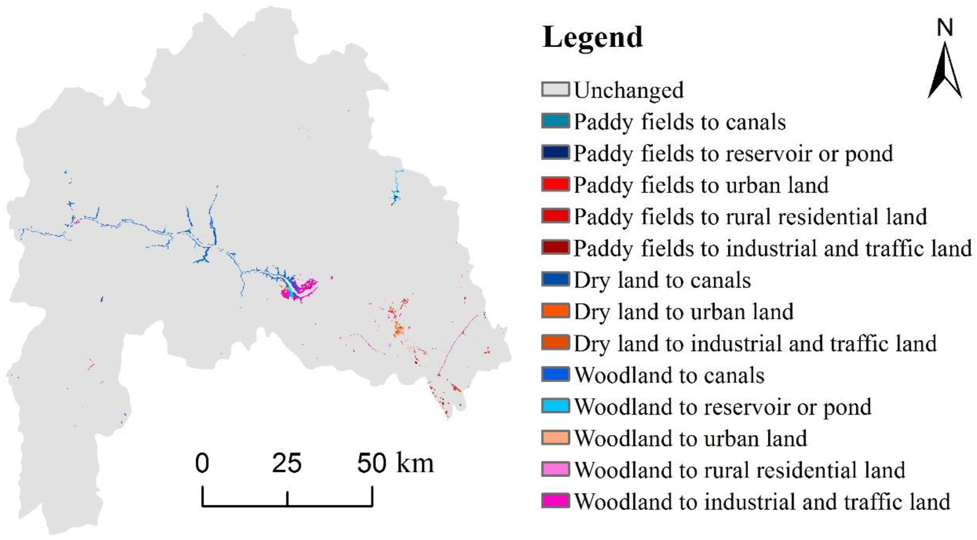
| Changed Type | Area | Percentage |
|---|---|---|
| Unchanged | 12,067.19 | 98.62 |
| Woodland to canals | 41.52 | 0.34 |
| Woodland to industrial and traffic land | 26.21 | 0.22 |
| Woodland to reservoir or pond | 8.23 | 0.07 |
| Woodland to urban land | 6.84 | 0.06 |
| Paddy fields to canal | 3.82 | 0.03 |
| Paddy field to industrial and traffic land | 3.77 | 0.03 |
| Paddy fields to urban land | 3.43 | 0.03 |
| Dry land to urban land | 3.31 | 0.03 |
| Dry land to industrial and traffic land | 3.28 | 0.03 |
| Dry land to canals | 2.95 | 0.02 |
| Woodland to rural residential land | 2.90 | 0.02 |
| Paddy fields to reservoir or pond | 2.51 | 0.02 |
| Paddy fields to rural residential land | 2.32 | 0.02 |
| Grade | Value Range | Description |
|---|---|---|
| Low | 0~0.1 | Poor habitat quality |
| Relatively low | 0.1~0.6 | Relatively poor habitat quality |
| Medium | 0.6~0.8 | Medium habitat quality |
| Relatively high | 0.8~0.9 | Relatively high habitat quality |
| High | 0.9~1 | High habitat quality |
| Grade | 1990 | 2000 | 2010 | 1990 to 2010 | ||||
|---|---|---|---|---|---|---|---|---|
| Area | Percentage | Area | Percentage | Area | Percentage | Area | Percentage | |
| Low | 1664.66 | 13.60 | 1707.71 | 13.95 | 1701.48 | 13.90 | 36.81 | 0.30 |
| Relatively low | 100.28 | 0.82 | 99.53 | 0.81 | 153.90 | 1.26 | 53.62 | 0.44 |
| Medium | 30.18 | 0.25 | 32.14 | 0.26 | 36.27 | 0.30 | 6.08 | 0.05 |
| Relatively high | 68.45 | 0.56 | 67.83 | 0.55 | 65.39 | 0.53 | −3.06 | −0.03 |
| High | 10,379.36 | 84.78 | 10,337.74 | 84.42 | 10,287.91 | 84.02 | −91.45 | −0.76 |
| Independent Parameter | Paddy Field | Dry Land | Woodland | Grassland | Canal | Lake | Reservoir or Pond | Shoaly Land | Urban Land | Rural Residential Land | Industrial and Traffic Land | Bare Land |
|---|---|---|---|---|---|---|---|---|---|---|---|---|
| Intercept | −4.30 | −2.62 | −2.34 | −0.11 | 17.70 | −161.50 | 1.29 | −18.74 | −378.72 | −37.42 | −28.93 | −1136.34 |
| X1 | −0.79 | 0.44 | 0.40 | 84.61 | 543.06 | 2.21 | −0.64 | 2.15 | 7.13 | 827.33 | 0.00 | 392.10 |
| X2 | −0.49 | −0.40 | −0.84 | −0.38 | −0.05 | 6.94 | 1.23 | −0.38 | −1.35 | 1.52 | −2.09 | 4.08 |
| X3 | −58.21 | −4.04 | −32.79 | 4.45 | −369 | −368.32 | 102.37 | 202.56 | 124.07 | 9.55 | −74.06 | 478.59 |
| X4 | 71.12 | 7.93 | 48.93 | 3.81 | 428.69 | 480.34 | −130.03 | −193.84 | −11.88 | 316.47 | 71.66 | −705.36 |
| X5 | 2.60 | 1.08 | −5.16 | −10.89 | −17.26 | −74.72 | 23.38 | −8.73 | −23.62 | −9.02 | 21.00 | −24.43 |
| X6 | 1.80 | −13.27 | −12.43 | −40.05 | −300 | 1757.60 | 87.07 | −161.30 | −1079.92 | 483.07 | 298.85 | 16,293.71 |
| X7 | −1.70 | 16.32 | 15.94 | 48.65 | 363.17 | −2082 | −87.57 | 159.51 | 467,520 | −587.76 | −362.09 | −19725 |
| X8 | 0.10 | 0.03 | −0.08 | 0.00 | −0.73 | 7.65 | −0.59 | −0.15 | −1.05 | 0.81 | 0.33 | −5.64 |
| X9 | 0.00 | −0.01 | 0.04 | −0.02 | 0.13 | 0.00 | −0.12 | 0.10 | −0.06 | 0.37 | 0.02 | −12.95 |
| X10 | 0.07 | 0.02 | 0.07 | 0.13 | 0.35 | −1.82 | 0.06 | −0.02 | −1.04 | −0.39 | −0.79 | −9.33 |
| X11 | 0.04 | 0.02 | 0.12 | 0.00 | 0.30 | 0.05 | 0.11 | 0.06 | −0.10 | 0.36 | 0.34 | 12.06 |
| X12 | 0.01 | 0.02 | −0.12 | −0.03 | 0.33 | 4.41 | 0.20 | −0.44 | 2.00 | 1.07 | −0.25 | 43.52 |
| X13 | −0.44 | −0.18 | −0.37 | −0.39 | 0.35 | 8.53 | −0.44 | 0.02 | 0.28 | 1.21 | −2.23 | 23.70 |
| X14 | −0.07 | −0.07 | −0.14 | −0.08 | −0.51 | −7.18 | 0.22 | 0.03 | −192.14 | −0.97 | −0.08 | −105.56 |
| X15 | 0.21 | −0.06 | 0.04 | −0.12 | 0.53 | −2.62 | 0.55 | 0.06 | −1.40 | −349.51 | 0.33 | 9.22 |
| ROC | 0.94 | 0.83 | 0.92 | 0.86 | 0.99 | 0.85 | 0.95 | 0.98 | 0.90 | 0.88 | 0.98 | 0.87 |
| Habitat Quality Grade | 2010 | 2020 | 2010 to 2020 | |||
|---|---|---|---|---|---|---|
| Area | Percentage | Area | Percentage | Area | Percentage | |
| Low | 1701.48 | 13.90 | 1721.38 | 14.06 | 19.90 | 0.16 |
| Relatively low | 153.90 | 1.26 | 152.28 | 1.24 | −1.62 | −0.02 |
| Medium | 36.27 | 0.30 | 33.57 | 0.28 | −2.70 | −0.02 |
| Relatively high | 65.39 | 0.53 | 59.99 | 0.49 | −5.40 | −0.04 |
| High | 10,287.91 | 84.02 | 10,274.39 | 83.92 | −13.52 | −0.10 |
| Habitat Quality Grade | 2010 | 2020 | 2010 to 2020 | |||
|---|---|---|---|---|---|---|
| Area | Percentage | Area | Percentage | Area | Percentage | |
| Low | 1701.48 | 13.90 | 1681.52 | 13.73 | −19.96 | −0.17 |
| Relatively low | 153.90 | 1.26 | 148.34 | 1.21 | −5.57 | −0.05 |
| Medium | 36.27 | 0.30 | 31.59 | 0.26 | −4.68 | −0.04 |
| Relatively high | 65.39 | 0.53 | 72.78 | 0.61 | 7.39 | 0.08 |
| High | 10,287.91 | 84.02 | 10,301.95 | 84.14 | 14.04 | 0.12 |
© 2018 by the authors. Licensee MDPI, Basel, Switzerland. This article is an open access article distributed under the terms and conditions of the Creative Commons Attribution (CC BY) license (http://creativecommons.org/licenses/by/4.0/).
Share and Cite
Chu, L.; Sun, T.; Wang, T.; Li, Z.; Cai, C. Evolution and Prediction of Landscape Pattern and Habitat Quality Based on CA-Markov and InVEST Model in Hubei Section of Three Gorges Reservoir Area (TGRA). Sustainability 2018, 10, 3854. https://doi.org/10.3390/su10113854
Chu L, Sun T, Wang T, Li Z, Cai C. Evolution and Prediction of Landscape Pattern and Habitat Quality Based on CA-Markov and InVEST Model in Hubei Section of Three Gorges Reservoir Area (TGRA). Sustainability. 2018; 10(11):3854. https://doi.org/10.3390/su10113854
Chicago/Turabian StyleChu, Lin, Tiancheng Sun, Tianwei Wang, Zhaoxia Li, and Chongfa Cai. 2018. "Evolution and Prediction of Landscape Pattern and Habitat Quality Based on CA-Markov and InVEST Model in Hubei Section of Three Gorges Reservoir Area (TGRA)" Sustainability 10, no. 11: 3854. https://doi.org/10.3390/su10113854
APA StyleChu, L., Sun, T., Wang, T., Li, Z., & Cai, C. (2018). Evolution and Prediction of Landscape Pattern and Habitat Quality Based on CA-Markov and InVEST Model in Hubei Section of Three Gorges Reservoir Area (TGRA). Sustainability, 10(11), 3854. https://doi.org/10.3390/su10113854