An Entropy Approach to Regional Differences in Carbon Dioxide Emissions: Implications for Ethanol Usage

Abstract

The growth of the U.S. economy has been accompanied with a significant rise in carbon dioxide (CO₂) emissions. As CO₂ emissions are dependent on regional climatic conditions and energy-related activities in states, this study examines the extent to which the distribution of CO₂ emissions vary across nine climatically consistent regions in the U.S. The results obtained from the entropy approach reveal that the inequalities of CO₂ emissions vary across the regions. While the total inequality of CO₂ emissions is determined by the between-region and the average within-region inequalities, the between-region inequality begins to dominate the average within-region inequalities around 1980s; the emission inequalities between regions increase, but those within each region decrease. Given that ethanol usage is relevant to energy-related CO₂ emissions, this study also evaluates the impact of ethanol usage on the changes in the emission inequalities. The results show that an increase in the ratio of ethanol to fossil fuels is associated closely with the reductions in the inequalities of CO₂ emissions.

1. Introduction

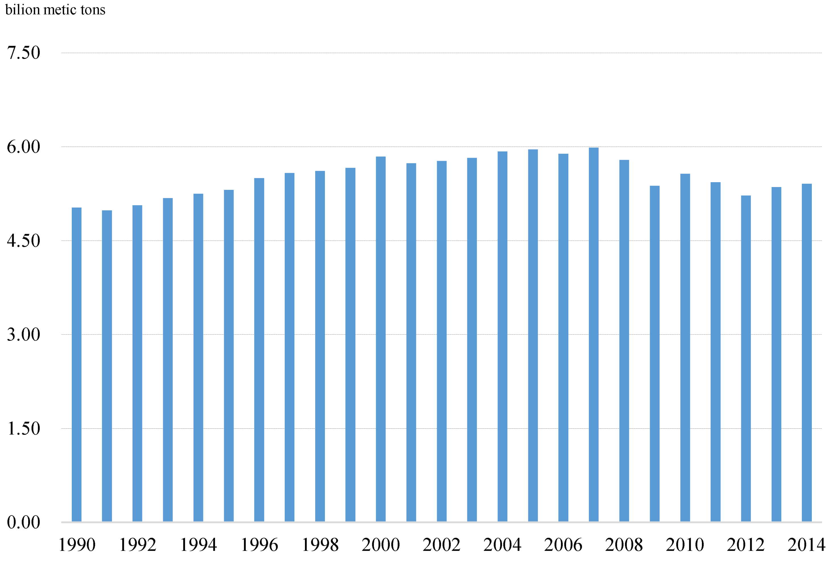
Carbon dioxide (CO₂) emissions are of great concerns because the emissions are considered as the primary source of greenhouse gases causing climate change and global warming; CO₂ emissions account for about 82% of all greenhouse gas emissions. According to the U.S. Environmental Protection Agency (EPA), in 2014, about 5.5 billion metric tons of CO₂ were released into the atmosphere; the U.S. was ranked the second in the world after China. Specifically, the emissions from the electricity, transportation, industry, residential and commercial usage, and non-fossil fuel combustion accounted for about 35%, 32%, 15%, 10%, and 7%, respectively. The main sources of CO₂ emissions were attributed to human activities burning fossil fuels for energy, transportation, and industrial uses. As the U.S. economy has grown with a substantial combustion of fossil fuels, the amount of CO₂ has also steadily increased by about 6% between 1990 and 2015 (Figure 1).

A vast literature has focused on the relationship between economic growth and environmental quality. The hypothesis of the Environmental Kuznets Curve (EKC), for example, conjectured that environmental quality would tend to improve due to the increasing demand for high quality of environment if an economy achieved a certain level of income [1,2]. Several studies tested for the EKC hypothesis to understand the linkage between income growth and CO₂ emissions, but they provided mixed empirical results [3,4,5,6,7,8,9,10]. In addition, the research was extended to examine the convergence of per capita CO₂ emissions across regions [11,12,13,14] and investigate the energy-related CO₂ emissions associated with changes in population growth, economic circumstance, and technological improvement [15,16,17,18,19].

While a growth of an economy is relevant to an increase in CO₂ emissions, the U.S. has pursued to reduce the energy-related CO₂ emissions with a variety of policy measures. According to the EPA, the U.S. facilitated to develop fuel-efficient vehicles and devices. Improving energy efficiency in fossil-fuel dependent vehicles and devices would reduce the use of fossil fuels, and in turn, CO₂ emissions. Along with the improvement of energy efficiency, the U.S. also encouraged energy conservation through education and training about energy-saving techniques. Many educational programs would help end-users reduce the use of fossil fuels and invest in energy-saving equipment. In addition, the U.S. considered carbon dioxide capture and sequestration as a strategy for preventing CO₂ emissions from entering the atmosphere. Furthermore, it pursued the conversion of fossil fuels to renewable fuels. Particularly, the use of corn-based ethanol was encouraged by the U.S. government since the abundance of corn in the U.S. made it feasible to switch the use of carbon energy (i.e., fossil fuels) to non-carbon energy (i.e., ethanol).

Among the policy measures reducing energy-related CO₂ emissions, the ethanol policy was paid extensive attention in the U.S. Considering the contribution of ethanol to energy security and environmental sustainability, the U.S. offered federal tax credits to subsidize those who blended ethanol with gasoline under the Energy Tax Act of 1978. Afterwards, the U.S. changed the subsidy policy to require the mandatory usage of ethanol under the Energy Policy Act of 2005 [20]. The Renewable Fuel Standard (RFS) program was established to facilitate a substantial growth in the ethanol market through the ethanol mandate. Moreover, the Energy Independence and Security Act of 2007 expanded the mandate to cover renewable fuel, advanced biofuel, cellulosic biofuel, and biomass-based diesel. Due to the governmental support, ethanol production increased dramatically from 83 million gallons to 15 billion gallons between 1981 and 2016, which amounted to over 90% of domestic ethanol consumption [21].

According to the EPA, CO₂ emissions vary with energy sources as well as climatic conditions. While different climatic conditions require different energy usage, the extent to which energy affects the amount of CO₂ varies with the properties of energy sources. The EPA defines the CO₂ emission coefficients as an indicator of measuring how much fuel combustion generates CO₂. For instance, the coefficients for ethanol, biodiesel and petroleum are, on average, 0.068, 0.071 and 0.073, respectively, which represents metric tons of CO₂ per million Btu. of each energy source. The use of ethanol generates low CO₂ emissions relative to other energy sources. As ethanol is a renewable energy source that reduces the amount of carbon emitted from ethanol combustion, the gasoline-ethanol blend can contribute to a reduction in CO₂ emissions. Moreover, CO₂ emissions released from the use of ethanol can be recaptured as corn is grown subsequently [22,23,24].

Given that CO₂ emissions are related closely with energy usage [25,26,27], the objectives of this study are two-fold. First, this study aims to investigate the extent to which regional disparities of CO₂ emissions exist in the U.S. Since energy usage is relevant to climatic conditions, this study reflects the regional similarities of climatic conditions to measure regional CO₂ emissions. This study uses the categorization of nine climatically consistent regions within the contiguous U.S. defined by the National Centers for Environmental Information. The Theil’s index is used to identify the regional inequalities of CO₂ emissions with respect to a growth in population. Second, this study tests whether the use of ethanol contributes to the emission inequalities across the regions. If ethanol substitutes for fossil fuels, thereby generating less CO₂ emissions, the emission inequalities may decrease as ethanol becomes an increasing portion of total energy use.

The findings will contribute to sustainable transformation into green economy. Measuring how CO₂ emissions vary regionally with population over time will be critical information for formulating carbon-related environmental policies. As the sustainable transformation occurs unevenly across regions, the information about regional discrepancy of CO₂ emissions is needed for understanding CO₂ emissions under different climatic conditions. In addition, the emissions are relevant to energy sources. Relatively less concentrated CO₂ emissions induced by using ethanol may contribute to providing local and national policy makers with crucial information about ethanol policies. The findings will be also useful for stakeholders involved in the ethanol industry because the governmental decisions will affect the sustainable growth of the industry. If replacing fossil fuels with ethanol contributes to reducing the regional inequality of CO₂ emissions, ethanol usage may be a viable way of achieving energy security and environmental improvement in the context of sustainable development.

2. Methodology

According to information theory, entropy quantifies the amount of information contained in random variables [28]. The entropy $\left(J\right)$ is measured by $J=-{\sum }_{i=1}^N{q}_i\ln \left(q_i\right)$ where $q_i$ is a probability that an event occurs for $i=1,\cdots ,N$, which is generally regarded as an information measure of uncertainty inherent in the variable. Kullback and Leibler [29] measured the differences in information between two probability distributions, and Theil [30] developed the inequality measure to capture the extent to which the distributions of variables differ from each other. Specifically, the Theil index measures the discrepancy between distributions of random variables to show the information inequality between the prior distribution and the posterior distribution [29,30]. Given the probability of each outcome, the prior probability and the posterior probability indicate the probability before and after information is received, respectively. Since a large divergence between two distributions implies that the prior is uninformative for the posterior, the Theil index represents whether the prior distribution has enough information to predict the posterior distribution [31].

Following Salois [32], we define the cross-entropy $\left(I_t\right)$ at time t as the information inequality between two probability distributions, which is expressed as

$$I_t={\sum }_{i=1}^N{y}_{it}\ln \left(\frac{y_{it}}{x_{it}}\right)$$

(1)

where $x_{it}$ and $y_{it}$ are the $i$th individual’s prior and posterior probabilities at time $t$ for $i=1,\cdots ,N$ and $t=1,\cdots ,T$, respectively. As $x_{it}$ and $y_{it}$ are probabilities that are non-negative and sum to unity, the probabilities of random variables are replaced with the shares of the variables because the shares also satisfy the properties of probabilities. In the field of economics, the entropy can be defined in terms of the shares of economic variables to examine the inequalities of their distributions [31,32,33,34,35,36,37,38,39,40].

In this study, the cross-entropy is used to examine the inequality in the regional distributions of CO₂ emissions in relation to population in the United States. When $c_{it}$ is the CO₂ emission share of state $i$ in a particular region at time $t$, the emission share is expressed as

$$c_t=\frac{C_{it}}{{\sum }_{i=1}^N{C}_{it}}$$

(2)

where $C_{it}$ is the emission level released from state $i$ at time $t$, and ${\sum }_{i=1}^N{C}_{it}$ is the total level of emissions released from all states at time $t$. Similarly, let $p_t$ be the population share of state $i$ in a particular region at time $t$. The population share is written as

$$p_t=\frac{P_{it}}{{\sum }_{i=1}^N{P}_{it}}$$

(3)

where $P_{it}$ is the population level of state $i$ at time $t$, and ${\sum }_{i=1}^N{P}_{it}$ is the total population level of all states at time $t$.

The cross-entropy index is now defined as

$$E_t={\sum }_{i=1}^N{c}_{it}\ln \left(\frac{c_{it}}{p_{it}}\right)$$

(4)

which is interpreted as a measure of emission-inequality. The emission-inequality measure $\left(E_t\right)$ approaches to zero as the differences in the per-capita emissions among states decline, but it approaches to infinity as the differences rise. Since this informational approach assumes that a distributional change sends a signal to another distributional change, the emission-inequality measure converges to zero as the population share contains information enough to predict the emission share.

The cross-entropy measure can be used to calculate the total entropy using the between-region entropy and the within-region entropy. Suppose that a region involves several states that have similar weather conditions. When the states are located in region $r$ for $=1,\cdots ,T$ $\left(R\le N\right)$, the between-region $\left(B_t\right)$ and within-region $\left(W_t\right)$ entropies are calculated by

$$\begin{gathered} B_t={\sum }_{r=1}^R{C}_{rt}\ln \left(\frac{C_{rt}}{P_{rt}}\right) \\ {W}_t=\sum _{i=1}^r\frac{c_{it}}{C_{rt}}\ln \left(\frac{\frac{c_{it}}{C_{rt}}}{\frac{p_{it}}{P_{rt}}}\right) \end{gathered}$$

(5)

where the emission share of region $r$ is defined as $C_{rt}={\sum }_{i=1}^r{c}_{it}$, and the population share of region $r$ is defined as $P_{rt}={\sum }_{i=1}^r{p}_{it}$.

The aggregate or total entropy $\left(A_t\right)$ is the sum of the between-region entropy and the average within-region entropy, which is

$$A_t=B_t+{\sum }_{r=1}^R{C}_{rt}{W}_t$$

(6)

where the average within-region entropy is the weighted sum of the within-region entropies. The between-region entropy measures the inequality between the $R$ regions, while the within-region entropy measures the inequality across states in region $r$.

Based on the entropies, we test whether the regional differences in CO₂ emissions are associated with the replacement of fossil fuels with ethanol. Following the approach of Mishra et al. [33], we construct an econometric model as

$$Y_t={\alpha }_0+{\alpha }_1{X}_t+{\alpha }_2{T}_t+{\epsilon }_t$$

(7)

where $Y_t$ can indicate the average within-region entropy, the between-region entropy, or the aggregate (total) entropy. In this specification, $X_t$ is the amount of ethanol relative to the amount of fossil fuels, which represents the extent to which ethanol substitutes for fossil fuels. In addition, $T_t$ is the time trend, and ${\epsilon }_t$ is the error term with the normal distribution. This model is estimated by the generalized least squares with the bootstrapping method to account for heteroskedasticity and normality of the error term. The estimation tests mainly for the hypothesis that the use of ethanol affects the regional disparities of CO₂ emissions.

3. Data and Results

The National Centers for Environmental Information have identified nine climatically consistent regions within the contiguous United States.

Table 1. The U.S. Climate Regions.

Regions	States
Central	Illinois, Indiana, Kentucky, Missouri, Ohio, Tennessee, West Virginia
East North Central	Iowa, Michigan, Minnesota, Wisconsin
Northeast	Connecticut, Delaware, Maine, Maryland, Massachusetts, New Hampshire, New Jersey, New York, Pennsylvania, Rhode Island, Vermont
Northwest	Idaho, Oregon, Washington
South	Arkansas, Kansas, Louisiana, Mississippi, Oklahoma, Texas
Southeast	Alabama, Florida, Georgia, North Carolina, South Carolina, Virginia
Southwest	Arizona, Colorado, New Mexico, Utah
West	California, Nevada
West North Central	Montana, Nebraska, North Dakota, South Dakota, Wyoming

Source: The National Centers for Environmental Information.

shows the U.S. climate regions that consist of nine regions covering 48 U.S. states, which is useful for understanding current climate anomalies between regions [41]. This study uses this categorization to identify the regional changes in CO₂ emissions, which reflects population segment under similar climatic conditions.

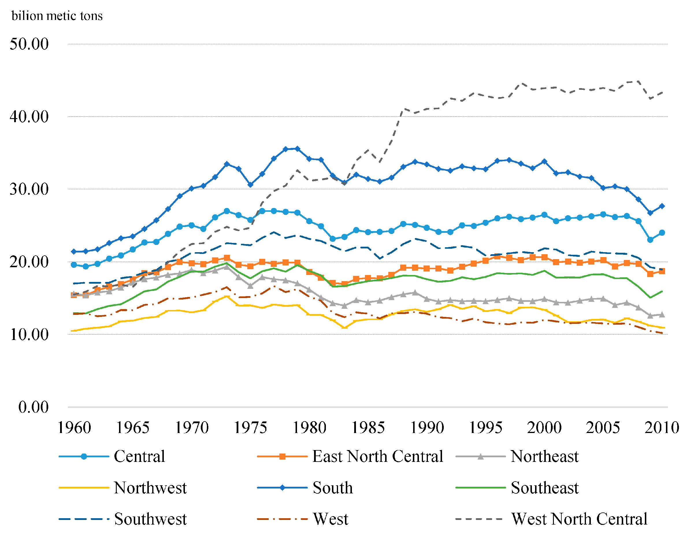
Based on the categorization of regions, the per-capita emissions are compared across the regions. Figure 2 shows that the per-capita emissions have continued to increase with similar patterns in most regions. The average per-capita emission level was 15.6 billion metric tons, but it increased to 20.3 billion metric tons. In particular, the per-capita CO₂ emissions began to increase after 1980s at decreasing rates in most regions. The northwest region has the lowest emission level over the period, whereas the central and west north central regions have higher emission levels than other regions. While the central region’s emission level began to decline, hitting 27.0 billion metric tons in 1977, the west north central region’s emission level increased from 15.5 to 43.4 billion metric tons. The changes in the per-capita emissions became stable after 1980 in most regions, but the west north central region experienced an exceptional increase in per-capital emissions. The changes in the per-capita emissions may be attributable to different human activities relevant to the transformation into different energy sources.

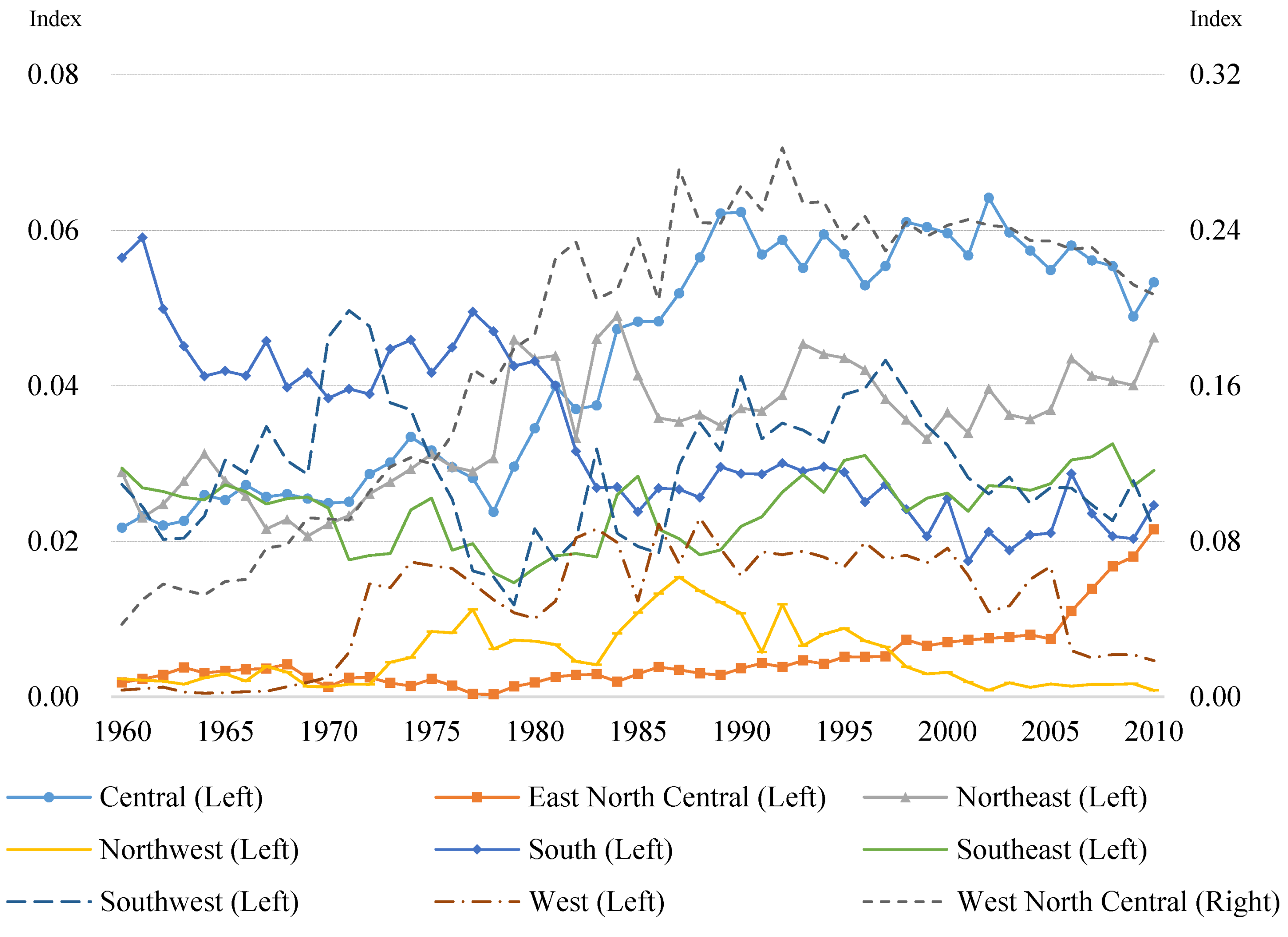
Figure 3 presents the nine within-region inequalities of CO₂ emissions calculated by Equation (4). The higher value is, the greater inequality of CO₂ emissions exists between states within a region. Most within-region inequalities of CO₂ emissions range from 0 to 0.28, which implies that the population growth in each region signals similar information about CO₂ emissions. Specifically, the east north central, northwest, west regions have lowest inequality with less fluctuations; the northwest region has the lowest dispersion of CO₂ emissions across states within the region. These regions reveal that there is little difference in CO₂ emissions due to population growth. Other regions’ within-inequalities vary over the period. While the central region shows an increasing trend in the divergence of CO₂ emissions from 0.02 to 0.05, the south region shows a decreasing trend from 0.06 to 0.02. Interestingly, the west north central region has the highest divergence of CO₂ emissions among the regions, and it is also increasing from 0.04 to 0.25. The inequality in this region reveals a similar trend with that of the per-capita CO₂ emissions, showing that the dispersion of CO₂ emissions increases like a rise in the per-capita CO₂ emissions. Overall, the population growth in each region signals enough information about CO₂ emissions due to low within-region inequalities, but the extent to population affects CO₂ emissions varies across the regions.

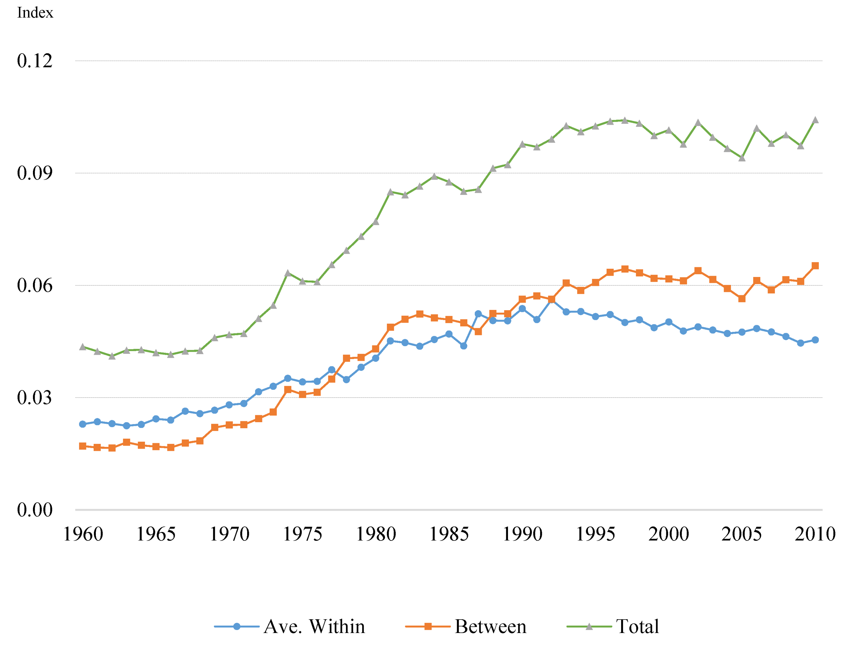
More interesting results are provided in Figure 4 calculated by Equation (6). Figure 4 reveals the total inequality with the between-region and the average within-region inequalities. The total inequality is the sum of the between-region and average-within inequalities. While the total inequality measures the nation-wide dispersion of CO₂ emissions, the between-region inequality represents the dispersion between regions, and the average-within inequality indicates the average inequality within regions. The total inequality increases from 0.04 to 0.10 over the period, but its increasing rate declines after early 1980s. The results show that CO₂ emissions continue to be distributed unequally in the U.S., but the extent to which CO₂ emissions diverge becomes stable after the U.S. launches ethanol usage in 1978. Although the total inequality is around zero, the results reveal that the extent to which the total inequality grows declines may be attributable to the use of ethanol.

Moreover, Figure 4 shows the increasing tendencies of the between and average-within inequalities over the period. The dispersion of CO₂ emissions becomes unequal between and within regions despite the low values around zero. From 0.02, the between and average-within inequalities increase to 0.07 and 0.05, respectively. The increasing rate of the between-region inequality is different from that of average within-region inequality. Like the total inequality, the between-region inequality rises at an increasingly rate between 1960s and 1980s, but its increasing rate starts declining after early 1980s. While the between-region inequality indicates that the dispersion of CO₂ emissions between regions increases over the period, the degree of its dispersion remains steady after early 1980s. In addition, the between-region inequality becomes higher than the average within-region inequality. The growth in the between-region inequality reveals a divergence of the distribution of CO₂ emissions between regions in the U.S., which is more likely to dominate the average within-region inequality.

The average within-region inequality also increases with an upward trend, but it starts decreasing around late 1980s. Compared with the between-region inequality that becomes more unequal, the average within-region inequality shows that the distribution of CO₂ emissions becomes more equal after late 1980s. In particular, the average-within inequality dominates the between-region inequality until mid 1980s, implying that the changes in the total the inequality are attributable mainly to the dispersion of CO₂ emissions among states within a region. However, the between and average-within inequalities diverge after mid 1980s, showing that the between-region inequality becomes greater than the average within-region inequality. While the extent to which CO₂ emissions disperse within a region declines, the between-region inequality begins increasing after mid 1980s, implying that the between-region inequality is more likely to contribute to the changes in the total the inequality than the average-within region inequality. The transformation of energy sources to ethanol may contribute to the changes in the between-region and average within-region inequalities, influencing the growth rate of the total inequality.

The trend changes in the inequalities occur around 1980s. To determine whether ethanol usage has a causal effect on the inequality changes, we estimate the econometric model constructed in Equation (7) using the generalized least squares with the bootstrapping method.

Table 2. Estimation Results.

	Average within Inequality	Between Inequality	Total Inequality
Ethanol-Fossil Fuel Ratio	−1.8379 ***	−1.7493 **	−2.5926 **
	(0.5302)	(0.7481)	(0.9886)
Time Trend	0.0009 ***	0.0014 ***	0.0018 ***
	(0.0001)	(0.0001)	(0.0001)
Constant	0.0213 ***	0.0117 ***	0.0343 ***
	(0.0010)	(0.0014)	(0.0020)
R-squared	0.86	0.94	0.92

Note: Bootstrapped standard errors are in parentheses. *** Denotes statistical significance at the 1% level. ** Denotes statistical significance at the 5% level.

reports the estimation results for the average within-region, the between-region, and the total inequalities, respectively. All the estimates are very similar. Specifically, the estimates for the time trend are positive and significant, which indicates that the extent to which the distribution of CO₂ emissions becomes unequal rises over time. The most interesting results are the estimates for the ratio of ethanol to fossil fuels. The estimates are negative and significant, which implies that an increase in the use of ethanol to fossil fuels is likely to reduce the inequalities of CO₂ emissions. The estimates for the average within-region, the between-region, and the total inequalities are −1.84, −1.75, and −2.59, respectively. The results are meaningful because the substitution of ethanol for fossil fuels contributes to the reductions in the inequalities of CO₂ emissions within and between regions.

The changes in the inequalities are associated closely with the substitution of ethanol for fossil fuels. Admittedly, the results imply that the reductions in the inequalities of CO₂ emissions are not necessarily beneficial for environment because they do not reflect the reductions in the absolute amounts of CO₂ emissions. However, according to the EPA, CO₂ emission coefficients vary with energy sources. While CO₂ emission coefficients measure how much fuel combustion generates CO₂, the coefficient of ethanol (0.068) is less than that of petroleum (0.073). As fossil fuels have been replaced with ethanol due to the U.S. ethanol policies, the reductions in the inequalities of CO₂ emissions may be an indicator of improving environmental conditions, implying that the use of ethanol contributes to the reductions in CO₂ emissions.

4. Conclusions

While a substantial combustion of fossil fuels has generated CO₂ emissions, regional climate conditions and energy-related activities have changed the distribution of CO₂ emissions across states in the U.S. Given the regional dispersion of CO₂ emissions, this study attempts to examine the differences in CO₂ emissions across nine climatically consistent regions within the contiguous U.S. This study offers the government with crucial information about the extent to which population growth contributes to CO₂ emissions under different weather conditions across the regions. Moreover, ethanol policy has been formulated to convert carbon energy to non-carbon energy. As the government now requires that ethanol be mixed with gasoline, this study also examines whether the use of ethanol is associated with the emission inequalities across the regions. This study provides economic implications of ethanol usage for reducing the regional inequalities of CO₂ emissions. As a reduction in the regional inequality of CO₂ emissions is associated with energy-related activities under different climate conditions, the transformation of energy sources into ethanol may be critical for achieving sustainable development. This study also contributes to providing stakeholders in the energy-related industry, local and national governments with useful information about ethanol usage relevant to the regional dispersion of CO₂ emissions.

The Theil’s entropy measure is used to examine the regional inequalities of CO₂ emissions. While CO₂ emissions per capita have increased over time, the results show that there exist regional variations in the nine within-region inequalities of CO₂ emissions. The overall within-region inequalities are around zero, but the northwest region has the lowest dispersion of CO₂ emissions, implying that there are less differences in CO₂ emissions across states within this region. The west north central region has the highest divergence of CO₂ emissions among the regions with a strong increasing rate, showing that the inequality in this region increases in proportion to an increase in the per-capita CO₂ emissions. More interestingly, the nation-wide dispersion defined by the total inequality increases over the sample period, but the increasing rate declines around early 1980s. The changes in the total inequality reflect the changes in the between-region and the average within-region inequalities. The between-region inequality increases at a decreasing rate, whereas the average within-region inequality begins to decrease around 1980s. The between-region inequality dominates the average within-region inequality, implying that the dispersion of CO₂ emissions becomes more unequal between regions rather than within regions.

The trend changes in the inequalities are relevant to the period of using ethanol. The econometric approach to examining the impact of ethanol usage on the inequalities yields meaningful results regarding the effects of ethanol usage on the emission inequalities. The results reveal that an increase in the ratio of ethanol to fossil fuels tends to reduce the inequalities of CO₂ emissions within and between regions, showing that the substitution of ethanol for fossil fuels contributes to the reductions in the inequalities of CO₂ emissions. Given the emission rate of ethanol, the use of ethanol is likely to reduce CO₂ emissions and their regional differences across regions. The findings offer significant policy implications. The findings relevant to the regional differences in CO₂ emissions can be used to formulate the nation-wide environmental policies. The policies can target the regions in which the regional dispersion is abnormal compared to other regions. Moreover, the findings reveal the importance of the conversion of carbon energy (i.e., fossil fuels) to non-carbon energy (i.e., ethanol). As the government encourages the substitution of ethanol for fossil fuels, the mandatory ethanol usage may reduce the differences in environmental qualities across regions along with associated energy and environmental policies. Due to the contribution of ethanol to the reductions in the emission inequalities, the mandatory ethanol usage may ultimately contribute to sustainable development in energy usage, thereby achieving environmental sustainability and improving energy security.