Abstract
This paper presents a study evaluating the perceptual similarity between artificial reverberation algorithms and acoustic measurements. An online headphone-based listening test was conducted and data were collected from 20 expert assessors. Seven reverberation algorithms were tested in the listening test, including the Dattorro, Directional Feedback Delay Network (DFDN), Feedback Delay Network (FDN), Gardner, Moorer, and Schroeder reverberation algorithms. A new Hybrid Moorer–Schroeder (HMS) reverberation algorithm was included as well. A solo cello piece, male speech, female singing, and a drumbeat were rendered with the seven reverberation algorithms in three different reverberation times (0.266 s, 0.95 s and 2.34 s) as the test conditions. The test was conducted online and based on the Multiple Stimuli with Hidden Reference and Anchor (MUSHRA) paradigm. The reference conditions consisted of the same audio samples convolved with measured binaural room impulse responses (BRIRs) with the same three reverberation times. The anchor was dual-mono 3.5 kHz low pass filtered audio. The similarity between the test audio and the reference audio was scored on a scale of zero to a hundred. Statistical analysis of the results shows that the Gardner and HMS reverberation algorithms are good candidates for exploration of artificial reverberation in Augmented Reality (AR) scenarios in future research.
1. Introduction
Artificial reverberation algorithms that can simulate a natural reverberation effect have continuously advanced since Schroeder first added a simulated room acoustic effect to a sound more than 60 years ago [1]. Such algorithms are applied in the field of virtual environments to simulate room acoustics and create convincing immersive experiences [2], for example, in augmented reality (AR) scenarios. AR is a technology that supplements the real world with virtual objects or scenes to make them appear to coexist in the same place as the real world [3]. If artificial reverberation is to be used in AR scenarios, it needs to meet the three properties of AR [3]:
- -
- Combining real and virtual objects in a real environment;
- -
- Running interactively and in real time;
- -
- Registering (aligning) real and virtual objects with each other.
These requirements emphasise the coexistence of virtual and real in the same space, the interactive alignment and mutual registration of virtual sources with physical reality and the real-time embeddedness (i.e., deviation from virtual reality) of AR, and its interactive nature [4]. Therefore, an artificial reverberation suitable for AR environments needs to be perceived as similar or the same as real reverberation, and react dynamically and in real-time.
Beginning in the 1960s, many artificial reverberation algorithms have been presented, the earliest and most famous being the reverberation algorithm presented by Schroeder [5]. Five popular reverberation algorithms presented by Moorer [6], Gardner [7], Jot [8], Dattorro [9], and Alary [10] are considered in this paper. A set of new binaural reverberation algorithms adapted from the Schroeder and Moorer reverberation algorithms are presented as well, with a linear structure that is simpler than the topology of Dattoro [9] and the feedback matrix structure of Alary [10]. The input audio enters through an FIR filter that simulates early reflections, and is output through a final all-pass filter without passing through a feedback loop [11].
In this paper, the seven aforementioned reverberation algorithms were implemented and the similarities between their perceived reverberation effects and measured binaural room reverberation were compared. A succinct review of reverberation algorithms applied to AR scenarios is presented before discussing each of the algorithms in depth. Section 2 presents the experimental materials, and methods and the results are presented in Section 3. Section 4 discusses the results, and Section 5 presents the conclusions of the study.
2. Background
2.1. Virtual vs. Real-World Acoustics
In an effort to establish appropriate reference conditions for this study, prior work which has looked at comparing real-world acoustic recordings with virtual acoustic rendering from acoustic measurements is first considered.
Kearney [12] compared the perceptual differences between actual acoustic recordings and ’virtual’ recordings made through convolution with binaural room impulse responses (BRIRs), which represent the transfer functions between a sound source and the ears as measured in a reverberant space. He assessed the differences between real and virtual violin and female speech recordings on five subjective attributes (source width, reverberance, clarity, naturalness and source movement). It was found that, apart from the source width, which is related to the directional response of the original acoustic source and the measurement loudspeaker, there was no significant difference between actual and virtual recordings in the other attributes [12]. The virtual acoustic recordings of the violin samples had a smaller source width. For the reverberance attribute, the samples did not differ statistically. For the clarity attribute, in the case of female singing, the virtual recording showed a significant improvement in clarity over the actual recording. For both source types, no variation in source movement was perceived overall. In terms of natural timbre, no significant differences were found between the actual and virtual source recordings.
Blau et al. [13] compared the various perceptual properties of real and auralised rooms in 2018. Their results showed that when using measured BRIRs, even non-individual BRIRs, highly convincing speech auralisation is possible. Small defects in the simulations can be reliably detected. Blau et al. [14] later compared the consistency of the auralisation of measurement-based binaural room impulse response with the real source (speech signal) for five attributes (reverberation, source width, source distance, source direction, and overall quality). The results showed that, although the measured BRIR set for ’reverberance’ was rated slightly lower than the other attributes with a median score of around 7 on a nine-point scale, for all other attributes, the agreement with the real room was rated with medians of 7.5 or higher on the nine-point scale based on the measured BRIR. The fact that the measured BRIR sets were capable of eliciting such high ratings suggests that the measured impulse response can be made realistically audible for speech. Therefore, it was concluded that close-to-real binaural auralizations of speech are possible if all modalities (auditory, visual, etc.) are appropriately reproduced [13]. Others, such as Lokki et al [15], have evaluated the properties of algorithmic simulations of binaural auralisation in relation to real head recordings. The results show that the spatial properties are almost identical, though there are differences in timbre. However, in general the auralisation algorithm achieves reasonable and natural binaural auralisation.
The perceptual similarity of real and virtual recordings reported in previous work therefore justifies the use of anechoic audio samples rendered with measured binaural room impulse responses as reference conditions to represent the ’real’ recorded reverberation in the current study.
It is important to note that the above experiments were all implemented in a static rendering environment and did not involve head tracking or testing in an augmented reality scenario.
2.2. Reverberation Algorithms for AR Scenarios
It is impractical to apply BRIRs measured in real spaces to AR scenarios, as AR can happen in any environment, requiring a large database of impulse responses to draw from, which is not as easy as manipulating the parameters of an algorithmic reverb [16]. Furthermore, measuring an impulse response is non-trivial, and multiple measurements are required for real-time interpolation if adaptive dynamic reverberation processing based on any user position is the goal [12,17].
There have been many significant efforts as of the time of writing in the application of computational reverberation algorithms for convincing AR.
Harma et al. proposed a technique and application of Wearable AR Audio (WARA) [18]. The model’s direct sound and 14 early reflections (six first-order and eight lateral planar second-order early reflections) were calculated from a simple shoebox room model with user-adjustable wall, floor, and ceiling positions. To match the length of the reverberation to that of the pseudo-acoustic environment, diffuse late reverberations were added using a variant of a Feedback Delay Network (FDN). The parameters of the reverberation algorithm (e.g. reverberation time) were set manually by analysing the reverberation of the environment or estimating parameters automatically from the binaural microphone signals. The additional information about the user’s orientation and position required for room modelling and binaural synthesis was estimated using a number of head-tracking devices.
A real-time binaural room modeling proposal for AR applications based on Scattering Delay Network (SDN) reverberation was presented by Yeoward, et al. in 2021 [19]. The combination of Digital Waveguide Network (DWN) and ray-tracing Image Source Method (ISM) approaches for SDN reverberation provides physical accuracy close to room simulation models while meeting the lower processing requirements of other reverberators that use delay networks [19,20,21]. A study by Djordjevic et al. [22] indicated that SDNs are considered more natural than binaural room impulse responses, ray tracing, and feedback delay networks in evaluations based on non-interactive simulations of two listening rooms. However, the suitability of SDNs for AR applications needs to be determined, as binaural SDN models have not been proposed in real-time architectures suitable for mobile or wearable computing devices [19].
Because this paper evaluates artificial reverberation algorithms based on delayed networks, SDN reverberation based on digital waveguide networks (DWN) and ray-traced image source models are not included among the studied algorithms. Moreover, the main disadvantage of computational acoustics is that the transfer operators take up a large memory footprint when sound propagates between surfaces, with the result that computational methods encounter a bottleneck [23,24].
Conversely, artificial reverberation algorithms based on delay network structures have flexible parameterization characteristics and better real-time performance [25]. It is useful to examine the output of such algorithms by looking at their response to a discrete unit sample function [26] passing through various filters and delay lines and feedback connections. This is equivalent to visualization of RIRs, and is readily achieved within the MATLAB environment [27], which has a rich filter structure database. In addition to recursive filters based on delay networks, simple finite impulse response (FIR) filters can be used to implement early reflection simulations. As a filter with no feedback support, FIR filters can be designed with arbitrary amplitude-frequency characteristics while maintaining strict linear phase characteristics, and are widely used in speech and data transmission [28]. However, because the filter has no feedback, more coefficients are required in the system equations [29]. For the purposes of AR, simplicity, real-time performance and computational efficiency must be considered.
In this context, the present paper is devoted to analysing the similarity between reverberation simulated with different delay networks against measured BRIRs.
For plausible AR scenarios, two channel binaural listening needs to be considered [30]. Binaural reverberation not only encapsulates room effects, it includes the cues for human sound source localisation, that is, inter-aural time and level differences and spectral cues due to the torso, head, and pinnae [31]. Therefore, the reverberation algorithms mentioned throughout this paper are binaural. In the case of measured reverberation, the BRIRs are impulse responses measured with a binaural dummy head.
2.3. Delay Network Reverberation
The traditional approach to synthesizing reverberation is based on delay networks combining feedforward paths to render early reflections and feedback paths to synthesize late reverberation [32]. One of the earliest and most famous reverberation algorithms was presented by Schroeder in 1961 [5]; it has a simple structure consisting of four parallel comb filters and two series all-pass filters, as shown in Figure 1 [27]. Natural reverberation consists of random closely-spaced impulse responses of exponentially decaying amplitude [33]. The first two conditions can be achieved by ensuring that the delay of each comb filter has no common divisor, and exponential decay can be achieved by making their reverberation times equal [5,8,34,35,36,37]. The reverberation time of the comb filters is equal to the overall reverberation time. Therefore, according to Schroeder’s recommendation [5,27], the maximum to minimum delay ratio of the four comb filters is approximately 1.5 (especially between 30–45 ms) and the gain of the comb filters are adjusted to obtain the desired reverberation time. The two all-pass filters have delays of approximately 5 ms and 1.7 ms, respectively, and their gains are both adjusted to 0.7. In this study’s implementation of Schroeder reverberation, the reverb time () is a user-oriented and adjustable parameter (range 0.1–5 s). The filter delays (T) are set according to Schroeder’s recommendations [5,27], and the filter gains (g) are calculated from the delay time (T) and the reverberation time () through Equation (1) [5]. The parameter values of each filter are presented in Table 1 [38].
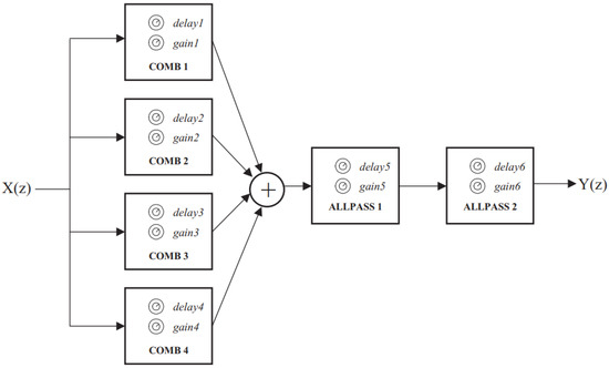
Figure 1.
The structure of Schroeder reverberation algorithm [27].

Table 1.
The parameter values of the Schroeder reverberation algorithm [38].
Moorer enhanced the Schroeder reverberation algorithm in 1979 [6] through four critical modifications, as shown in Figure 2 [39]. The first improvement was a Finite Impulse Response (FIR) delay line inserted in order to simulate the early reflections of the RIR. Another modification was inserting a one-pole low-pass filter into the feedback loop of each comb filter to simulate the absorption of sound by air in order to decrease the reverberation time at high frequencies, making the sound appear more real. Here, this is called the low-pass-feedback (LPF) comb filter. The third improvement was to increase the number of comb filters from four to six in order to obtain higher echo and modal density, especially for longer reverberation times. Finally, Moorer replaced the all-pass filter near the output with a delay filter to ensure that the late reflections arrive at the output a little later than the early reflections. Moorer proposed parameters for all filters in his study [6]. As in Schroeder’s reverberation algorithm, the random and closely spaced characteristics of pulses can be realized by ensuring that the delay of each comb filter has no common divisor, while the exponential attenuation can be realized by making its reverberation time () equal. Here, adjustments have been made to the parameters of the original low-pass comb reverberation filter. As in the Schroeder reverberation algorithm, the filter gain (g) is calculated from the delay time (T) and reverb time () through Equation (1). The FIR parameter values are presented in Table 2 [6]. The low-pass feedback gain values for all low-pass feedback comb filters are 0.9, and the values of the late reverberation filters are shown in Table 3 [6].
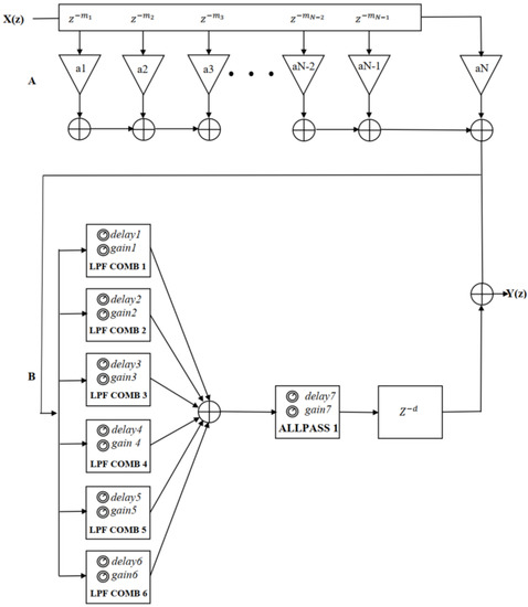
Figure 2.
The structure of Moorer reverberation algorithm [39], where the part A is the FIR delay line for simulating early reflections and the part B that is composed of six parallel low-pass-feedback comb filters, an all-pass filter and a delay filter is to simulate late reverberation.
Table 2.
The parameter values of the early FIR of the Moorer reverberation algorithm [6].
Table 3.
The parameter values of the the late reverberation filters of the Moorer reverberation algorithm [6].
Gardner proposed a set of reverberation algorithms aimed at simulating the reverberation effects of different room sizes [7]. These algorithms share three similar structures for different sizes of room (small, medium, and large) with different reverberation times [40]. These three reverberator structures are shown in Figure 3, Figure 4 and Figure 5, respectively [7,27], and their corresponding reverberation time ranges are presented in Table 4 [7]. The structures of these three algorithms mainly include all-pass filters (simple and nested), delay filters, and a first-order low-pass filter. In this study’s implementation of the Gardner reverberation, the delay length of each filter is adjusted somewhat to better match the correct reverberation time. The corresponding parameter values for each filter are presented in Table 5 [7].
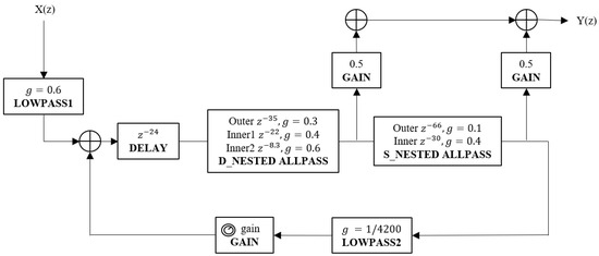
Figure 3.
The structure of the Gardner reverberation algorithm for small size room [7].
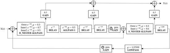
Figure 4.
The structure of the Gardner reverberation algorithm for medium size room [7].
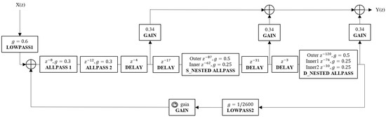
Figure 5.
The structure of the Gardner reverberation algorithm for large size room [27].
Table 4.
The corresponding reverberation time ranges for each Gardner reverberator [7].
Table 5.
The parameter values of the the late reverberation filters of the Gardner reverberation algorithm [7].
Feedback Delay Network (FDN) was proposed by Jot in 1992 [8]. It consists of N-dimensional delay lines and a feedback matrix, as shown in Figure 6 [10,27,41]. As a novel and versatile reverberator design structure, it provides separate and independent control of the energy storage, damping, and diffusion components of the reverberator [42]. Compared with parallel comb filters, this feedback structure can generate much higher echo density given a sufficient number of non-zero feedback coefficients and delay lengths [41]. In this paper, we adopt four-dimensional delay lines. In this structure, following Schroeder’s advice [5], the delay length () of each delay line is derived from a prime power exponential delay Equations (2) to (5). The gain () for each delay line is calculated from a given reverberation time () and sample rate () by Equations (6) to (8) according to Alary’s [10] suggestion. The feedback matrix (A) is implemented by a fourth-order Hadamard matrix. The input gain (), output gain (), and direct sound gain (d) are all set as 1 in this structure, and can be adjusted as required. The total minimum delay length is defined as
where indicates plus one for rounding; is the preliminary estimate of the non-prime-number delay length for each delay line, and is expressed as
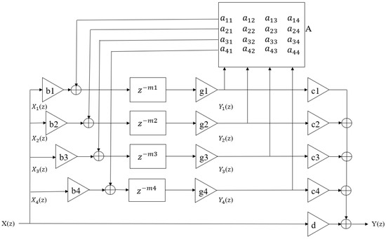
Figure 6.
The structure of Feedback Delay Network (FDN) [10,41], where the part A represents the feedback coefficient matrix.
is the index of the position of the prime number to be drawn from the set of prime numbers, given by
where prime is 2, 3, 5, 7, 11, etc., means rounding to the nearest whole number, and is the delay of each delay line, which is a power of a distinct prime provided by
is a per-sample attenuation gain, is a linear scale gain converted from a logarithmic scale gain, and is the target gain of each delay line, given respectively as
Dattorro published a topology structure for a reverberation algorithm in 1997 [9]. The implementation of this reverberation structure is composed of a pre-delay followed by a low-pass filter, a decorrelation stage, and a ‘tank implementation’, as shown in Figure 7 [27]. The decorrelation stage includes four cascaded all-pass filters which can perform a rapid build-up of echo density. The decorrelation stage does not have a feedback loop, and as such is straightforward; however, the ‘tank’ is more complex because of its recursive structure [27]. The ‘tank implementation’ consists of two cross-coupled symmetrical lines, which cause the infinite recirculation of the input signal. Each line contains two all-pass filters, two delays, a low-pass filter, and two decay coefficients for attenuation. These decay coefficients help to control the reverberation time. The input signal passes through these filtering structures accordingly, and the network produces a final decorrelated all-wet stereo output by summing up six output signals extracted from the ‘tank implementation’ [27]. The delay length is marked in Figure 7 [27]; the delay of the pre-delay is 0.001 s, the decay is derived from a given reverberation time () and sample rate () by Equations (9) to (12), and the other parameters used in this structure are presented in Table 6 [27]. In addition, the delays and signs used to generate the output of Dattoro’s reverberator are provided in Table 7 [27].
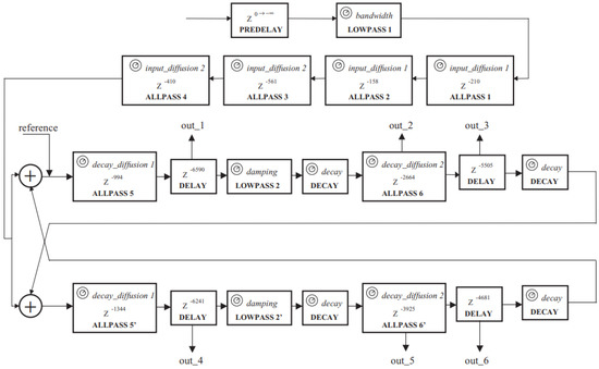
Figure 7.
The structure of the Dattorro reverberation algorithm [27].
Table 6.
The parameters of the Dattorro reverberation algorithm [27].
Table 7.
Delays and signs used to generate the output of Dattoro’s reverberator [27].
Alary designed a new reverberation algorithm named the Directional Feedback Delay Network (DFDN) in 2019, which is shown in Figure 8 [10]. The DFDN is an extension of a conventional FDN, which can produce direction-dependent reverberation times and control the energy decay of a reverberant sound field, which is suitable for anisotropic decay reproduction on a loudspeaker array or in binaural playback through the use of Ambisonics [10]. Considering computational cost, the higher the order of the Ambisonics, the longer the running time. When comparing the computational cost with a traditional FDN, the cost of the DFDN increases by a factor equal to the number of channels in the delay line group. For example, a four delay-line DFDN using third-order Ambisonics was adopted by Alary [10]; thus, his reverberator has four groups of sixteen delay lines, making for a total of 64 delay lines. Therefore, the number of delay lines increases by a factor of 16 when compared to an equivalent conventional FDN. However, the DFDN used in this paper adopts four delay lines using first-order Ambisonics in order to reduce computational costs. First-order Ambisonics includes four channels, meaning that the reverberator has four groups of four delay lines, making for a total of sixteen delay lines, which decreases the number of delay lines by a factor of four compared to an equivalent third-order Ambisonics DFDN. The parameters and simulation of this reverberation algorithm can be found in Alary’s research [10].
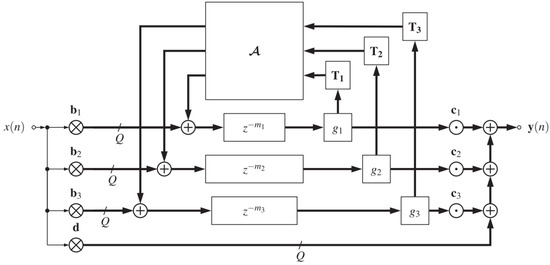
Figure 8.
Structure of Direction Feedback Delay Network (DFDN) [10].
2.4. Hybrid Moorer–Schroeder Implementation
In this paper, we propose a new reverberation algorithm which combines and modifies the Schroeder and Moorer reverberation algorithms, with the aim of simulating the reverberation effects of different sized rooms. This algorithm is referred to as the Hybrid Moorer–Schroeder (HMS) reverberation algorithm in this paper. The HMS reverberation algorithm simulates the reverberation of rooms of different sizes (small, medium, and large) by varying the filter coefficients in the internal structure depending on different reverberation time ranges.
2.4.1. The Basic Mono Structure of the HMS Reverberation Algorithm
The reverberation structures of the algorithm are shown in Figure 9. The filter coefficients in the dashed boxes change according to the reverberation time range shown in Table 4, and the lower limit of the time range for small-size-room reverberator is 0. The structures of the HMS algorithm mainly include an FIR delay line, comb filters, low-pass-feedback comb filters, all-pass filters, delay filters, and first order low-pass filters.
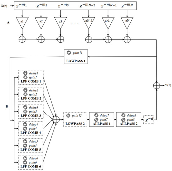
Figure 9.
The structure of the HMS reverberation algorithm, where the part A is the FIR delay line for simulating early reflections and the part B that is composed of different filters is to simulate late reverberation.
The large-room HMS reverberation algorithm was modified by inserting a one-pole low-pass filter following the FIR delay line in the Moorer reverberation algorithm [6] to filter the high-frequency noise to smooth the audio [43]. Another all-pass filter was inserted between the all-pass filter and the delay filter to increase the number of echoes from the comb filter output and ensure that their phase characteristics cause minimal interference [27,44]. Meanwhile, a further low-pass filter was added following the parallel low-pass-feedback comb filters to further reduce the high-frequency noise and simulate the air absorption [6,43]. The parameter values of the FIR are the same as those for the Moorer reverberation algorithm shown in Table 2 [6]. The gain values of low-pass filters 1 and 2 are 0.6 and 0.3, respectively. The low-pass feedback gain values for all low-pass feedback comb filters are 0.9. The parameter values of the other late reverberation filters are presented in Table 8.
Table 8.
Parameter values of the the late reverberation filters of the HMS reverberation algorithm for large and medium room sizes.
The medium-room HMS reverberation algorithm was achieved by setting the gain (g) and delay coefficients () of low-pass filter 2 to zero in the large-room HMS reverberation algorithm, as shown in Figure 10, effectively removing it from the algorithm. A study by Harris et al. [45] indicated that the attenuation constant of air is usually important only in large rooms or at high frequencies; thus, further simulation of high frequency noise attenuation and air absorption is not necessary in medium and small rooms. The parameter values of the FIR are same as those for the Moorer reverberation algorithm shown in Table 2 [6]. The gain value of low-pass filter 1 is 0.55. The gain value of the low-pass feedback of all low-pass-feedback comb filters is 0.9. The parameter values of the other late reverberation filters are presented in Table 8.
Figure 10.
The structure of the low-pass filter in the large-room HMS reverberation algorithm.
The small-room HMS reverberation algorithm was improved by adding a Finite Impulse Response (FIR) delay line and a one-pole low-pass filter following the FIR delay line before the Schroeder reverberation algorithm [5]. Therefore, as in the medium-room HMS algorithm, the coefficients of low-pass filter 2 were set to zero in the large-room HMS algorithm, as shown in Figure 10. Furthermore, all gain (g and ) and delay coefficients ( and ) of low-pass-feedback comb filters 5 and 6 were set to zero, as shown in Figure 11, disabling low-pass-feedback comb filters 5 and 6. The gain () and delay coefficients () of the low-pass feedback section of low-pass feedback comb filters 1 to 4 were set to zero as well, as shown in Figure 11. This means that low-pass-feedback comb filters 1 to 4 were converted to comb filters 1 to 4, as shown in Figure 12. The coefficient of the delay filter was set to zero, meaning that it does not function. The parameter values of FIR are the same as for the Moorer reverberation algorithm shown in Table 2 [6]. The gain value of low-pass filter 1 is 0.3. The parameter values of the other late reverberation filters are presented in Table 9.
Figure 11.
The structure of the low-pass feedback comb filter in the large-room HMS reverberation algorithm.
Figure 12.
The structure of the comb filter in the large-room HMS reverberation algorithm.
Table 9.
Parameter values of the the late reverberation filters of the HMS reverberation algorithm for small rooms.
2.4.2. The Binaural Optimised Structure of Reverberation Algorithms
In order to realise binaural audio, all reverberation algorithms mentioned in Section 2.3 and Section 2.4.1 were optimised with two channels to generate binaural reverberation, as shown in Figure 13. Here, the mono input is the output of the above seven reverberation algorithms. First, the above mono structures are regarded as the left channel of the binaural reverberation algorithm, and the difference between right channel and left channel is achieved through a random constant as the delay parameter (). The parameter is set to 0.1 in this paper, though it can be adjusted. The filter delay parameters for the right channel reverberation structure are implemented by Equation (13):
where is the delay parameter for all filters in the right channel, is the delay parameter for all filters in the left channel, and is the random delay parameter mentioned above.
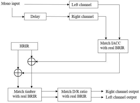
Figure 13.
Structure of the binaural reverberation algorithm.
Next, the Interaural Cross-correlation Coefficient (IACC) of the left channel and the right channel are matched with a measured BRIR through a channel correlation parameter () as Equation (14). Interaural Cross-Correlation is a measure of the difference between the signals received by a person’s two ears that measures the spaciousness of the listening room and the listener’s envelopment [46]. Large IACC values correspond to greater degrees of envelopment and a more enjoyable overall listening experience in auditoriums [47].
where is the output binaural impulse response (two columns) from reverberation algorithms, is the flip column of the output binaural impulse response around the vertical axis in the left–right direction, is the output binaural impulse response after matching IACC, and is the channel correlation parameter mentioned above.
The minimum phase reconstructed version of the 0 degree azimuth and 0 degree elevation HRIR from Subject D1 of the SADIE II database is added as the direct sound component [48]. The minimum-phase version is taken to ensure the energy of the impulse response is moved to the start of the filter, implemented via the rceps function in MATLAB.
The timbre of the reverberation is then matched to the measured BRIR. Timbre matching is performed separately for the left and right channels, and is only performed on the reverberation, not on the direct sound. IRs from the reverberators are extracted and the root mean square value in Equivalent Rectangular Bandwidth (ERB) bands is compared to the measured IR using a 4096 tap ERB linear phase filter bank with 24 bands. The difference in each band is then computed and the algorithmic reverb is scaled by the difference. Outputs from the filterbank are then summed and the direct sound is added.
Finally, the direct-to-reverberant (D/R) energy ratio of the impulse response generated by the reverberation algorithm is matched with the measured BRIR. The original D/R energy ratio of the impulse response generated by the reverberation algorithm is first found by Equation (15), then its reverberation portion is scaled by Equation (16) to match the D/R energy ratio of the desired measured impulse response. The direct-to-reverberant (D/R) energy ratio can then be used as an acoustic cue in a reflective environment in relation to a one-to-one distance, avoiding confusion with source characteristics [49]. In a typical listening room, the direct sound field energy decays proportionally to the (logarithmic) distance, while the energy of the reverberant sound field is independent of the distance. Therefore, D/R can in principle be used to estimate the distance of a sound source [50].
where is the original D/R energy ratio of the impulse response generated by the reverberation algorithm, represents the average of the left and right channels, represents the calculation of the root mean square, represents the direct sound portion, and represents the reverberation portion:
where is the scaled reverberation portion, is the original reverberation portion, and represents the D/R energy ratio of desired measured impulse response.
3. Materials and Methods
A listening test based on the Multiple Stimuli with Hidden Reference and Anchor (MUSHRA) paradigm [51] was designed to evaluate the similarity between the artificial reverberation algorithms and measured reverberation. Here, similarity represents the closeness of timbre and perceived reverberation. A scale of zero to one hundred was adopted. The reference condition is set as the standard and a test condition that is perceived as the same as the reference condition is scored as 100.
3.1. Test Materials and Reference Binaural Room Impulse Responses
The seven reverberation algorithms defined in Section 2.3 and Section 2.4.1 were used in the listening test, and each algorithm was binauralized according to the method in Section 2.4.2. The test materials consisted of commonly used male speech, female singing, a solo cello piece, and a drumbeat [52], each rendered with the seven different reverberation algorithms with three different reverberation times (0.266 s, 0.95 s, and 2.34 s). Jouni Paulus et al. used these same materials as part of their experimental material when studying the perceived level of late reverberation in speech and music [53]. The four audio samples were chosen for the following reasons:
- -
- Male speech is a common and recognised sound source with a familiar timbre.
- -
- Female singing is a familiar musical source with less energy at low frequencies.
- -
- A solo cello piece is used as a low frequency source.
- -
- A drumbeat is used as an example of more transient sounds.
These four test materials are all one-channel anechoic audio of 10 s length with 44.1 kHz sample rate and 24 bits bit depth.
The reference conditions are obtained by the four audio samples rendered with measured BRIRs with the three different reverberation times.
In each trial, there are nine stimuli: seven stimuli convolved with different BRIRs generated by seven different reverberation algorithms, one hidden reference, and one low anchor (dual-mono 3.5 kHz low pass filtered audio), for a total of 108 stimuli and 12 trials in the whole listening test.
The BRIR with 0.266 s reverberation time, shown in Figure 14a, was measured from Control Room 7 at WDR Broadcast Studios, Germany. It was taken using a KU100 at 3 m from the source [54]. The BRIR with 0.95 s Reverberation time, shown in Figure 14b, was measured from the Printing House Hall at Trinity College Dublin, Ireland. It was obtained using a KU100 at 2 m from the source [55]. The BRIR with 2.34 s Reverberation time, shown in Figure 14c, was measured from the Lady Chapel at St Alban’s Cathedral, United Kingdom. It was taken using a KU100 at 4.2 m from the source [56]. A comparison of IACC and D/R energy ratio between the measured BRIRs and BRIRs generated from the reverberation algorithms is presented in Table 10. The IACCs of all BRIRs generated by the reverberation algorithm are matched as closely as possible to the IACCs of the measured BRIRs, and all the D/R energy ratios have been matched exactly.
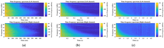
Figure 14.
The spectrograms of the BRIRs used in the listening test: (a) BRIR with 0.266 s reverberation time, (b) BRIR with 0.95 s reverberation time, and (c) BRIR with 2.34 s reverberation time.
Table 10.
Comparison of IACC and D/R energy ratio between measured BRIRs and BRIRs generated from reverberation algorithms.
3.2. Experimental Design
The whole listening test was built on the WebMUSHRA online platform [51]. The participants were informed of the purpose of the experiment and the protocol of the experiment prior to conducting their trial on the online platform. After participants reviewed the information sheet and agreed the consent form, they could access the whole listening test via a WebMUSHRA URL. At the end of the listening test, demographic information such as email, type of headphone used, age, and gender were collected. This study was approved by the University of York Physical Sciences Ethics Committee (approval code: Mi070821).
A training session was conducted before the test, where participants could set a safe and comfortable headphone listening level, read the description carefully, and familiarize themselves with the user interface.
Participants were asked to listen to the reference audio and each stimulus carefully and to judge the similarity between each stimulus and the reference audio sample on a scale of zero to a hundred. The stimulus which was the same as the reference audio sample was expected to score a hundred, and the more similar the other stimuli were to the reference audio sample, the higher the expected score.
3.3. Subjects
A total of 26 participants completed the test. Twenty of these were selected as expert listeners and experienced assessors according to the post-screening of assessors in ITU-R BS.1543-3 recommendation [57]. Six of the participants who did not meet this criteria were excluded. Each participant was paid to take part in the test, which lasted about 40 min. All participants were between 20 and 60 years old; ten identified as male and ten as female. All of these participants were members of York AudioLab or music-related majors at the University of York or Beijing Film Academy.
3.4. Design Limitations
Due to the COVID-19 pandemic, this listening was conducted remotely online; thus, the listening environment, type of headphones (although Beyerdynamic DT990 was advised), and volume of audio samples were dependent on the preference of the test subjects. The headphone types used in this experiment included seven Beyerdynamic DT990, two BeyerDynamic DT770, two Beyerdynamic DT240, two ATH-M50x, two AKG K701, one QDC Anole V6, one Audeze LCD-X, one Harman AKG N60NC (plugged in), one NEUMANN NDH20, and one Sony MDR7506. A significance test between the Beyerdynamic DT990 and other headphones was carried, out, with the results shown in Table A1 in Appendix A. No significant differences were observed between the Beyerdynamic DT990 and other headphones; thus, no particpants were excluded based on the type of headphones.
The COVID-19 pandemic imposed limitations on the search for voluntary participants. Finding a large number of people to participate in studies remotely was difficult; thus, the experiment analysed a sample of only about 20 participants. According to ITU-R BS.1543-3 recommendation [57], in a situation where listening test conditions are tightly controlled in terms of both technique and performance previous experience has shown that data from no more than 20 evaluators may be sufficient to draw appropriate conclusions from the test. Therefore, it is justifiable for this experiment to analyse a sample of only about 20 participants.
4. Results
In this experiment, the average score of the reverberation algorithms was used as a criterion for judgment. The higher the score, the better the simulation effect. After all the results were collected, box plots were used to detect outliers. The data were then subjected to mean analysis to determine which algorithm scored the highest and was the most similar to the real reverberation. This was followed by a significance test and a post hoc test to check whether there were significant differences between the algorithms. In addition, the processing times of each reverberation algorithm were analysed to compare their computational costs.
4.1. Mean Value Analysis
Box plots were used to detect the outliers from the raw data, defined as the values outside the upper and lower quartiles plus 1.5 times the interquartile range [58]. Figure 15, Figure 16, Figure 17 and Figure 18 show box plots of the scores for the seven reverberation algorithms, reference (Ref), and anchor applied to female singing, male speech, cello piece, and drumbeat with 0.266 s, 0.95 s, and 2.34 s reverberation times, respectively. As these outliers were not identified as input or measurement errors and the listening test was based on a subjective evaluation, these outliers were retained and analysed using non-parametric hypothesis tests to ensure robustness.
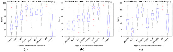
Figure 15.
Box plots of the scores of seven reverberation algorithms, reference and anchor simulating female singing, male speech, cello piece, and drumbeat with 0.266 s, 0.95 s, and 2.34 s reverberation time: (a) 0.266 s, (b) 0.95 s, (c) 2.34 s (’+’ in figures presents outliers).
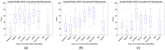
Figure 16.
Box plots of the scores of the seven reverberation algorithms, reference, and anchor simulating male speech with 0.266 s, 0.95 s, and 2.34 s reverberation time: (a) 0.266 s, (b) 0.95 s, (c) 2.34 s (’+’ in figures presents outliers).
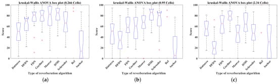
Figure 17.
Box plots of the scores of the seven reverberation algorithms, reference, and anchor simulating cello piece with 0.266 s, 0.95 s, and 2.34 s reverberation time: (a) 0.266 s, (b) 0.95 s, (c) 2.34 s (’+’ in figures presents outliers).
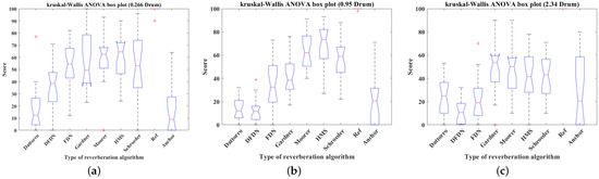
Figure 18.
Box plots of the scores of the seven reverberation algorithms, reference, and anchor simulating drumbeat with 0.266 s, 0.95 s, and 2.34 s reverberation time: (a) 0.266 s, (b) 0.95 s, (c) 2.34 s (’+’ in figures presents outliers).
The data provided by these 20 experienced participants were then averaged to determine which algorithm was perceived as having reverberation most similar to the real reverberation. Figure 19a–c present the mean score with standard error of the female singing simulated by reverberation algorithms under short (0.266 s), medium (0.95 s), and long (2.34 s) reverberation times. Similarly, Figure 20a–c, Figure 21a–c, and Figure 22a–c present the same data for the male speech, cello piece, and drumbeat, respectively.
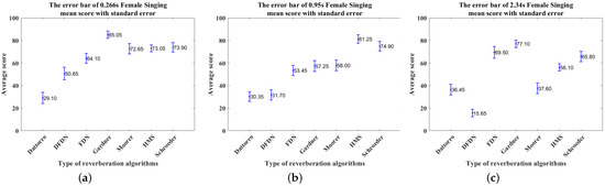
Figure 19.
The error bars of the mean score with standard error of the female singing simulated by the reverberation algorithms under short (0.266 s), medium (0.95 s), and long (2.34 s) reverberation times: (a) 0.266 s, (b) 0.95 s, (c) 2.34 s.
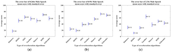
Figure 20.
The error bars of the mean score with standard error of the male speech simulated by the reverberation algorithms under short (0.266 s), medium (0.95 s), and long (2.34 s) reverberation times: (a) 0.266 s, (b) 0.95 s, (c) 2.34 s.
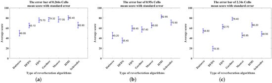
Figure 21.
The error bars of the mean score with standard error of the cello piece simulated by the reverberation algorithms under short (0.266 s), medium (0.95 s), and long (2.34 s) reverberation times: (a) 0.266 s, (b) 0.95 s, (c) 2.34 s.
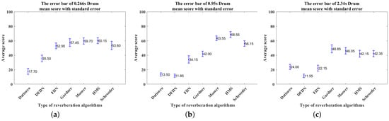
Figure 22.
The error bars of the mean score with standard error of the drumbeat simulated by the reverberation algorithms under short (0.266 s), medium (0.95 s), and long (2.34 s) reverberation times: (a) 0.266 s, (b) 0.95 s, (c) 2.34 s.
The mean scores of the above reverberation algorithms are listed in Table 11. The highest scores are shown in bold and are concentrated among the Gardner and HMS reverberation algorithms. In general, the Gardner reverberation algorithm’s simulation of long reverberation is perceived as closer to the real reverberation. The HMS reverberation algorithm generally performs better in the simulation of medium and short reverberation times, except for the female singing in the short reverberation time, where the Gardner reverberation algorithm outperforms the HMS algorithm.
Table 11.
The mean scores of the above reverberation algorithms simulating the female singing, male speech, cello piece, and drumbeat at short (0.266 s), medium (0.95 s), and long reverberation times (2.34 s), respectively.
4.2. Statistical Analysis
4.2.1. Non-Parametric Kruskal–Wallis One-Way ANOVA Test
Listening test data were checked for normality and variance homogeneity using the Lilliefors test [59] and Bartlett test [60]. The results show that not all data conform to normal distribution and homogeneity of variance. In addition, because of the presence of outliers and in order to ensure robustness, a non-parametric Kruskal–Wallis one-way ANOVA test [61] with 95% confidence intervals [62] was run to determine whether there were significant differences between the seven reverberation algorithms. The results are presented in Table 12. The null hypothesis was that there were no significant differences between the seven reverberation algorithms. All p-values were less than the significance level of 0.05; thus, the null hypothesis is rejected, meaning that there are significant differences between the seven reverberation algorithms.
Table 12.
Kruskal–Wallis ANOVA test results for all seven reverberation algorithms.
4.2.2. Post Hoc Test
Post hoc tests were performed to confirm where differences between groups occurred. Pairwise Comparison in Multiple Comparison was performed to determine which two groups were significantly different from each other. The post hoc test results reveal whether the highest-scoring reverberation algorithm is significantly different from the other reverberation algorithms.
Table 13, Table 14 and Table 15 present the Pairwise Comparison post hoc test results. The values presented in Table 13, Table 14 and Table 15 are p-values. Those p-values less than 0.05 indicate significant differences.
Table 13.
Post hoc test results for short reverberation time (0.266 s).
Table 14.
Post hoc test results for medium reverberation time (0.95 s).
Table 15.
Post hoc test results for long reverberation time (2.34 s).
As described in Section 4.1, the algorithms with the highest scores are shown in bold in Table 11. Reverberation algorithms that are not significantly different from the highest scoring reverberation algorithm are marked in bold italics in Table 11.
It can be seen that at short reverberation times, although HMS achieved the highest scores in simulating all three stimuli except female singing, overall there were no significant differences between the HMS, Gardner, and Schroeder reverberation algorithms in simulating the four stimuli in the experiment. At medium reverberation times, there was no significant difference between the HMS and Schroeder reverberation algorithms, although HMS scored highest when simulating real reverberation. At long reverberation times, the Gardner reverberation algorithm performed best.
4.3. Computational Cost Analysis
The processing overhead for each reverberation algorithm was extracted through the Profiler in MATLAB, with the results listed in Table 16. The comparison shows that DFDN is far less computationally efficient than the other algorithms. At low reverberation times, Schroeder, Gardner, and FDN have the lowest computational costs. At medium reverberation times, the Schroder and Gardner algorithms are more computationally efficient than the others. At long reverberation times, the Schroeder and Moorer reverberation algorithms are far more computationally efficient than the others, followed by the Gardner algorithm, which is slightly more computationally efficient than the rest. The computational cost of our proposed HMS reverberation algorithm is slightly higher than the Gardner, Moorer, and Schroeder algorithms.
Table 16.
Computational cost of the seven reverberation algorithms at three different reverberation times.
4.4. Results Summary
In this experiment, a reverberation algorithm is considered good when it scores 60 or more, and excellent when it scores 80 or more [57].
The experimental results showed that HMS scored highest in simulating all three stimuli except for the female singing at the shorter reverberation time. The HMS and Gardner reverberation algorithms scored highest at the medium reverberation time and long reverberation time, respectively. However, non-parametric ANOVA tests and post hoc tests of the above data showed that the Gardner reverberation algorithm’s simulations were closer to the real perceptual reverberation during the long reverberation time, while the HMS and Schroeder reverberation algorithms’ simulations were better during the short and medium reverberation times. HMS performed well in terms of the twelve stimuli overall, as HMS obtained the seven highest scores out of the twelve stimuli tested. In addition, there was no significant difference between HMS and the highest scoring reverberation algorithm in eleven stimuli, with the exception being the female singing with long reverberation. The Schroeder reverberation algorithm was second best, as except for male speech and cello piece with long reverberation condition there was no significant difference between the Schroeder reverberation algorithm and the reverberation algorithm that scored highest in ten stimuli. Furthermore, the Schroeder reverberation algorithm has the lowest computational cost compared to the rest.
5. Discussion
Our experimental results indicate that the Schroeder algorithm is the better choice if perceptual performance is not particularly important and computational efficiency is required. If computational efficiency is not particularly important and perceptual performance is a concern, the HMS reverberation algorithm might be preferable. Alternatively, a combination of the Schroeder and Gardner reverberation algorithms or the HMS and Gardner reverberation algorithms, with Schroeder and HMS for short and medium reverberation times and the Gardner reverberation algorithm for long reverberations, might be beneficial.
It is interesting to note that of the four audio samples, the scores for the male speech and the drumbeat are generally lower than those for female singing and cello piece. The scores for the drumbeat are particularly low. Therefore, the results suggest that the artificial reverberation algorithms tested in this experiment are less successful in simulating percussive sounds to make their perceptual effects similar to real reverberation. Frissen et al. [63] showed that although stimulus type has no effect on the ability to discriminate reverberation, this does not mean that the absolute amount of perceived reverberation is the same for different types of stimuli. Their study found that speech stimuli led to higher estimates of reverberation than singing or drums. This was particularly true for relatively long reverberation times (i.e., >1.8 s). Moreover, the absolute amount of perceived reverberation for drums was significantly different from that for vocal stimuli (include speech and singing). Thus, sound stimulus can have an effect.
This is due to the fact that remote experiments conducted under COVID-19 restrictions could affect the listener’s perception of the stimuli; thus, it is important to confirm the findings with in-person testing in further studies. It should be noted that this experiment is a static binaural reverberation parameter test rather than a dynamic one. However, the static case provides a valuable foundation before attempting fully head-tracked AR scenario conditions.
6. Conclusions
This experiment evaluated the similarity between different artificial reverberation algorithms and measured reverberation, including the assessment of a novel reverberation algorithm, the HMS. The motivation for the study was to consider the suitability of reverberation algorithms to be applied to AR scenarios in the future to create more plausible reverberation effects. In the long reverberation time, the simulation of the Gardner reverberation algorithm was perceived as closer to the measured perceptual reverberation, while the simulation of HMS and Schroeder reverberation algorithms were more similar in the short and medium reverberation times. In addition, across all twelve stimuli, the HMS reverberation algorithm obtained the seven highest scores in the twelve stimuli tested. Except for the female singing in the long reverberation, there was no significant difference between the HMS reverberation algorithm and the reverberation algorithm with the highest score in the other eleven stimuli. The Schroeder reverberation algorithm is a good choice if perceptual performance is not particularly important and computational efficiency is required. Alternatively, based on the absolute advantage of the Gardner reverberation algorithm in simulating real reverberation under long reverberation times, a combination of HMS and Gardner or Schroeder and Gardner algorithms could be a way forward for AR scenes.
Future work should investigate the combination of the Gardner and HMS reverberation algorithms into a set of algorithms that simulate room models with different reverberation times using head tracking and an AR framework to realise dynamic reverberation.
Author Contributions
Conceptualisation, H.M. and G.K.; methodology, H.M., G.K. and H.D.; software, H.M.; validation, H.M.; formal analysis, H.M.; investigation, H.M.; resources, H.M., G.K. and H.D.; data curation, H.M.; writing—original draft preparation, H.M.; writing—review and editing, G.K. and H.D.; visualization, H.M.; supervision, G.K. and H.D.; project administration, H.M. funding acquisition, G.K. All authors have read and agreed to the published version of the manuscript.
Funding
This research was supported by the Engineering and Physical Sciences Research Council IAA project “MINERVA: Musical Interactions in Networked Experiences using Real-time Virtual Audio”.
Institutional Review Board Statement
The study was conducted according to the guidelines of the Declaration of Helsinki, and approved by the Ethics Committee of University of York (protocol code Mi070821 and 9 August 2021 of approval).
Informed Consent Statement
Informed consent was obtained from all subjects involved in the study. Written informed consent has been obtained from the patient(s) to publish this paper.
Data Availability Statement
The data presented in this study are available in insert article.
Conflicts of Interest
The authors declare no conflict of interest.
Abbreviations
The following abbreviations are used in this manuscript:
| AR | Augmented Reality |
| BRIR | Binaural room impulse response |
| DFDN | Directional Feedback Delay Network |
| D/R | Direct-to-reverberant |
| ERB | Equivalent Rectangular Bandwidth |
| DWN | Digital Waveguide Networks |
| FDN | Feedback Delay Network |
| FDTD | Finite-difference Time-Domain |
| FIR | Finite impulse response |
| FTP | File Transfer Protocol |
| HMS | Hybrid Moorer-Schroeder |
| HRTFs | head related transfer functions |
| IACC | Interaural Cross-correlation Coefficient |
| ISM | Image Source Mode |
| LPF | Low pass feedback |
| MUSHRA | Multiple Stimuli with Hidden Reference and Anchor |
| RIR | Room impulse response |
| SDN | Scattering Delay Network |
| WARA | Wearable Augmented Reality Audio |
Appendix A
Table A1.
The ANOVA test results between Beyerdynamic DT990 and other headphones.
Table A1.
The ANOVA test results between Beyerdynamic DT990 and other headphones.
| DF = 1 Significance Level = 0.05 | p Value |
|---|---|
| 0.266 s female singing | 0.875 |
| 0.266 s male speech | 0.057 |
| 0.266 s cello piece | 0.614 |
| 0.266 s drumbeat | 0.358 |
| 0.95 s female singing | 0.125 |
| 0.95 s male speech | 0.664 |
| 0.95 s cello piece | 0.064 |
| 0.95 s drumbeat | 0.206 |
| 2.34 s female singing | 0.130 |
| 2.34 s male speech | 0.093 |
| 2.34 s cello piece | 0.474 |
| 2.34 s drumbeat | 0.545 |
References
- Välimäki, V.; Parker, J.; Savioja, L.; Smith, J.O.; Abel, J. More than 50 years of artificial reverberation. In Proceedings of the Audio Engineering Society Conference: 60th International Conference: Dreams (Dereverberation and Reverberation of Audio, Music, and Speech), Audio Engineering Society, Leuven, Belgium, 3–5 February 2016. [Google Scholar]
- Gardner, W.G. Reverberation algorithms. In Applications of Digital Signal Processing to Audio and Acoustics; Springer: Berlin/Heidelberg, Germany, 2002; pp. 85–131. [Google Scholar]
- Azuma, R.; Baillot, Y.; Behringer, R.; Feiner, S.; Julier, S.; MacIntyre, B. Recent advances in augmented reality. IEEE Comput. Graph. Appl. 2001, zoo, 34–47. [Google Scholar] [CrossRef]
- Javornik, A. Augmented reality: Research agenda for studying the impact of its media characteristics on consumer behaviour. J. Retail. Consum. Serv. 2016, 30, 252–261. [Google Scholar] [CrossRef]
- Schroeder, M.R. Natural sounding artificial reverberation. In Proceedings of the Audio Engineering Society Convention 13, Audio Engineering Society, New York, NY, USA, 9 October 1961. [Google Scholar]
- Moorer, J.A. About this reverberation business. Comput. Music. J. 1979, 3, 13–28. [Google Scholar] [CrossRef]
- Gardner, W.G. The Virtual Acoustic Room. Ph.D. Thesis, Massachusetts Institute of Technology, Cambridge, MA, USA, 1992. [Google Scholar]
- Jot, J.M.; Chaigne, A. Digital delay networks for designing artificial reverberators. In Proceedings of the Audio Engineering Society Convention 90, Audio Engineering Society, Paris, France, 19–22 February 1991. [Google Scholar]
- Dattorro, J. Effect design, part 1: Reverberator and other filters. J. Audio Eng. Soc. 1997, 45, 660–684. [Google Scholar]
- Alary, B.; Politis, A.; Schlecht, S.; Välimäki, V. Directional feedback delay network. J. Audio Eng. Soc. 2019, 67, 752–762. [Google Scholar]
- Linear Structure. Available online: https://www.encyclopedia.com/computing/dictionaries-thesauruses-pictures-and-press-releases/linear-structure (accessed on 14 December 2022).
- Kearney, G. Auditory Scene Synthesis Using Virtual Acoustic Recording and Reproduction. Ph.D. Thesis, Trinity College Dublin, Dublin, Ireland, 2010. [Google Scholar]
- Blau, M.; Budnik, A.; van de Par, S. Assessment of perceptual attributes of classroom acoustics: Real versus simulated room. Proc. Inst. Acoust. 2018, 40, 556–564. [Google Scholar]
- Blau, M.; Budnik, A.; Fallahi, M.; Steffens, H.; Ewert, S.D.; Van de Par, S. Toward realistic binaural auralizations–perceptual comparison between measurement and simulation-based auralizations and the real room for a classroom scenario. Acta Acust. 2021, 5, 8. [Google Scholar] [CrossRef]
- Lokki, T.; Pulkki, V. Evaluation of geometry-based parametric auralization. In Proceedings of the Audio Engineering Society Conference: 22nd International Conference: Virtual, Synthetic, and Entertainment Audio, Audio Engineering Society, Espoo, Finland, 15–17 June 2002. [Google Scholar]
- Siddiq, S. Optimization of convolution reverberation. In Proceedings of the 23rd International Conference on Digital Audio Effects (DAFx-20), Vienna, Austria, 8–12 September 2020. [Google Scholar]
- Robinson, M.; Hannemann, K. Short duration force measurements in impulse facilities. In Proceedings of the 25th AIAA Aerodynamic Measurement Technology and Ground Testing Conference, San Francisco, CA, USA, 8 June 2006; p. 3439. [Google Scholar]
- Harma, A.; Jakka, J.; Tikander, M.; Karjalainen, M.; Lokki, T.; Nironen, H. Techniques and applications of wearable augmented reality audio. In Proceedings of the Audio Engineering Society Convention 114. Audio Engineering Society, Amsterdam, The Netherlands, 22–25 March 2003. [Google Scholar]
- Yeoward, C.; Shukla, R.; Stewart, R.; Sandler, M.; Reiss, J.D. Real-Time Binaural Room Modelling for Augmented Reality Applications. J. Audio Eng. Soc. 2021, 69, 818–833. [Google Scholar] [CrossRef]
- De Sena, E.; Hacihabiboglu, H.; Cvetkovic, Z. Scattering delay network: An interactive reverberator for computer games. In Proceedings of the Audio Engineering Society Conference: 41st International Conference: Audio for Games, Audio Engineering Society, London, UK, 2–4 February 2011. [Google Scholar]
- De Sena, E.; Hacιhabiboğlu, H.; Cvetković, Z.; Smith, J.O. Efficient synthesis of room acoustics via scattering delay networks. IEEE ACM Trans. Audio Speech Lang. Process. 2015, 23, 1478–1492. [Google Scholar] [CrossRef]
- Djordjevic, S.; Hacihabiboglu, H.; Cvetkovic, Z.; De Sena, E. Evaluation of the perceived naturalness of artificial reverberation algorithms. In Proceedings of the Audio Engineering Society Convention 148, Audio Engineering Society, Vienna, Austria, 2–5 June 2020. [Google Scholar]
- Siltanen, S.; Lokki, T.; Savioja, L. Room acoustics modeling with acoustic radiance transfer. In Proceedings of the International Symposium on Room Acoustics, ISRA 2010, Melbourne, Australia, 29–31 August 2010. [Google Scholar]
- Vorländer, M. Computer simulations in room acoustics: Concepts and uncertainties. J. Acoust. Soc. Am. 2013, 133, 1203–1213. [Google Scholar] [CrossRef]
- Prawda, K.; Willemsen, S.; Serafin, S.; Välimäki, V. Flexible real-time reverberation synthesis with accurate parameter control. In Proceedings of the 23rd International Conference on Digital Audio Effects, Vienna, Austria, 8–12 September 2020; pp. 16–23. [Google Scholar]
- Discrete Time Impulse Function. 2021. Available online: https://eng.libretexts.org/Bookshelves/Electrical_Engineering/Signal_Processing_and_Modeling/Signals_and_Systems_(Baraniuk_et_al.)/01%3A_Introduction_to_Signals/1.07%3A_Discrete_Time_Impulse_Function#:~:text=The%20discrete%20time%20unit%20impulse,appear%20again%20when%20studying%20systems (accessed on 13 January 2022).
- Beltrán, J.R.; Beltrán, F.A. Matlab implementation of reverberation algorithms. J. New Music Res. 2002, 31, 153–161. [Google Scholar] [CrossRef]
- Wang, B.; Saniie, J. Learning FIR Filter Coefficients from Data for Speech-Music Separation. In Proceedings of the 2020 IEEE International Conference on Electro Information Technology (EIT), Chicago, IL, USA, 31 July–1 August 2020; pp. 245–248. [Google Scholar]
- Oshana, R. DSP for Embedded and Real-Time Systems; Elsevier: Amsterdam, The Netherlands, 2012. [Google Scholar]
- Xu, X.; Zhou, H.; Liu, Z.; Dai, B.; Wang, X.; Lin, D. Visually informed binaural audio generation without binaural audios. In Proceedings of the Proceedings of the IEEE/CVF Conference on Computer Vision and Pattern Recognition, Nashville, TN, USA, 20–25 June 2021; pp. 15485–15494. [Google Scholar]
- Thorpe, J.B.A. Human Sound Localisation Cues and Their Relation to Morphology. Ph.D. Thesis, University of York, York, UK, 2009. [Google Scholar]
- Jot, J.M. Efficient models for reverberation and distance rendering in computer music and virtual audio reality. In Proceedings of the ICMC, Citeseer, Thessaloniki, Greece, 25–30 September 1997. [Google Scholar]
- Järveläinen, H.; Karjalainen, M. Reverberation modeling using velvet noise. In Proceedings of the Audio Engineering Society Conference: 30th International Conference: Intelligent Audio Environments, Audio Engineering Society, Saariselka, Finland, 15–17 March 2007. [Google Scholar]
- Vandenberg, N. DESC9115: Digital Audio Systems-Written Assignment II. 2011. Available online: https://ses.library.usyd.edu.au/handle/2123/7623 (accessed on 14 December 2022).
- Toma, N.; Topa, M.; Szopos, E. Aspects of reverberation algorithms. In Proceedings of the International Symposium on Signals, Circuits and Systems, 2005, ISSCS 2005, Iasi, Romania, 14–15 July 2005; Volume 2, pp. 577–580. [Google Scholar]
- Kubinec, P.; Ondrácek, O.; Hagara, M.; Fibich, A.; Bagala, T. Reverberator’s late reflections parameters calculation. In Proceedings of the 2018 28th International Conference Radioelektronika (RADIOELEKTRONIKA), Vienna, Austria, 13–16 May 2018; pp. 1–4. [Google Scholar]
- Bistafa, S.R.; Bradley, J.S. Reverberation time and maximum background-noise level for classrooms from a comparative study of speech intelligibility metrics. J. Acoust. Soc. Am. 2000, 107, 861–875. [Google Scholar] [CrossRef] [PubMed]
- Dodge, C.; Jerse, T.A. Computer Music: Synthesis, Composition, and Performance; Macmillan Library Reference; Macmillan Publishers: New York, NY, USA, 1985. [Google Scholar]
- Giesbrecht, H.; McFarland, W.; Perry, T.; McGuire, M. Algorithmic Reverberation. 2009. Available online: http://freeverb3vst.osdn.jp/doc/Elec407-HybridReverb.pdf (accessed on 14 December 2022).
- Topa, M.D.; Toma, N.; Popescu, V.; Topa, V. Evaluation of all-pass reverberators. In Proceedings of the 2007 14th IEEE International Conference on Electronics, Circuits and Systems, Marrakech, Morocco, 11–14 December 2007; pp. 339–342. [Google Scholar]
- de Lima, A.A.; Freeland, F.P.; Esquef, P.A.; Biscainho, L.W.; Bispo, B.C.; de Jesus, R.A.; Netto, S.L.; Schafer, R.W.; Said, A.; Lee, B.; et al. Reverberation Assessment in Audioband Speech Signals for Telepresence Systems. In Proceedings of the SIGMAP, Porto, Portugal, 26–29 July 2008; pp. 257–262. [Google Scholar]
- Valimaki, V.; Parker, J.D.; Savioja, L.; Smith, J.O.; Abel, J.S. Fifty years of artificial reverberation. IEEE Trans. Audio Speech Lang. Process. 2012, 20, 1421–1448. [Google Scholar] [CrossRef]
- Salih, A.O.M. Audio Noise Reduction Using Low Pass Filters. Open Access Libr. J. 2017, 4, 1–7. [Google Scholar] [CrossRef]
- Schlecht, S.J. Feedback Delay Networks in Artificial Reverberation and Reverberation Enhancement. Ph.D. Thesis, Friedrich-Alexander-Universität Erlangen-Nürnberg (FAU), Erlangen, Germany, 2018. [Google Scholar]
- Harris, C.M. Absorption of sound in air versus humidity and temperature. J. Acoust. Soc. Am. 1966, 40, 148–159. [Google Scholar] [CrossRef]
- Rafaely, B.; Avni, A. Interaural cross correlation in a sound field represented by spherical harmonics. J. Acoust. Soc. Am. 2010, 127, 823–828. [Google Scholar] [CrossRef]
- Interaural Cross Correlation (IACC). [Online; accessed 2022-12-22].
- Armstrong, C.; Thresh, L.; Murphy, D.; Kearney, G. A perceptual evaluation of individual and non-individual HRTFs: A case study of the SADIE II database. Appl. Sci. 2018, 8, 2029. [Google Scholar] [CrossRef]
- Békésy, G.v. Über die Entstehung der Entfernungsempfindung beim Hören. Akustische Zeitschrift 1938, 3, 21–31. [Google Scholar]
- Larsen, E.; Iyer, N.; Lansing, C.R.; Feng, A.S. On the minimum audible difference in direct-to-reverberant energy ratio. J. Acoust. Soc. Am. 2008, 124, 450–461. [Google Scholar] [CrossRef]
- Schoeffler, M.; Bartoschek, S.; Stöter, F.R.; Roess, M.; Westphal, S.; Edler, B.; Herre, J. webMUSHRA—A comprehensive framework for web-based listening tests. J. Open Res. Softw. 2018, 6, 8. [Google Scholar] [CrossRef]
- Girón, S.; Galindo, M.; Gómez-Gómez, T. Assessment of the subjective perception of reverberation in Spanish cathedrals. Build. Environ. 2020, 171, 106656. [Google Scholar] [CrossRef]
- Paulus, J.; Uhle, C.; Herre, J. Perceived level of late reverberation in speech and music. In Proceedings of the Audio Engineering Society Convention 130, Audio Engineering Society, London, UK, 13–16 May 2011. [Google Scholar]
- Pearce, S. Audio Spatialisation for Headphones—Impulse Response Dataset. 2021. Available online: https://zenodo.org/record/2638644 (accessed on 10 January 2022).
- Kearney, G.; Gorzel, M.; Boland, F.; Rice, H. Depth perception in interactive virtual acoustic environments using higher order ambisonic soundfields. In Proceedings of the Proccedings of the 2nd International Symposium on Ambisonics and Spherical Acoustics, Paris, France, 6–7 May 2010. [Google Scholar]
- Gorzel, M.; Kearney, G.; Foteinou, A.; Hoare, S.; Shelley, S. Lady Chapel, St Albans Cathedral, Openair, Audiolab, University of York. 2010. Available online: https://www.openair.hosted.york.ac.uk/?page_id=595 (accessed on 10 January 2022).
- Series, B. Method for the Subjective Assessment of Intermediate Quality Level of Audio Systems. International Telecommunication Union Radiocommunication Assembly. 2014. Available online: https://www.itu.int/dms_pubrec/itu-r/rec/bs/R-REC-BS.1534-3-201510-I!!PDF-E.pdf (accessed on 25 March 2022).
- Williamson, D.F.; Parker, R.A.; Kendrick, J.S. The box plot: A simple visual method to interpret data. Ann. Intern. Med. 1989, 110, 916–921. [Google Scholar] [CrossRef]
- Lilliefors, H.W. On the Kolmogorov-Smirnov test for normality with mean and variance unknown. J. Am. Stat. Assoc. 1967, 62, 399–402. [Google Scholar] [CrossRef]
- Arsham, H.; Lovric, M. Bartlett’s Test. Int. Encycl. Stat. Sci. 2011, 1, 87–88. [Google Scholar]
- McKight, P.E.; Najab, J. Kruskal-wallis test. Corsini Encycl. Psychol. 2010, 1. [Google Scholar]
- McGill, R.; Tukey, J.W.; Larsen, W.A. Variations of box plots. Am. Stat. 1978, 32, 12–16. [Google Scholar]
- Frissen, I.; Katz, B.F.; Guastavino, C. Effect of sound source stimuli on the perception of reverberation in large volumes. In Auditory Display; Springer: Berlin/Heidelberg, Germany, 2009; pp. 358–376. [Google Scholar]


Disclaimer/Publisher’s Note: The statements, opinions and data contained in all publications are solely those of the individual author(s) and contributor(s) and not of MDPI and/or the editor(s). MDPI and/or the editor(s) disclaim responsibility for any injury to people or property resulting from any ideas, methods, instructions or products referred to in the content. |
© 2023 by the authors. Licensee MDPI, Basel, Switzerland. This article is an open access article distributed under the terms and conditions of the Creative Commons Attribution (CC BY) license (https://creativecommons.org/licenses/by/4.0/).