
Software Benchmark—Classification Tree Algorithms for Cell Atlases Annotation Using Single-Cell RNA-Sequencing Data


Abstract
1. Introduction
2. Materials and Method
2.1. Notations
2.2. Software Packages to Be Evaluated
2.3. The Benchmark Data Sets
2.4. Design of Evaluation Experiments
| Algorithm 1 Procedure of Evaluating Software Using Cross-validation |
|
2.5. Implementation of Testing Code
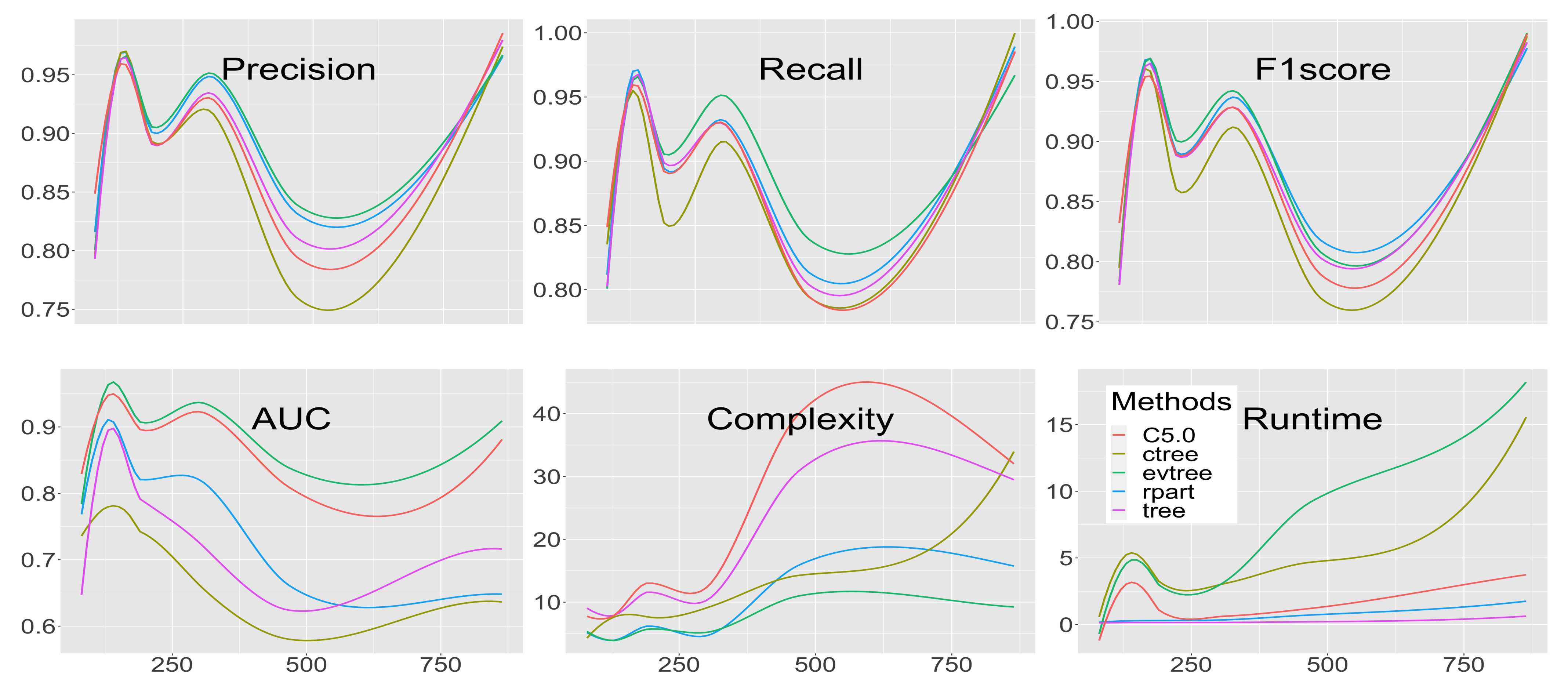
3. Results
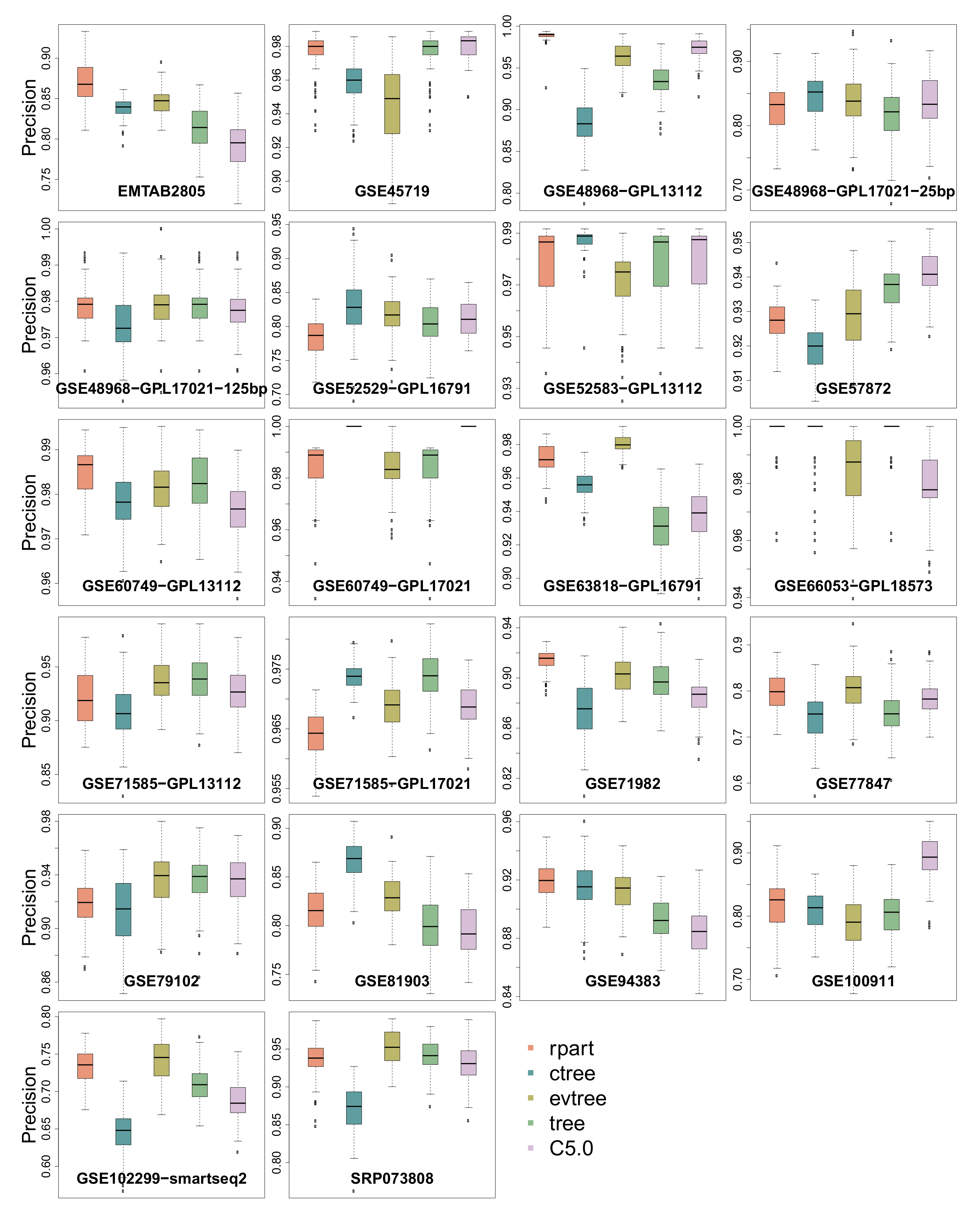
3.1. Precision
3.2. Recall
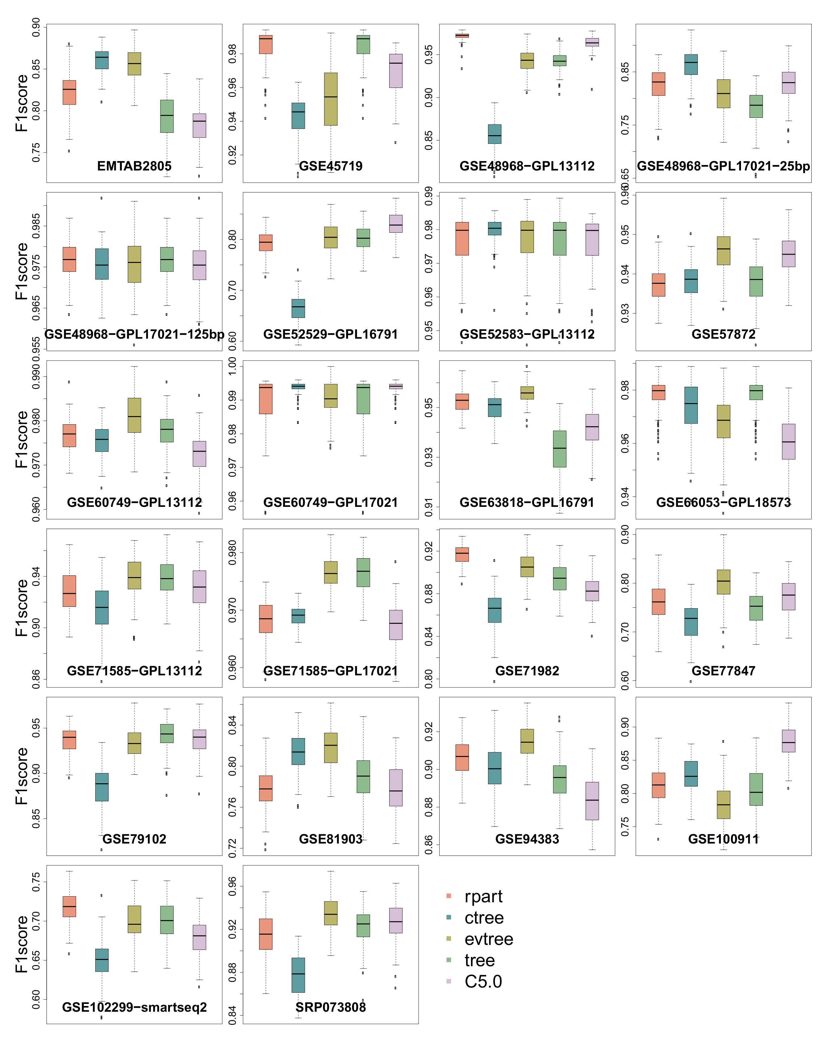
3.3. -Score
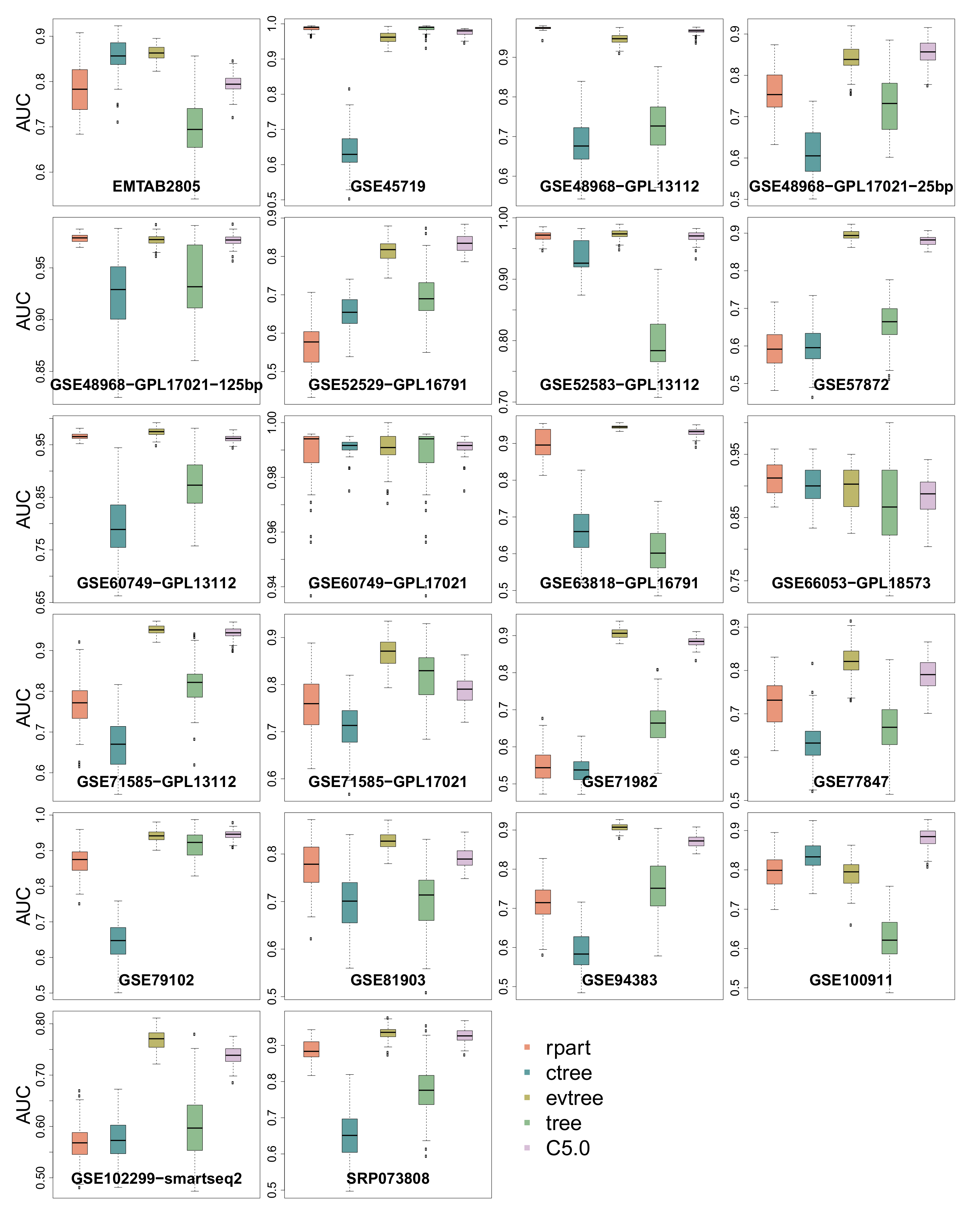
3.4. Area Under the Curve
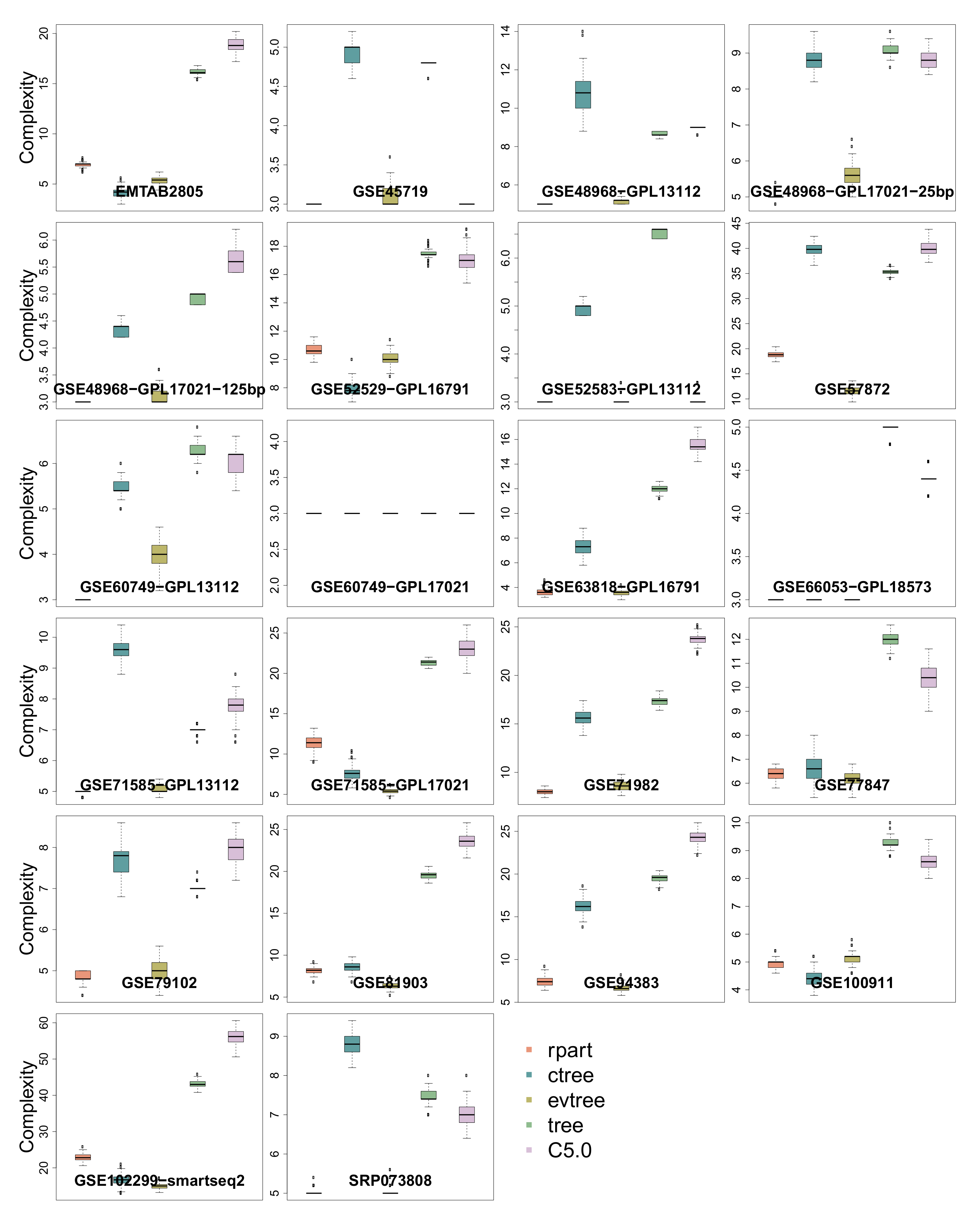
3.5. Complexity
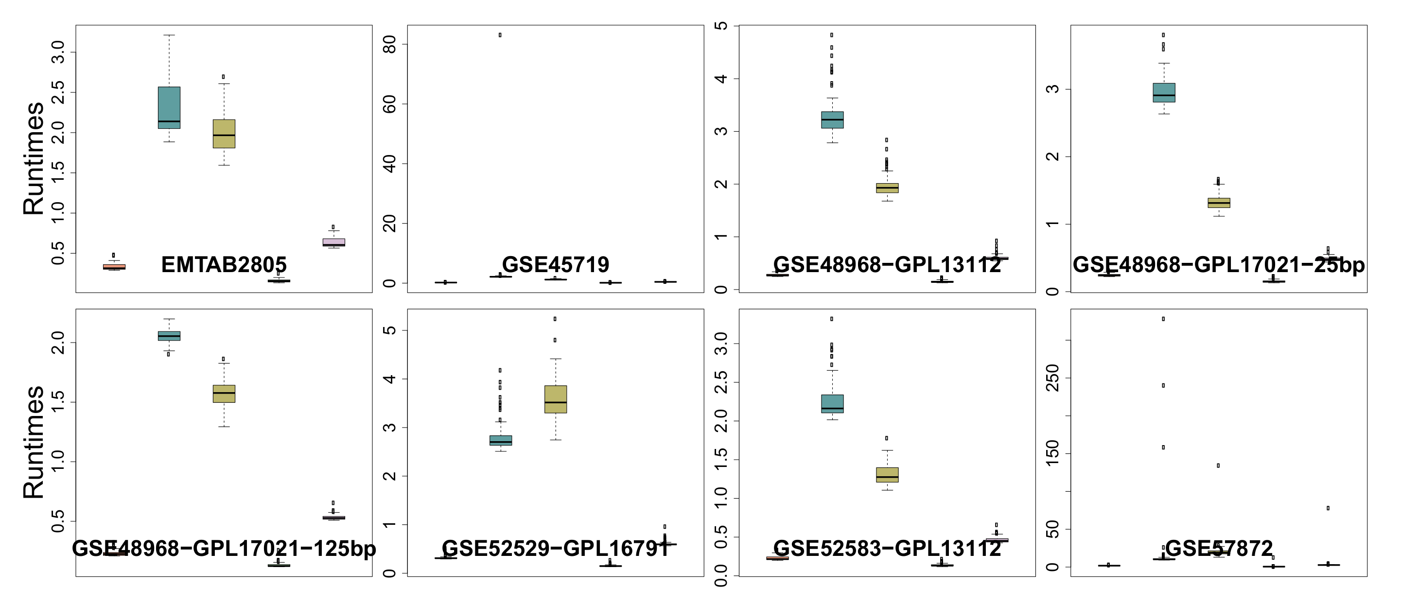
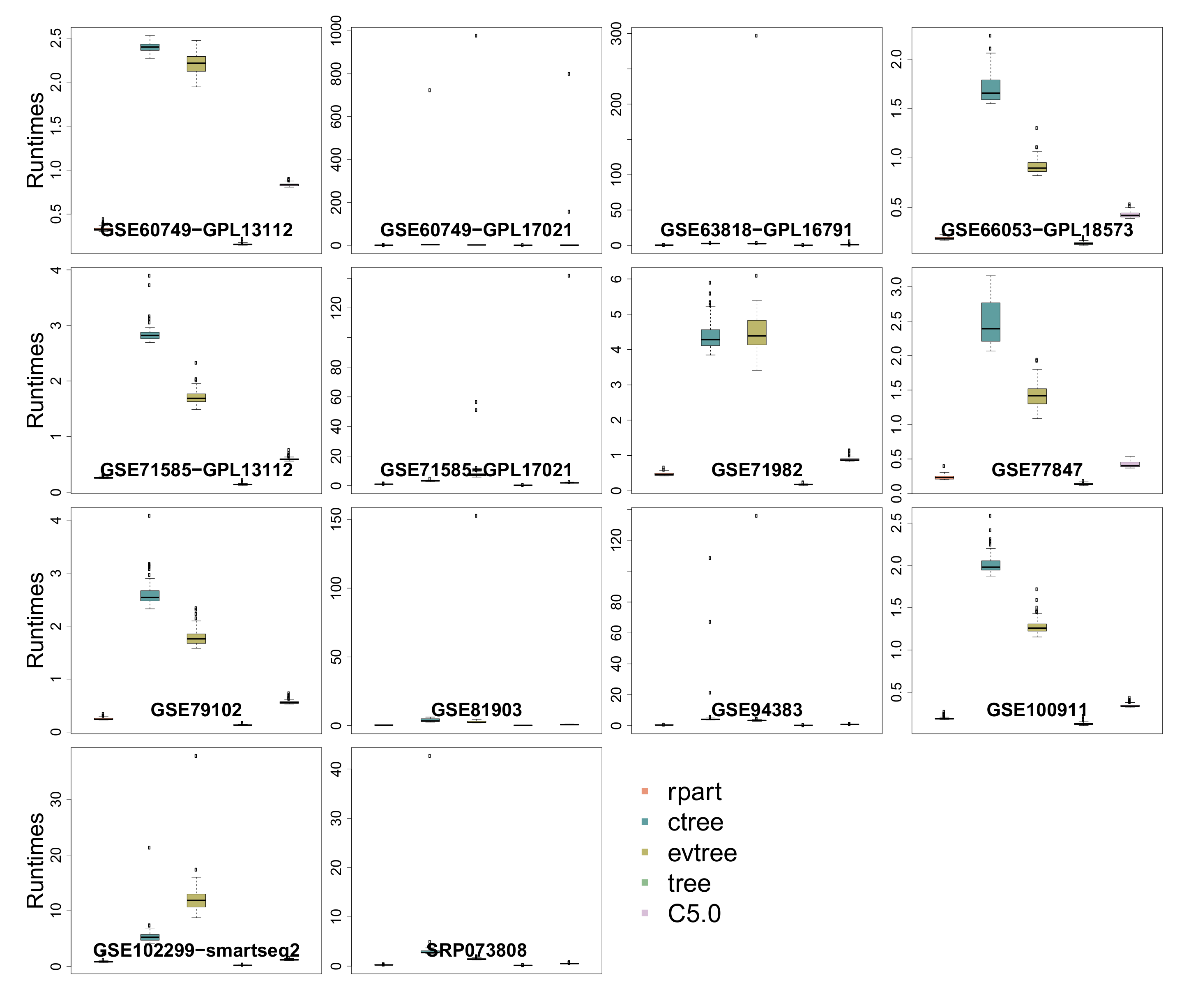
3.6. Runtime
4. Discussion and Conclusions
Supplementary Materials
Author Contributions
Funding
Data Availability Statement
Conflicts of Interest
Abbreviations
| AUC | Area Under the Curve |
| scRNA-seq | Single-cell Ribonucleicacid Sequencing |
| ROC | Receiver Operating Characteristic |
| TPM | Transcripts per million |
References
- Qian, J.; Olbrecht, S.; Boeckx, B.; Vos, H.; Laoui, D.; Etlioglu, E.; Wauters, E.; Pomella, V.; Verbandt, S.; Busschaert, P.; et al. A pan-cancer blueprint of the heterogeneous tumor microenvironment revealed by single-cell profiling. Cell Res. 2020, 30, 745–762. [Google Scholar] [CrossRef] [PubMed]
- Zhou, Y.; Yang, D.; Yang, Q.; Lv, X.; Huang, W.; Zhou, Z.; Wang, Y.; Zhang, Z.; Yuan, T.; Ding, X.; et al. Single-cell RNA landscape of intratumoral heterogeneity and immunosuppressive microenvironment in advanced osteosarcoma. Nat. Commun. 2020, 11, 6322. [Google Scholar] [CrossRef]
- Adams, T.S.; Schupp, J.C.; Poli, S.; Ayaub, E.A.; Neumark, N.; Ahangari, F.; Chu, S.G.; Raby, B.A.; DeIuliis, G.; Januszyk, M.; et al. Single-cell RNA-seq reveals ectopic and aberrant lung-resident cell populations in idiopathic pulmonary fibrosis. Sci. Adv. 2020, 6, eaba1983. [Google Scholar] [CrossRef] [PubMed]
- Seyednasrollah, F.; Rantanen, K.; Jaakkola, P.; Elo, L.L. ROTS: Reproducible RNA-seq biomarker detector—Prognostic markers for clear cell renal cell cancer. Nucleic Acids Res. 2015, 44, e1. [Google Scholar] [CrossRef] [PubMed]
- Arnold, C.D.; Gerlach, D.; Stelzer, C.; Boryń, Ł.M.; Rath, M.; Stark, A. Genome-Wide Quantitative Enhancer Activity Maps Identified by STARR-seq. Science 2013, 339, 1074–1077. [Google Scholar] [CrossRef]
- Nawy, T. Single-cell sequencing. Nat. Methods 2014, 11, 18. [Google Scholar] [CrossRef]
- Gawad, C.; Koh, W.; Quake, S.R. Single-cell genome sequencing: Current state of the science. Nat. Rev. Genet. 2016, 17, 175–188. [Google Scholar] [CrossRef]
- Metzker, M.L. Sequencing technologies—The next generation. Nat. Rev. Genet. 2010, 11, 31–46. [Google Scholar] [CrossRef]
- Elo, L.L.; Filen, S.; Lahesmaa, R.; Aittokallio, T. Reproducibility-Optimized Test Statistic for Ranking Genes in Microarray Studies. IEEE/ACM Trans. Comput. Biol. Bioinform. 2008, 5, 423–431. [Google Scholar] [CrossRef]
- Kowalczyk, M.S.; Tirosh, I.; Heckl, D.; Rao, T.N.; Dixit, A.; Haas, B.J.; Schneider, R.K.; Wagers, A.J.; Ebert, B.L.; Regev, A. Single-cell RNA-seq reveals changes in cell cycle and differentiation programs upon aging of hematopoietic stem cells. Genome Res. 2015, 25, 1860–1872. [Google Scholar] [CrossRef]
- Sandberg, R. Entering the era of single-cell transcriptomics in biology and medicine. Nat. Methods 2014, 11, 22–24. [Google Scholar] [CrossRef]
- Islam, S.; Kjällquist, U.; Moliner, A.; Zajac, P.; Fan, J.B.; Lönnerberg, P.; Linnarsson, S. Characterization of the single-cell transcriptional landscape by highly multiplex RNA-seq. Genome Res. 2011, 21, 1160–1167. [Google Scholar] [CrossRef]
- Patel, A.P.; Tirosh, I.; Trombetta, J.J.; Shalek, A.K.; Gillespie, S.M.; Wakimoto, H.; Cahill, D.P.; Nahed, B.V.; Curry, W.T.; Martuza, R.L.; et al. Single-cell RNA-seq highlights intratumoral heterogeneity in primary glioblastoma. Science 2014, 344, 1396–1401. [Google Scholar] [CrossRef]
- Habermann, A.C.; Gutierrez, A.J.; Bui, L.T.; Yahn, S.L.; Winters, N.I.; Calvi, C.L.; Peter, L.; Chung, M.I.; Taylor, C.J.; Jetter, C.; et al. Single-cell RNA sequencing reveals profibrotic roles of distinct epithelial and mesenchymal lineages in pulmonary fibrosis. Sci. Adv. 2020, 6, eaba1972. [Google Scholar] [CrossRef] [PubMed]
- Bauer, S.; Nolte, L.; Reyes, M. Segmentation of brain tumor images based on atlas-registration combined with a Markov-Random-Field lesion growth model. In Proceedings of the 2011 IEEE International Symposium on Biomedical Imaging: From Nano to Macro, Chicago, IL, USA, 30 March–2 April 2011; pp. 2018–2021. [Google Scholar] [CrossRef]
- Darmanis, S.; Sloan, S.A.; Zhang, Y.; Enge, M.; Caneda, C.; Shuer, L.M.; Hayden Gephart, M.G.; Barres, B.A.; Quake, S.R. A survey of human brain transcriptome diversity at the single cell level. Proc. Natl. Acad. Sci. USA 2015, 112, 7285–7290. [Google Scholar] [CrossRef] [PubMed]
- Pliner, H.A.; Shendure, J.; Trapnell, C. Supervised classification enables rapid annotation of cell atlases. Nat. Methods 2019, 16, 983–986. [Google Scholar] [CrossRef] [PubMed]
- Jaakkola, M.K.; Seyednasrollah, F.; Mehmood, A.; Elo, L.L. Comparison of methods to detect differentially expressed genes between single-cell populations. Briefings Bioinform. 2016, 18, 735–743. [Google Scholar] [CrossRef]
- Law, C.W.; Chen, Y.; Shi, W.; Smyth, G.K. Voom: Precision weights unlock linear model analysis tools for RNA-seq read counts. Genome Biol. 2014, 15, R29. [Google Scholar] [CrossRef]
- McCarthy, D.J.; Chen, Y.; Smyth, G.K. Differential expression analysis of multifactor RNA-Seq experiments with respect to biological variation. Nucleic Acids Res. 2012, 40, 4288–4297. [Google Scholar] [CrossRef]
- Rapaport, F.; Khanin, R.; Liang, Y.; Pirun, M.; Krek, A.; Zumbo, P.; Mason, C.E.; Socci, N.D.; Betel, D. Comprehensive evaluation of differential gene expression analysis methods for RNA-seq data. Genome Biol. 2013, 14, 3158. [Google Scholar] [CrossRef]
- Miao, Z.; Zhang, X. Differential expression analyses for single-cell RNA-Seq: Old questions on new data. Quant. Biol. 2016, 4, 243–260. [Google Scholar] [CrossRef]
- Stegle, O.; Teichmann, S.A.; Marioni, J.C. Computational and analytical challenges in single-cell transcriptomics. Nat. Rev. Genet. 2015, 16, 133–145. [Google Scholar] [CrossRef] [PubMed]
- Oshlack, A.; Robinson, M.D.; Young, M.D. From RNA-seq reads to differential expression results. Genome Biol. 2010, 11, 220. [Google Scholar] [CrossRef] [PubMed]
- Seyednasrollah, F.; Laiho, A.; Elo, L.L. Comparison of software packages for detecting differential expression in RNA-seq studies. Briefings Bioinform. 2013, 16, 59–70. [Google Scholar] [CrossRef]
- Wang, T.; Li, B.; Nelson, C.E.; Nabavi, S. Comparative analysis of differential gene expression analysis tools for single-cell RNA sequencing data. BMC Bioinform. 2019, 20, 40. [Google Scholar] [CrossRef]
- Krzak, M.; Raykov, Y.; Boukouvalas, A.; Cutillo, L.; Angelini, C. Benchmark and Parameter Sensitivity Analysis of Single-Cell RNA Sequencing Clustering Methods. Front. Genet. 2019, 10, 1253. [Google Scholar] [CrossRef]
- Anders, S.; Pyl, P.T.; Huber, W. HTSeq—A Python framework to work with high-throughput sequencing data. Bioinformatics 2014, 31, 166–169. [Google Scholar] [CrossRef]
- Li, S.; Łabaj, P.; Zumbo, P.; Sykacek, P.; Shi, W.; Shi, L.; Phan, J.; Wu, P.Y.; Wang, M.; Wang, C.; et al. Detecting and correcting systematic variation in large-scale RNA sequencing data. Nat. Biotechnol. 2014, 32, 888–895. [Google Scholar] [CrossRef]
- Delmans, M.; Hemberg, M. Discrete distributional differential expression (D 3 E)—A tool for gene expression analysis of single-cell RNA-seq data. BMC Bioinform. 2016, 17, 110. [Google Scholar] [CrossRef]
- Soneson, C.; Robinson, M.D. Bias, robustness and scalability in single-cell differential expression analysis. Nat. Methods 2018, 15, 255–261. [Google Scholar] [CrossRef]
- Breiman, L.; Friedman, J.H.; Olshen, R.A.; Stone, C.J. Classification and Regression Trees; The Wadsworth & Brooks/Cole statistics/probability Series; Wadsworth & Brooks/Cole Advanced Books & Software: Monterey, CA, USA, 1984. [Google Scholar]
- Hothorn, T.; Hornik, K.; Zeileis, A. Unbiased Recursive Partitioning: A Conditional Inference Framework. J. Comput. Graph. Stat. 2006, 15, 651–674. [Google Scholar] [CrossRef]
- Grubinger, T.; Zeileis, A.; Pfeiffer, K.P. evtree: Evolutionary Learning of Globally Optimal Classification and Regression Trees in R. J. Stat. Softw. Artic. 2014, 61, 1–29. [Google Scholar] [CrossRef]


| Data Set | ID | Organism | Brief Description | # of Cells | Protocol |
|---|---|---|---|---|---|
| EMTAB2805 | Buettner2015 | Mus musculus | mESC in different cell cycle stages | 288 | SMARTer C1 |
| GSE100911 | Tang2017 | Danio rerio | hematopoietic and renal cell heterogeneity | 245 | Smart-Seq2 |
| GSE102299- smartseq2 | Wallrapp2017 | Mus musculus | innate lymphoid cells from mouse lungs after various treatments | 752 | Smart-Seq2 |
| GSE45719 | Deng2014 | Mus musculus | development from zygote to blastocyst + adult liver | 291 | SMART-Seq |
| GSE48968- GPL13112 | Shalek2014 | Mus musculus | dendritic cells stimulated with pathogenic components | 1378 | SMARTer C1 |
| GSE48968- GPL17021- 125bp | Shalek2014 | Mus musculus | dendritic cells stimulated with pathogenic components | 935 | SMARTer C1 |
| GSE48968- GPL17021- 25bp | Shalek2014 | Mus musculus | dendritic cells stimulated with pathogenic components | 99 | SMARTer C1 |
| GSE52529- GPL16791 | Trapnell2014 | Homo sapiens | primary myoblasts over a time course of serum-induced differentiation | 288 | SMARTer C1 |
| GSE52583- GPL13112 | Treutlein2014 | Mus musculus | lung epithelial cells at different developmental stages | 171 | SMARTer C1 |
| GSE57872 | Patel2014 | Homo sapiens | glioblastoma cells from tumors + gliomasphere cell lines | 864 | SMART-Seq |
| GSE60749- GPL13112 | Kumar2014 | Mus musculus | mESCs with various genetic perturbations, cultured in different media | 268 | SMARTer C1 |
| GSE60749- GPL17021 | Kumar2014 | Mus musculus | mESCs with various genetic perturbations, cultured in different media | 147 | SMARTer C1 |
| GSE63818- GPL16791 | Guo2015 | Homo sapiens | primordial germ cells from embryos at different times of gestation | 328 | Tang |
| GSE66053- GPL18573 | Padovan Merhar2015 | Homo sapiens | live and fixed single cells | 96 | Fluidigm C1 Auto prep |
| GSE71585- GPL13112 | Tasic2016 | Mus musculus | cell type identification in primary visual cortex | 1035 | SMARTer |
| GSE71585- GPL17021 | Tasic2016 | Mus musculus | cell type identification in primary visual cortex | 749 | SMARTer |
| GSE71982 | Burns2015 | Mus musculus | utricular and cochlear sensory epithelia of newborn mice | 313 | SMARTer C1 |
| GSE77847 | Meyer2016 | Mus musculus | Dnmt3a loss of function in Flt3-ITD and Dnmt3a-mutant AML | 96 | SMARTer C1 |
| GSE79102 | Kiselev2017 | Homo sapiens | different patients with myeloproloferative disease | 181 | Smart-Seq2 |
| GSE81903 | Shekhar2016 | Mus musculus | P17 retinal cells from the Kcng4-cre;stop-YFP X Thy1-stop-YFP Line#1 mice | 384 | Smart-Seq2 |
| SRP073808 | Koh2016 | Homo sapiens | in vitro cultured H7 embryonic stem cells (WiCell) and H7-derived downstream early mesoderm progenitors | 651 | SMARTer C1 |
| GSE94383 | Lane2017 | Mus musculus | LPS stimulated and unstimulated 264.7 cells | 839 | Smart-Seq2 |
| # | Data Set | Phenotype | # of 1 s | # of 0 s |
|---|---|---|---|---|
| 1 | EMTAB2805 | Cell Stages (G1 & G2M) | 96 | 96 |
| 2 | GSE100911 | 16-cell stage blastomere & Mid blastocyst cell (92–94 h post-fertilization) | 43 | 38 |
| 3 | GSE102299-smartseq2 | treatment: IL25 & treatment: IL33 | 188 | 282 |
| 4 | GSE45719 | 16-cell stage blastomere & Mid blastocyst cell (92–94 h post-fertilization) | 50 | 60 |
| 5 | GSE48968-GPL13112 | BMDC (Unstimulated Replicate Experiment) & BMDC (1 h LPS Stimulation) | 96 | 95 |
| 6 | GSE48968-GPL17021-125bp | BMDC (On Chip 4 h LPS Stimulation) & BMDC (2 h IFN-B Stimulation) | 90 | 94 |
| 7 | GSE48968-GPL17021-25bp | LPS4h, GolgiPlug 1 h & stimulation: LPS4h, GolgiPlug 2 h | 46 | 53 |
| 8 | GSE52529-GPL16791 | hour post serum-switch: 0 & hour post serum-switch: 24 | 96 | 96 |
| 9 | GSE52583-GPL13112 | age: Embryonic day 18.5 & age: Embryonic day 14.5 | 80 | 45 |
| 10 | GSE57872 | cell type: Glioblastoma & cell type: Gliomasphere Cell Line | 672 | 192 |
| 11 | GSE60749-GPL13112 | culture conditions: serum+LIF & culture conditions: 2i+LIF | 174 | 94 |
| 12 | GSE60749-GPL17021 | serum+LIF & Selection in ITSFn, followed by expansion in N2+bFGF/laminin | 93 | 54 |
| 13 | GSE63818-GPL16791 | male & female | 197 | 131 |
| 14 | GSE66053-GPL18573 | Cells were added to the Fluidigm C1 ... & Fixed cells were added to the Fluidigm C1 ... | 82 | 14 |
| 15 | GSE71585-GPL13112 | input material: single cell & tdtomato labelling: positive (partially) | 81 | 108 |
| 16 | GSE71585-GPL17021 | dissection: All & input material: single cell | 691 | 57 |
| 17 | GSE71982 | Vestibular epithelium & Cochlear epithelium | 160 | 153 |
| 18 | GSE77847 | sample type: cKit+ Flt3ITD/ITD,Dnmt3afl/- MxCre AML-1 & sample type: cKit+ Flt3ITD/ITD,Dnmt3afl/- MxCre AML-2 | 48 | 48 |
| 19 | GSE79102 | patient 1 scRNA-seq & patient 2 scRNA-seq | 85 | 96 |
| 20 | GSE81903 | retina id: 1Ra & retina id: 1la | 96 | 96 |
| 21 | SRP073808 | H7hESC & H7_derived_APS | 77 | 64 |
| 22 | GSE94383 | time point: 0 & min time point: 75 min | 186 | 145 |
| platform | ×86_64-apple-darwin15.6.0 | |
| arch | ×86_64 | |
| os | darwin15.6.0 | |
| system | ×86_64, darwin15.6.0 | |
| status | ||
| major | 3 | |
| minor | 6.1 | |
| year | 2019 | |
| month | 07 | |
| day | 05 | |
| svn rev | 76782 | |
| language | R | |
| version.string | R version 3.6.1 (05-07-2019) | |
| nickname | Action of the Toes |
| rpart | ctree | evtree | tree | C5.0 | |
|---|---|---|---|---|---|
| Precision | 9 | 8 | 9 | 8 | 8 |
| Recall | 8 | 4 | 10 | 8 | 7 |
| score | 11 | 6 | 13 | 9 | 7 |
| AUC | 7 | 2 | 16 | 2 | 9 |
| Complexity | 1 | 5 | 1 | 8 | 11 |
| Runtime | 0 | 0 | 0 | 22 | 0 |
Publisher’s Note: MDPI stays neutral with regard to jurisdictional claims in published maps and institutional affiliations. |
© 2021 by the authors. Licensee MDPI, Basel, Switzerland. This article is an open access article distributed under the terms and conditions of the Creative Commons Attribution (CC BY) license (https://creativecommons.org/licenses/by/4.0/).
Share and Cite
Alaqeeli, O.; Xing, L.; Zhang, X. Software Benchmark—Classification Tree Algorithms for Cell Atlases Annotation Using Single-Cell RNA-Sequencing Data. Microbiol. Res. 2021, 12, 317-334. https://doi.org/10.3390/microbiolres12020022
Alaqeeli O, Xing L, Zhang X. Software Benchmark—Classification Tree Algorithms for Cell Atlases Annotation Using Single-Cell RNA-Sequencing Data. Microbiology Research. 2021; 12(2):317-334. https://doi.org/10.3390/microbiolres12020022
Chicago/Turabian StyleAlaqeeli, Omar, Li Xing, and Xuekui Zhang. 2021. "Software Benchmark—Classification Tree Algorithms for Cell Atlases Annotation Using Single-Cell RNA-Sequencing Data" Microbiology Research 12, no. 2: 317-334. https://doi.org/10.3390/microbiolres12020022
APA StyleAlaqeeli, O., Xing, L., & Zhang, X. (2021). Software Benchmark—Classification Tree Algorithms for Cell Atlases Annotation Using Single-Cell RNA-Sequencing Data. Microbiology Research, 12(2), 317-334. https://doi.org/10.3390/microbiolres12020022