

A Multimodal Multi-Stage Deep Learning Model for the Diagnosis of Alzheimer’s Disease Using EEG Measurements


Abstract
1. Introduction
2. Data Acquisition
2.1. Participants
2.2. EEG Recordings
3. Methodology
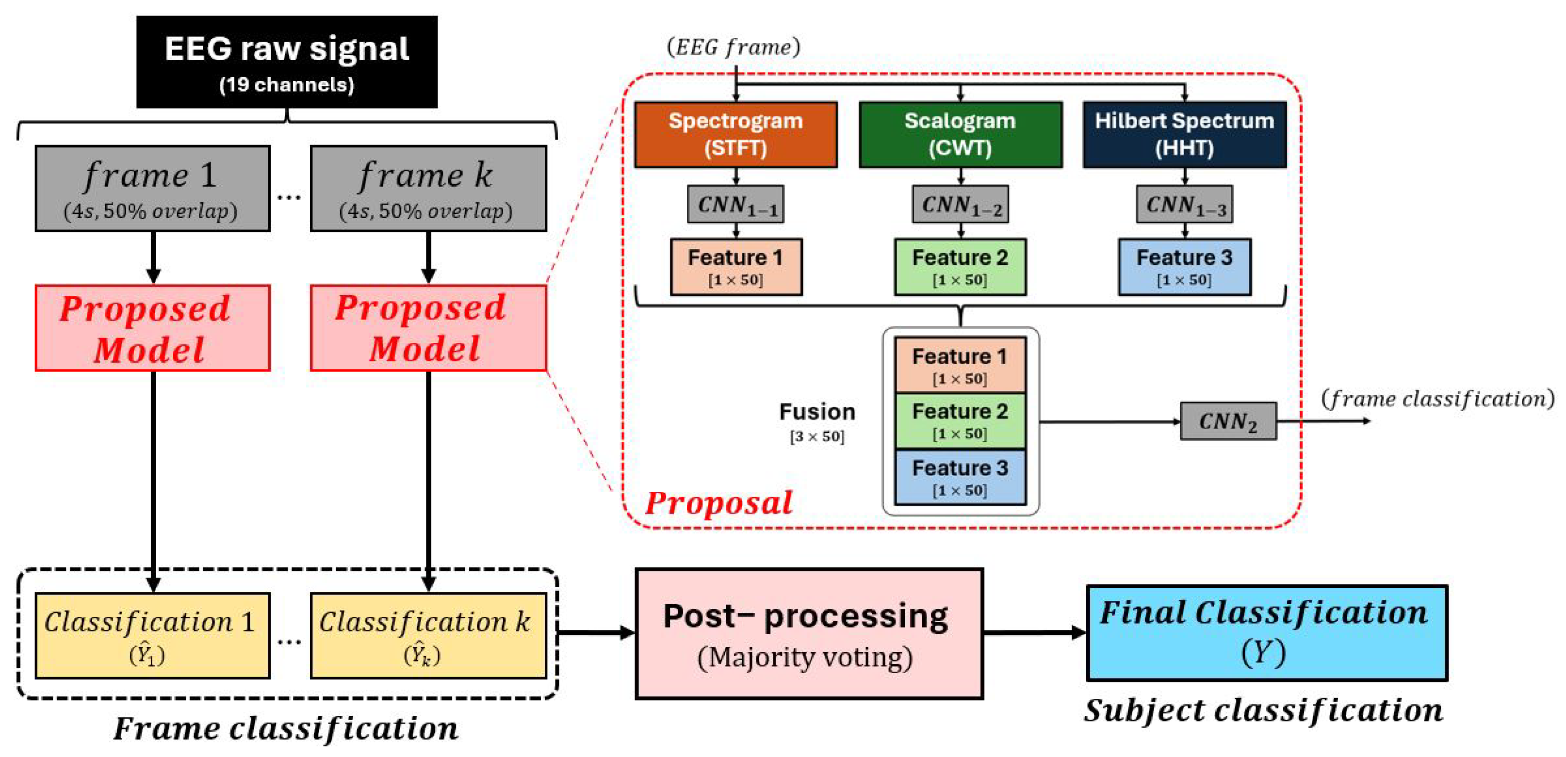
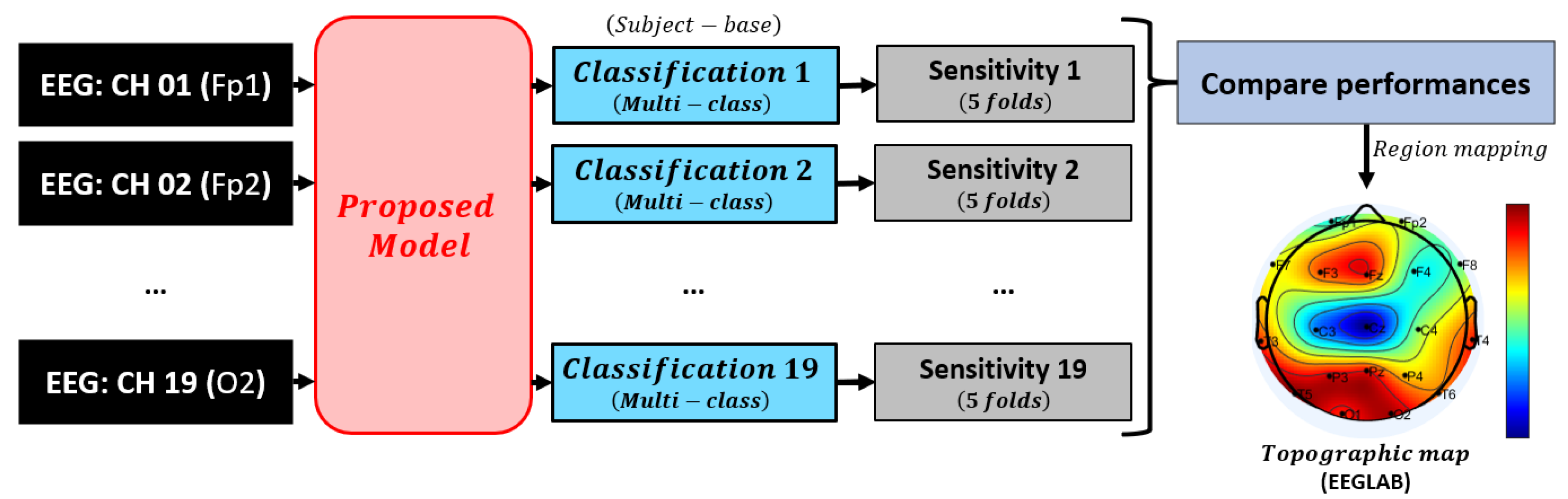
3.1. Model Overview
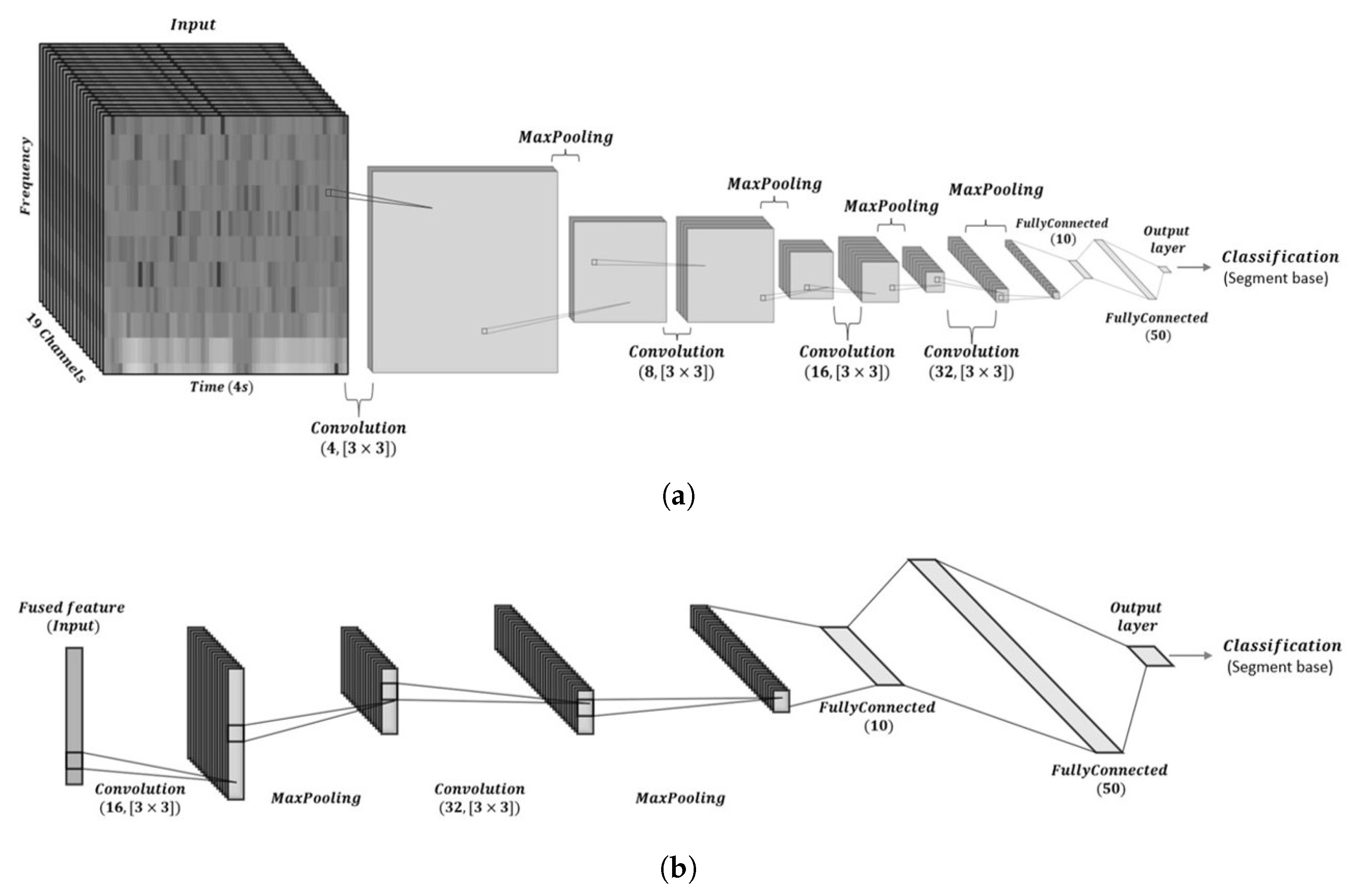
3.2. CNN Architecture Design and Training Parameters
3.2.1. Architecture Rationale
3.2.2. Training Parameters and Optimization
3.3. Data Analysis
3.3.1. Spectrogram
3.3.2. Scalogram
3.3.3. Hilbert Spectrum
3.4. Convolutional Layer
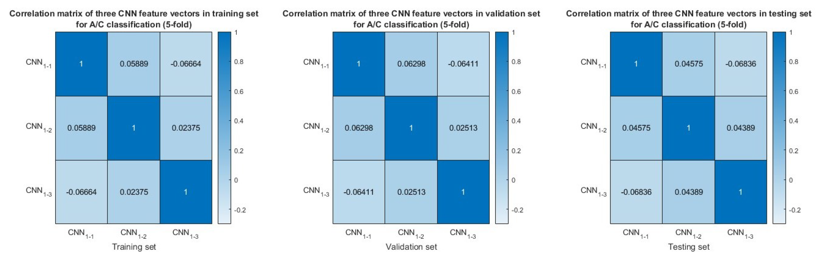
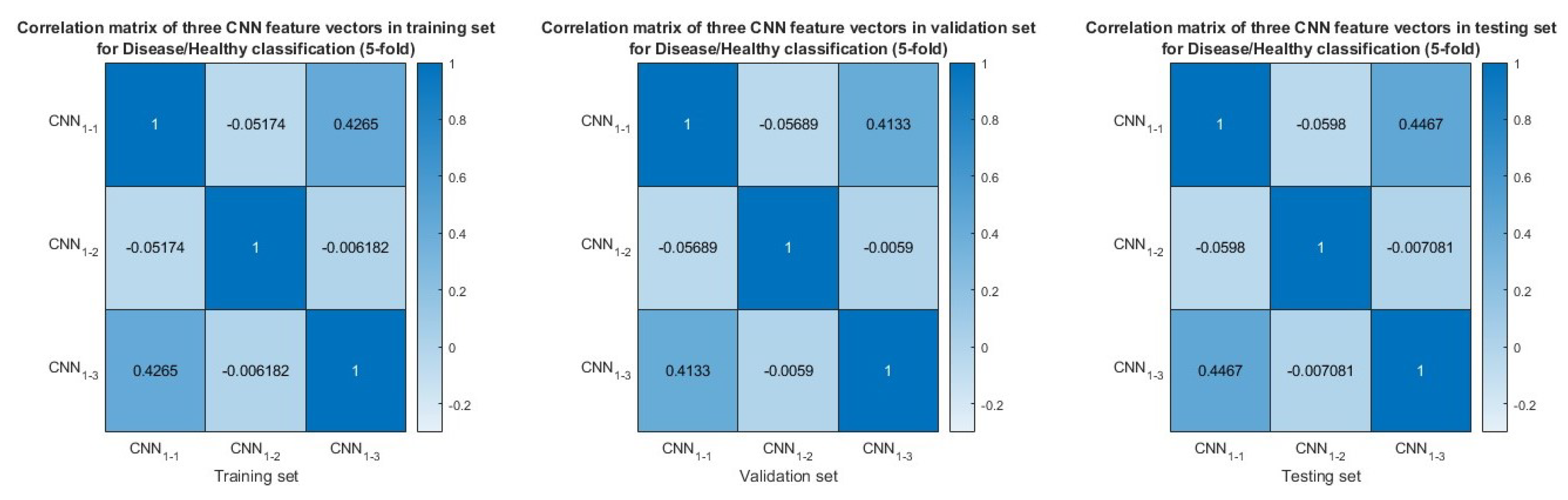
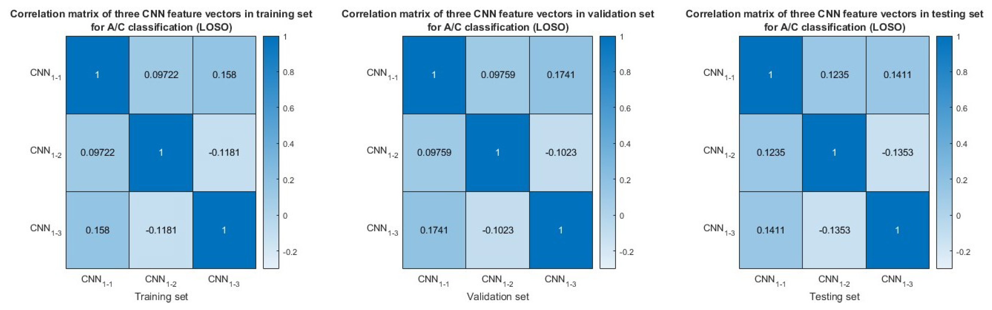
3.5. Feature Similarity Analysis
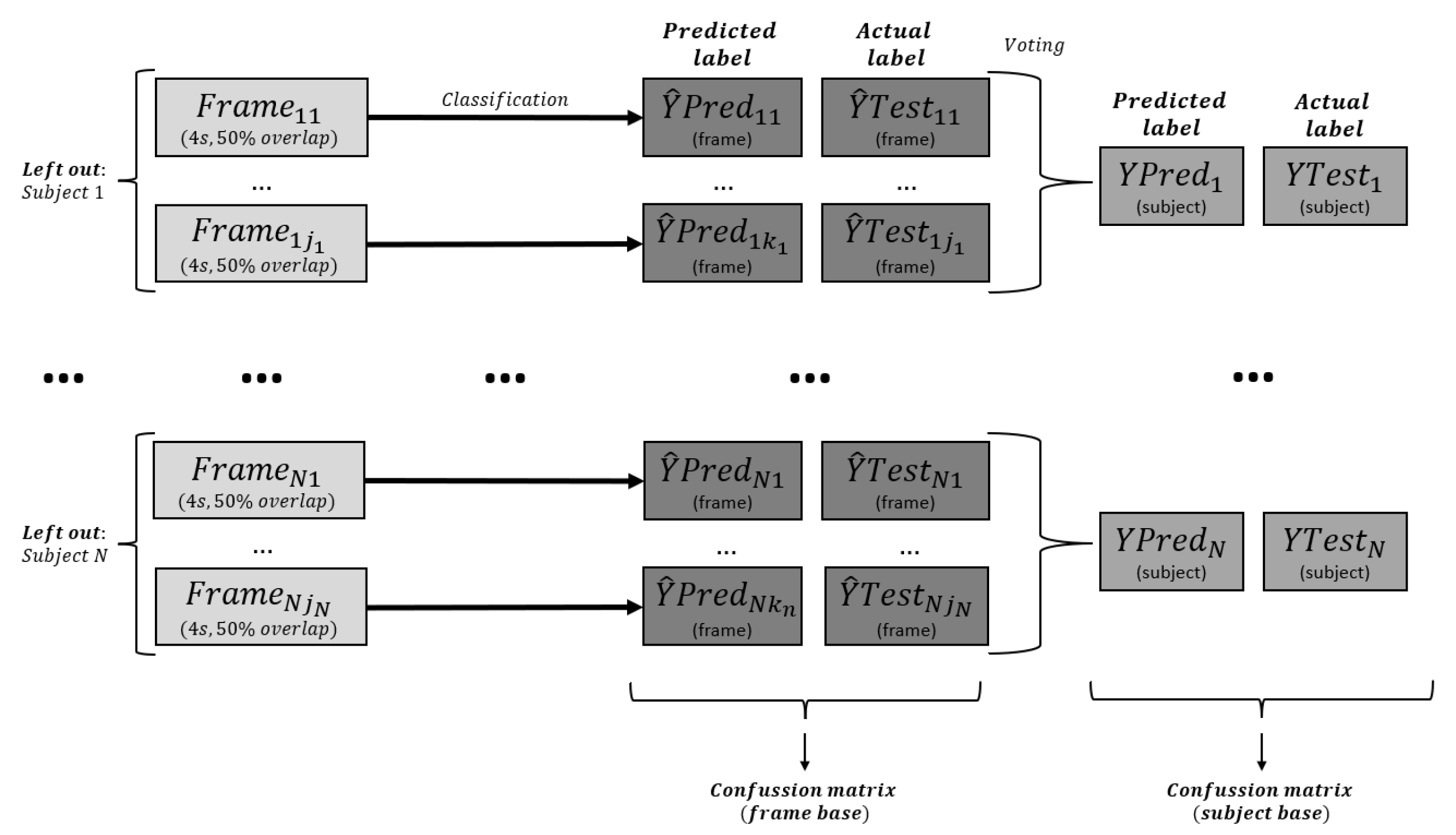
3.6. Post-Processing
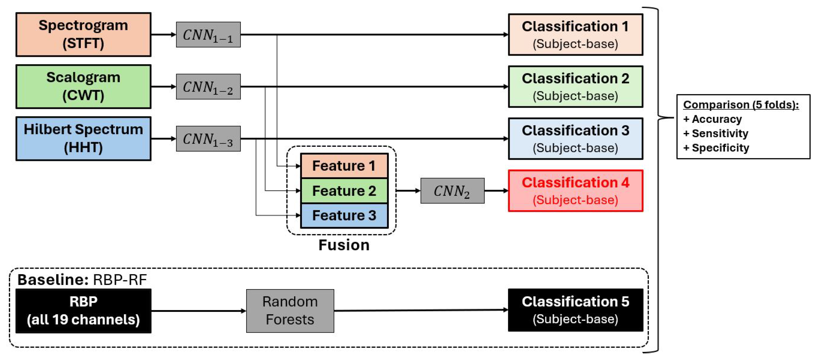
3.7. Model Evaluation
3.7.1. Statistical Analysis and Significance Testing
3.7.2. Statistical Significance Analysis of Feature Extraction Methods
3.7.3. Confidence Intervals and Error Reporting
4. Results
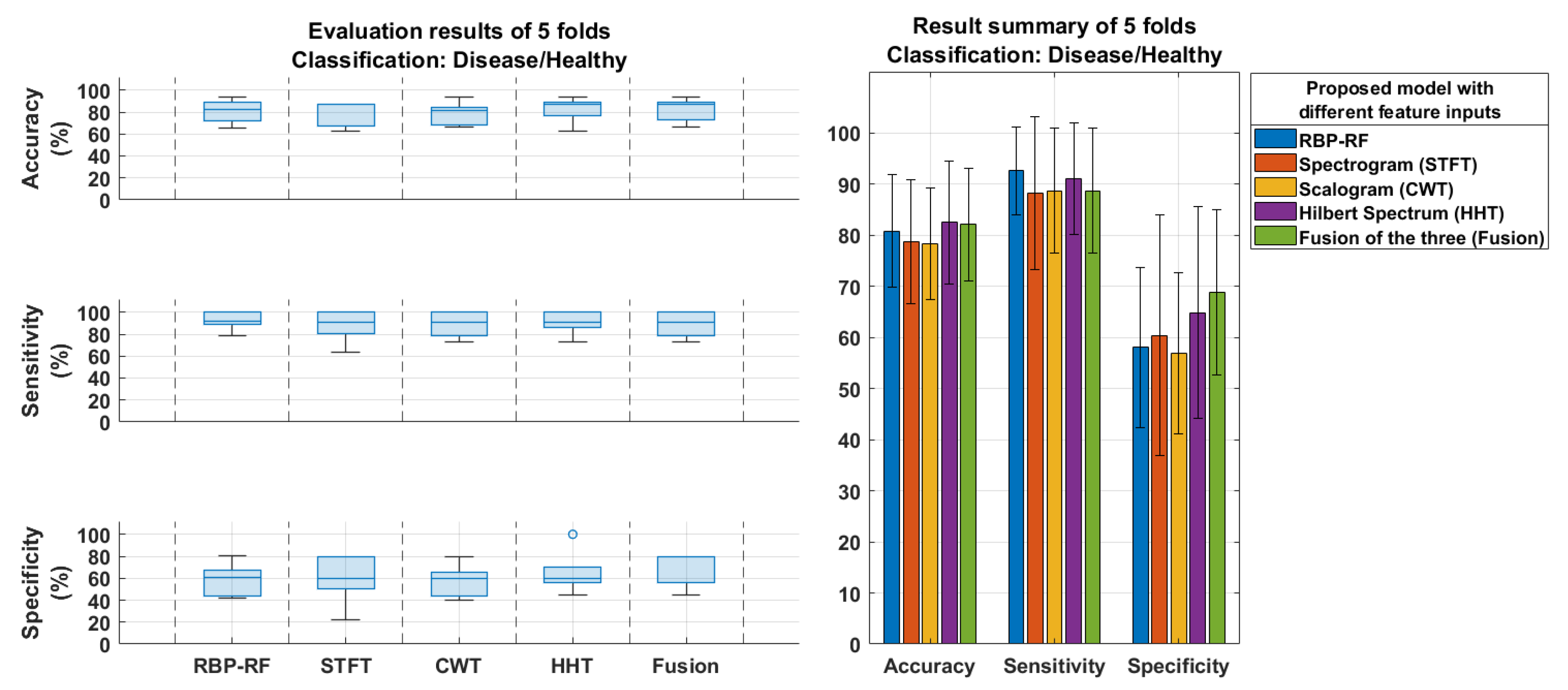
4.1. Model Classification Results
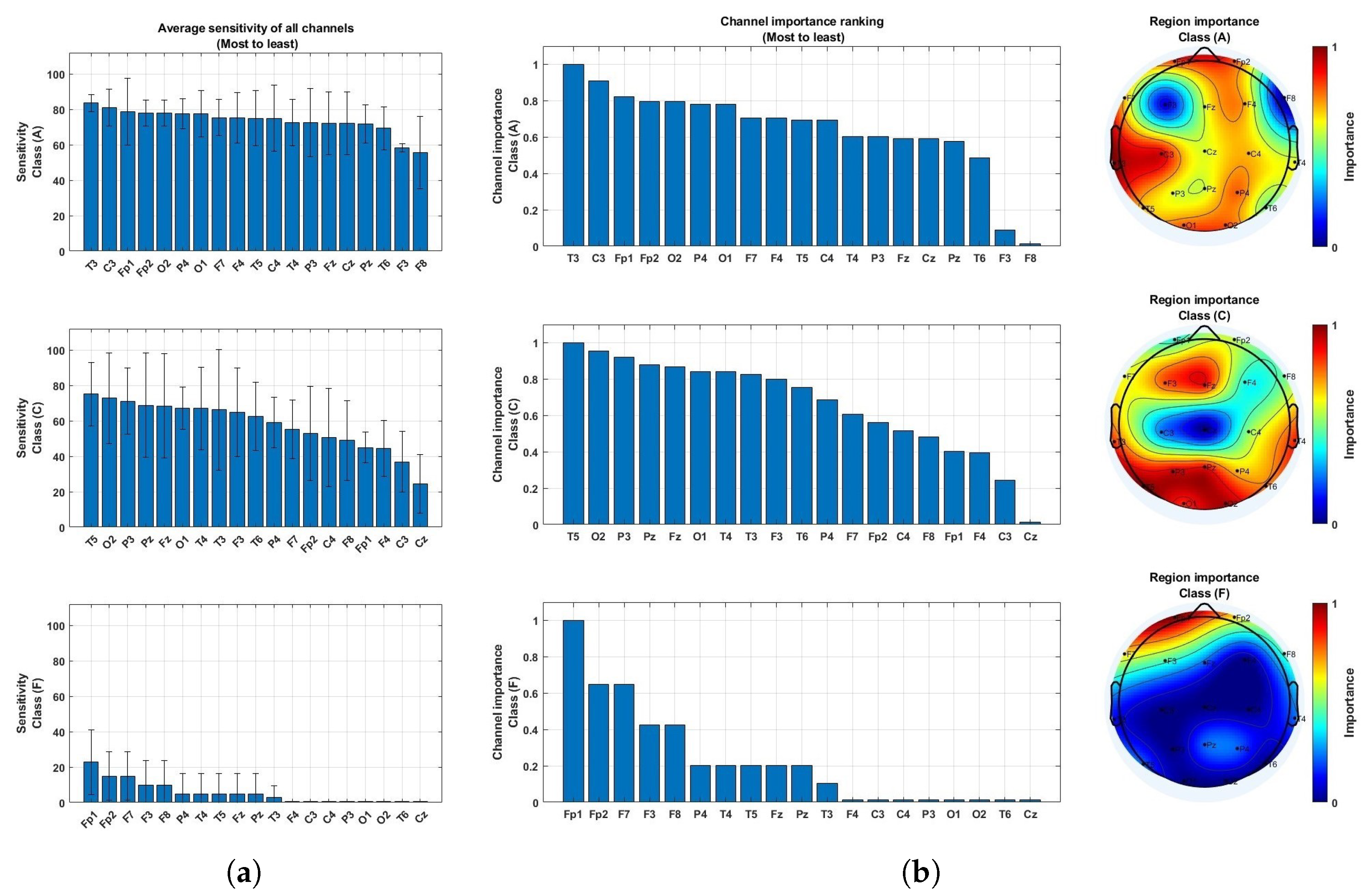
4.2. Brain Region Importance
4.3. Comparison to Prior Studies
5. Discussion
6. Conclusions
Author Contributions
Funding
Institutional Review Board Statement
Informed Consent Statement
Data Availability Statement
Conflicts of Interest
References
- Chowdhary, N.; Barbui, C.; Anstey, K.J.; Kivipelto, M.; Barbera, M.; Peters, R.; Zheng, L.; Kulmala, J.; Stephen, R.; Ferri, C.P.; et al. Reducing the risk of cognitive decline and dementia: WHO recommendations. Front. Neurol. 2022, 12, 765584. [Google Scholar] [CrossRef]
- Kirshner, H.S. Frontotemporal dementia and primary progressive aphasia, a review. Neuropsychiatr. Dis. Treat. 2014, 10, 1045–1055. [Google Scholar] [CrossRef] [PubMed]
- Ma, D.; Lu, D.; Popuri, K.; Wang, L.; Beg, M.F.; Initiative, A.D.N. Differential diagnosis of frontotemporal dementia, alzheimer’s disease, and normal aging using a multi-scale multi-type feature generative adversarial deep neural network on structural magnetic resonance images. Front. Neurosci. 2020, 14, 853. [Google Scholar] [CrossRef] [PubMed]
- Xu, X.; Lin, L.; Sun, S.; Wu, S. A review of the application of three-dimensional convolutional neural networks for the diagnosis of Alzheimer’s disease using neuroimaging. Rev. Neurosci. 2023, 34, 649–670. [Google Scholar] [CrossRef] [PubMed]
- Hort, J.; O’brien, J.; Gainotti, G.; Pirttila, T.; Popescu, B.; Rektorová, I.; Sorbi, S.; Scheltens, P.; on behalf of the EFNS Scientist Panel on Dementia. EFNS guidelines for the diagnosis and management of Alzheimer’s disease. Eur. J. Neurol. 2010, 17, 1236–1248. [Google Scholar] [CrossRef]
- Güntekin, B.; Erdal, F.; Bölükbaş, B.; Hanoğlu, L.; Yener, G.; Duygun, R. Alterations of resting-state Gamma frequency characteristics in aging and Alzheimer’s disease. Cogn. Neurodynamics 2023, 17, 829–844. [Google Scholar] [CrossRef]
- Göker, H. Welch Spectral Analysis and Deep Learning Approach for Diagnosing Alzheimer’s Disease from Resting-State EEG Recordings. Trait. Signal 2023, 40, 257–264. [Google Scholar] [CrossRef]
- Şeker, M.; Özerdem, M.S. Automated Detection of Alzheimer’s Disease using raw EEG time series via. DWT-CNN model. Dicle Üniversitesi Mühendislik Fakültesi Mühendislik Derg. 2023, 13, 673–684. [Google Scholar] [CrossRef]
- Sridhar, S.; Romney, A.; Manian, V. A Deep Neural Network for Working Memory Load Prediction from EEG Ensemble Empirical Mode Decomposition. Information 2023, 14, 473. [Google Scholar] [CrossRef]
- Song, Z.; Deng, B.; Wang, J.; Yi, G. An EEG-based systematic explainable detection framework for probing and localizing abnormal patterns in Alzheimer’s disease. J. Neural Eng. 2022, 19, 036007. [Google Scholar] [CrossRef]
- Chaddad, A.; Wu, Y.; Kateb, R.; Bouridane, A. Electroencephalography signal processing: A comprehensive review and analysis of methods and techniques. Sensors 2023, 23, 6434. [Google Scholar] [CrossRef]
- Rutkowski, T.M.; Abe, M.S.; Komendzinski, T.; Sugimoto, H.; Narebski, S.; Otake-Matsuura, M. Machine learning approach for early onset dementia neurobiomarker using EEG network topology features. Front. Hum. Neurosci. 2023, 17, 1155194. [Google Scholar] [CrossRef]
- Kim, N.H.; Yang, D.W.; Choi, S.H.; Kang, S.W. Machine learning to predict brain amyloid pathology in pre-dementia Alzheimer’s disease using QEEG features and genetic algorithm heuristic. Front. Comput. Neurosci. 2021, 15, 755499. [Google Scholar] [CrossRef]
- Aljalal, M.; Molinas, M.; Aldosari, S.A.; AlSharabi, K.; Abdurraqeeb, A.M.; Alturki, F.A. Mild cognitive impairment detection with optimally selected EEG channels based on variational mode decomposition and supervised machine learning. Biomed. Signal Process. Control 2024, 87, 105462. [Google Scholar] [CrossRef]
- Perez-Valero, E.; Morillas, C.; Lopez-Gordo, M.A.; Minguillon, J. Supporting the Detection of Early Alzheimer’s Disease with a Four-Channel EEG Analysis. Int. J. Neural Syst. 2023, 33, 2350021. [Google Scholar] [CrossRef] [PubMed]
- Hadiyoso, S.; Wijayanto, I.; Humairani, A. Entropy and Fractal Analysis of EEG Signals for Early Detection of Alzheimer’s Dementia. Trait. Signal 2023, 40, 1673–1679. [Google Scholar] [CrossRef]
- Javaid, H.; Manor, R.; Kumarnsit, E.; Chatpun, S. Decision tree in working memory task effectively characterizes EEG signals in healthy aging adults. IRBM 2022, 43, 705–714. [Google Scholar] [CrossRef]
- Dauwan, M.; Linszen, M.M.; Lemstra, A.W.; Scheltens, P.; Stam, C.J.; Sommer, I.E. EEG-based neurophysiological indicators of hallucinations in Alzheimer’s disease: Comparison with dementia with Lewy bodies. Neurobiol. Aging 2018, 67, 75–83. [Google Scholar] [CrossRef]
- Li, K.; Wang, J.; Li, S.; Yu, H.; Zhu, L.; Liu, J.; Wu, L. Feature extraction and identification of Alzheimer’s disease based on latent factor of multi-channel EEG. IEEE Trans. Neural Syst. Rehabil. Eng. 2021, 29, 1557–1567. [Google Scholar] [CrossRef]
- Yang, S.; Bornot, J.M.S.; Wong-Lin, K.; Prasad, G. M/EEG-based bio-markers to predict the MCI and Alzheimer’s disease: A review from the ML perspective. IEEE Trans. Biomed. Eng. 2019, 66, 2924–2935. [Google Scholar] [CrossRef]
- Xia, W.; Zhang, R.; Zhang, X.; Usman, M. A novel method for diagnosing Alzheimer’s disease using deep pyramid CNN based on EEG signals. Heliyon 2023, 9, e14858. [Google Scholar] [CrossRef] [PubMed]
- Salah, F.; Guesmi, D.; Ayed, Y.B. A Convolutional Recurrent Neural Network Model for Classification of Parkinson’s Disease from Resting State Multi-channel EEG Signals. In Proceedings of the International Conference on Computational Collective Intelligence, Leipzig, Germany, 9–11 September 2023; Springer: Berlin/Heidelberg, Germany, 2023; pp. 136–146. [Google Scholar]
- Alessandrini, M.; Biagetti, G.; Crippa, P.; Falaschetti, L.; Luzzi, S.; Turchetti, C. EEG-Based Neurodegenerative Disease Classification using LSTM Neural Networks. In Proceedings of the 2023 IEEE Statistical Signal Processing Workshop (SSP), Hanoi, Vietnam, 2–5 July 2023; IEEE: Piscataway, NJ, USA, 2023; pp. 428–432. [Google Scholar]
- Shen, X.; Lin, L.; Xu, X.; Wu, S. Effects of Patchwise Sampling Strategy to Three-Dimensional Convolutional Neural Network-Based Alzheimer’s Disease Classification. Brain Sci. 2023, 13, 254. [Google Scholar] [CrossRef]
- Saraceno, C.; Cervellati, C.; Trentini, A.; Crescenti, D.; Longobardi, A.; Geviti, A.; Bonfiglio, N.S.; Bellini, S.; Nicsanu, R.; Fostinelli, S.; et al. Serum Beta-Secretase 1 Activity Is a Potential Marker for the Differential Diagnosis between Alzheimer’s Disease and Frontotemporal Dementia: A Pilot Study. Int. J. Mol. Sci. 2024, 25, 8354. [Google Scholar] [CrossRef]
- Abdelwahab, M.M.; Al-Karawi, K.A.; Semary, H.E. Deep Learning-Based Prediction of Alzheimer’s Disease Using Microarray Gene Expression Data. Biomedicines 2023, 11, 3304. [Google Scholar] [CrossRef]
- Bajaj, N.; Carrión, J.R. Deep Representation of EEG Signals Using Spatio-Spectral Feature Images. Appl. Sci. 2023, 13, 9825. [Google Scholar] [CrossRef]
- Imani, M. Alzheimer’s diseases diagnosis using fusion of high informative BiLSTM and CNN features of EEG signal. Biomed. Signal Process. Control 2023, 86, 105298. [Google Scholar] [CrossRef]
- Miltiadous, A.; Tzimourta, K.D.; Afrantou, T.; Ioannidis, P.; Grigoriadis, N.; Tsalikakis, D.G.; Angelidis, P.; Tsipouras, M.G.; Glavas, E.; Giannakeas, N.; et al. A Dataset of Scalp EEG Recordings of Alzheimer’s Disease, Frontotemporal Dementia and Healthy Subjects from Routine EEG. Data 2023, 8, 95. [Google Scholar] [CrossRef]
- Lee Rodgers, J.; Nicewander, W.A. Thirteen ways to look at the correlation coefficient. Am. Stat. 1988, 42, 59–66. [Google Scholar] [CrossRef]
- Oltu, B.; Akşahin, M.F.; Kibaroğlu, S. A novel electroencephalography based approach for Alzheimer’s disease and mild cognitive impairment detection. Biomed. Signal Process. Control 2021, 63, 102223. [Google Scholar] [CrossRef]
- Jiao, B.; Li, R.; Zhou, H.; Qing, K.; Liu, H.; Pan, H.; Lei, Y.; Fu, W.; Wang, X.; Xiao, X.; et al. Neural biomarker diagnosis and prediction to mild cognitive impairment and Alzheimer’s disease using EEG technology. Alzheimer’s Res. Ther. 2023, 15, 32. [Google Scholar] [CrossRef]
- Safi, M.S.; Safi, S.M.M. Early detection of Alzheimer’s disease from EEG signals using Hjorth parameters. Biomed. Signal Process. Control 2021, 65, 102338. [Google Scholar] [CrossRef]
- Kim, J.; Jeong, S.; Jeon, J.; Suk, H.I. Unveiling Diagnostic Potential: EEG Microstate Representation Model for Alzheimer’s Disease and Frontotemporal Dementia. In Proceedings of the 2024 12th International Winter Conference on Brain-Computer Interface (BCI), Gangwon, Republic of Korea, 26–28 February 2024; IEEE: Piscataway, NJ, USA, 2024; pp. 1–4. [Google Scholar]
- Fouladi, S.; Safaei, A.A.; Mammone, N.; Ghaderi, F.; Ebadi, M. Efficient deep neural networks for classification of Alzheimer’s disease and mild cognitive impairment from scalp EEG recordings. Cogn. Comput. 2022, 14, 1247–1268. [Google Scholar] [CrossRef]
- Pons, A.J.; Turrero, A.; Cinta, C.; Dacosta, A.; Mascaro, J. Cognitive and Neural Correlates of Eye Blink Responses in Patients with Frontotemporal Dementia. J. Alzheimer’s Dis. 2020, 75, 123–135. [Google Scholar] [CrossRef]


| Feature input | Deep Learning Model | Accuracy (Frame-Based) | Sensitivity (Frame-Based) | Specificity (Frame-Based) | F1-Score (Frame-Based) |
|---|---|---|---|---|---|
| STFT | 65.55% | 67.65% | 63.01% | 68.24% | |
| CWT | 72.61% | 76.02% | 68.48% | 75.23% | |
| HHT | 71.29% | 79.23% | 61.71% | 75.13% | |
| STFT + CWT | 71.05% | 73.59% | 67.98% | 73.56% | |
| STFT + HHT | 68.45% | 70.49% | 65.98% | 70.98% | |
| CWT + HHT | 74.01% | 77.24% | 70.10% | 76.48% | |
| STFT + CWT + HHT | 74.13% | 77.43% | 70.14% | 76.61% |
| Feature input | Deep Learning Model | Accuracy (Subject-Based) | Sensitivity (Subject-Based) | Specificity (Subject-Based) | F1-Score (Subject-Based) |
|---|---|---|---|---|---|
| STFT | 72.31% | 75.00% | 68.97% | 75.00% | |
| CWT | 83.08% | 88.89% | 75.86% | 85.33% | |
| HHT | 78.46% | 88.89% | 65.52% | 82.05% | |
| STFT + CWT | 78.46% | 88.89% | 65.52% | 82.05% | |
| STFT + HHT | 81.54% | 83.33% | 79.31% | 83.33% | |
| CWT + HHT | 84.62% | 86.11% | 82.76% | 86.11% | |
| STFT + CWT + HHT | 84.62% | 86.11% | 82.76% | 86.11% |
| Study | Dataset (Participants) | Feature Input | Model | Results | Frame/Subject Classification |
|---|---|---|---|---|---|
| Safi et al. [33] | 30 AD 35 CN | Entropy Hjort parameters | SVM | Accuracy = 81% Sensitivity = 69.8% Specificity = 83.5% | Frame |
| Oltu et al. [31] | 16 MCI 8 AD 11 CN | DWT Coherence | Bagged trees | Accuracy = 96.5% Sensitivity = 96.21% Specificity = 97.96% | Frame |
| Fouladi et al. [35] | 61 HC 56 MCI 63 AD | CWT | Convolutional Autoencoder | Precision = 70% Recall = 88.92% F1 = 77.84% | Frame |
| Goker et al. [7] | 24 AD 24 HC | Welch PSD | BiLSTM | Recall = 98.6% Precision = 99% F1 = 98.8% Accurracy = 98.85% | Frame |
| Jiao et al. [32] | 330 AD 246 HC | PSD Hjort metrics STFT Entropy | LDA | Recall = 84.7% Precision = 87% F1 = 85.8% Accuracy = 85.8% | Frame |
| Kim et al. [34] | 36 AD 29 CN | Global Field Power (GFP) | Gated Recurrent Unit Autoencoder (GRU-AE) | Accuracy = 67.84% Sensitivity = 80.24% Specificity = 52.93% F1 = 73.17% | Frame |
| This work (2025) | 36 AD 29 CN | STFT CWT HHT | CNN | Accurracy = 84.62% Sensitivity = 86.11% Specificity = 82.76% F1 = 86.11% | Subject |
Disclaimer/Publisher’s Note: The statements, opinions and data contained in all publications are solely those of the individual author(s) and contributor(s) and not of MDPI and/or the editor(s). MDPI and/or the editor(s) disclaim responsibility for any injury to people or property resulting from any ideas, methods, instructions or products referred to in the content. |
© 2025 by the authors. Licensee MDPI, Basel, Switzerland. This article is an open access article distributed under the terms and conditions of the Creative Commons Attribution (CC BY) license (https://creativecommons.org/licenses/by/4.0/).
Share and Cite
Vo, T.; Ibrahim, A.K.; Zhuang, H. A Multimodal Multi-Stage Deep Learning Model for the Diagnosis of Alzheimer’s Disease Using EEG Measurements. Neurol. Int. 2025, 17, 91. https://doi.org/10.3390/neurolint17060091
Vo T, Ibrahim AK, Zhuang H. A Multimodal Multi-Stage Deep Learning Model for the Diagnosis of Alzheimer’s Disease Using EEG Measurements. Neurology International. 2025; 17(6):91. https://doi.org/10.3390/neurolint17060091
Chicago/Turabian StyleVo, Tuan, Ali K. Ibrahim, and Hanqi Zhuang. 2025. "A Multimodal Multi-Stage Deep Learning Model for the Diagnosis of Alzheimer’s Disease Using EEG Measurements" Neurology International 17, no. 6: 91. https://doi.org/10.3390/neurolint17060091
APA StyleVo, T., Ibrahim, A. K., & Zhuang, H. (2025). A Multimodal Multi-Stage Deep Learning Model for the Diagnosis of Alzheimer’s Disease Using EEG Measurements. Neurology International, 17(6), 91. https://doi.org/10.3390/neurolint17060091