Comprehensive Comparison between Hybrid and Electric Vehicles Using a Multi-Dimensional Techno-Economic Assessment Diagram: Concept and Application

Abstract

This paper presents a visualization methodology, in the form of a multi-dimensional techno-economic assessment diagram, to comprehensively illustrate the relationship between assumptions (sets of input parameters) and results (corresponding output variables). This methodology is applied to analyze the lifecycle costs and CO₂ emissions of hybrid vehicles (HVs) and electric vehicles (EVs). This paper then develops an eight-dimensional interactive diagram showing the relative advantages of HVs or EVs in the input space consisting of the following parameters: HV fuel efficiency; EV energy efficiency, total mileage travelled gasoline price, electricity price, battery price, gasoline CO₂ intensity, and electricity CO₂ intensity. This methodology provides a map illustrating the comprehensive relationship between the inputs and outputs in the model used, where specific scenarios (specific sets of inputs and their outputs) are represented by points plotted on the map. This methodology can be used in systematic comparisons of electric vehicles and related uncertainty analyses.

1. Introduction

The proportion of CO₂ emissions from road transport to overall energy-related CO₂ emissions is 15.9%, 27.8%, and 16.9% in Japan, the US, and worldwide, respectively [1]. The introduction of effective technologies and policies to reduce CO₂ emissions from road transport is thus critical for automotive manufacturers and policy makers to contribute to sustainable development.

Life cycle assessment (LCA) is a useful methodology to evaluate technologies that contribute to lower environmental loads. Specifically, vehicle assessment is among the most important subjects in the LCA community given its impact on economy, policy, and environment [2,3]. Extensive LCA research has been devoted to compare conventional and alternative fuel vehicles (recent publications include [4,5]). Together with colleagues [6], I conducted techno-economic analysis based on LCA of advanced vehicles.

In general, the LCA procedure, especially life cycle inventory (LCI) analysis, that is part of LCA, can be summarized as follows. First, assumptions are established and fed into the LCA model. Then, results from the model are obtained as outputs, which are interpreted to finally draw conclusions. However, the obtained results depend on the stated assumptions and vary if assumptions are altered. Therefore, a major challenge for LCA is determining general insights from objective assumptions.

One approach to address this challenge is sensitivity analysis, which is used in a wide variety of fields besides LCA and aims to observe the change in one output variable (result) according to the change in one input variable (assumption), i.e., to find the coefficient of partial differentiation of the function describing the model. Nevertheless, comprehensive sensitivity analysis used to fully unveil the relationship between inputs and outputs has not yet been sufficiently explored.

Fukushima et al. [7] proposed the separation of LCI into lifecycle and scenario models, with the former describing the relationships between variables and the latter determining the values of variables. This method can improve transparency of the LCI process and the reusability of models and data. It also contributes to systematizing the LCA for analyses. More notably, this study devised LCI as a model representing relationships between variables.

LCA research has also developed a visualization methodology to comprehensively show relationships between assumptions and results for aiding understanding and interpretation. Barter et al. [8] developed a model to evaluate future scenarios for the road transport sector by unveiling relationships between inputs (required pay-back time for consumers, carbon price, energy price) and outputs (e.g., share of electric vehicles, decreasing ratio of average fuel economy) using contour diagrams. Likewise, Chen et al. [9] developed a visualization methodology for LCA to show the CO₂ reduction potential by the introduction of renewable energies into the road transport sector. Braff et al. [10] evaluated the value of energy storage technologies for wind and solar power under different conditions, showing results in two-dimensional by two-dimensional diagrams (nine contour diagrams with different combinations of other two variables with three different values, respectively). None of these studies, however, provided comprehensive visualization because only a limited number of variables was selected.

In this study, I developed a visualization methodology called a multi-dimensional techno-economic assessment diagram to comprehensively illustrate the relationship between assumptions (sets of input parameters) and results (corresponding sets of output variables). Appling this methodology to compare life cycle cost (LCC) and total CO₂ emissions (LCCO₂) of hybrid vehicles (HVs) and electric vehicles (EVs), I constructed an eight-dimensional interactive diagram showing advantageous areas for HV or EV in the input space consisting of eight parameters: HV fuel efficiency, EV energy efficiency, total mileage travelled, gasoline price, electricity price, battery price, gasoline CO₂ intensity, and electricity CO₂ intensity.

2. Methods

2.1. Overview

2.1.1. LCI Procedure

The LCI procedure consists of the following three steps (see Figure 1):

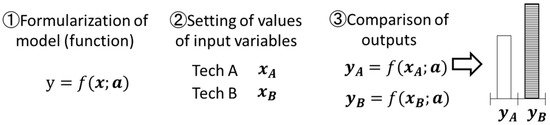
Figure 1. Conventional LCI procedure.

(1)

Formulate a model to evaluate specific indices (e.g., life cycle CO₂ emission, life cycle cost).

(2)

Set values for the input variables constituting the model.

(3)

Determine the corresponding output values of the model and interpret the results for evaluation.

The values of input variables can be obtained by either surveying the literature or performing measurements to then derive the results. As noted above, results are fully dependent on the inputs (assumptions). Hence, when high uncertainty is related to inputs, one can argue that input values may be selected to direct the model toward the desired results.

2.1.2. Concept Adopted in this Study

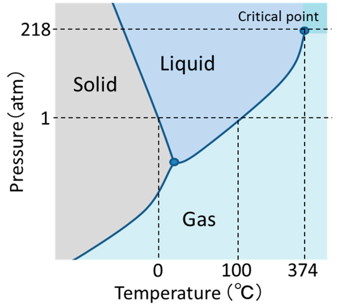
This study intended to provide a tool for the comprehensive visualization of relationships between inputs and outputs, specifically for evaluating HV and EV technologies. The basic concept is general and based on an approach similar to that used for constructing a water phase diagram (see Figure 2). This diagram shows the state of water (gas, liquid, or solid) according to two variables, namely, temperature and pressure, thus enabling the understanding of the state given any combination of the two variables. Similar diagrams would also contribute to understanding the LCI results. However, an LCI model consists of several variables, and visualization through multidimensional maps is thus required.

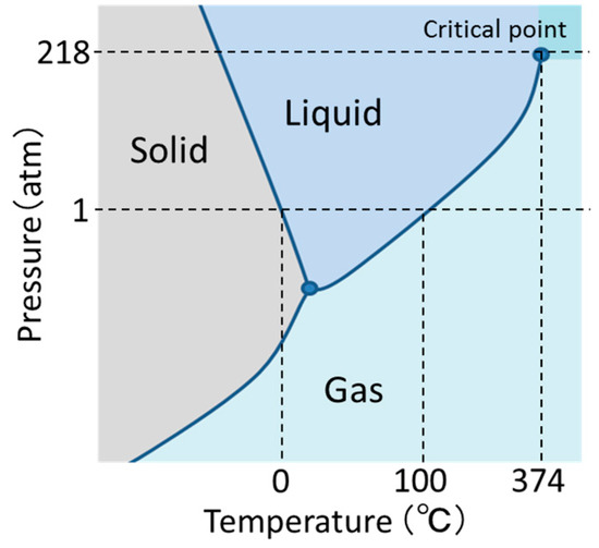
Figure 2. Phase diagram of water.

2.2. Problem Setting

In this paper, I compare LCC and LCCO₂ between HVs and EVs applying the developed visualization methodology.

2.2.1. Model

The LCC of HVs and EVs is given by

$$y_{HV}=C_{HV}+\frac{P_{gas}}{E_{HV}}L,$$

(1)

$$y_{EV}=C_{EV}+\frac{P_{elec}}{E_{EV}}L,$$

(2)

where

$y_i$ = LCC of vehicle type $i$ ($i=HV\mathrm{or}EV$),

$C_i$ = vehicle cost,

$E_i$ = energy efficiency,

$P_j$ = price of energy source $j$ ($j=gas\mathrm{or}elec$), and

$L$ = total mileage travelled.

Many other important factors can be analyzed regarding LCC of vehicles, e.g., maintenance cost and resale value. For simplicity, the proposed LCC model does not explicitly reflect these factors, but the vehicle cost can incorporate the resale value and maintenance cost provided that these factors are estimated beforehand.

Equations (1) and (2) are depicted in Figure 3, and their combination retrieves

$$\mathsf{\Delta }y=\mathsf{\Delta }C+\left(\frac{P_{elec}}{E_{EV}}-\frac{P_{gas}}{E_{HV}}\right)L,$$

(3)

where $\mathsf{\Delta }y=y_{HV}-y_{EV}\mathrm{and}\mathsf{\Delta }C=C_{HV}-C_{EV}$. Equation (3) describes seven variables, six inputs and one output, with variables not being distinguishable from parameters.

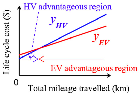
Figure 3. LCC comparison between HV and EV.

Similarly, the LCCO₂ for HVs and EVs is given by

$$z_{HV}=D_{HV}+\frac{Q_{gas}}{E_{HV}}L,$$

(4)

$$z_{EV}=D_{EV}+\frac{Q_{elec}}{E_{EV}}L,$$

(5)

where

$z_i$ = LCCO₂ of vehicle type $i$ ($i=HV\mathrm{or} EV$),

$D_i$ = vehicle CO₂ emission during production (derived from the processes of vehicle production including raw materials, manufacturing of parts, and assembly), and

$Q_j$ = CO₂ intensity of energy source $j$ ($j=\mathrm{gasoline}\mathrm{or}\mathrm{elec}tricity$). This variable includes CO₂ emissions from fuel production and transport and can be thus considered as the well-to-wheel CO₂ intensity.

Combining Equations (4) and (5) retrieves

$$\mathsf{\Delta }z=\mathsf{\Delta }D+(\frac{Q_{elec}}{E_{EV}}-\frac{Q_{gas}}{E_{HV}})L,$$

(6)

where $\mathsf{\Delta }z=z_{HV}-z_{EV}\mathrm{and}\mathsf{\Delta }D=D_{HV}-D_{EV}$. Equation (6) also describes seven variables (six inputs and one output, where variables are not distinguishable from parameters). The proposed model does not assume correlations among input variables, i.e., all variables can be treated as independent and are not affected by other factors.

2.2.2. Ranges of Variables

The ranges of the variables used in this study are listed in Table 1. These settings (including the units) can be changed depending on the purpose. The GREET model [11] was the reference to set the values of vehicle CO₂ emissions during production and CO₂ intensity of the energy source.

Table 1. Ranges of variables for LCC analysis.

Variable	Unit	Min.	Max.
Fuel efficiency of HV	km/L	20	40
Energy efficiency of EV	km/kWh	5	15
Total mileage travelled (lifetime)	km	30,000	100,000
Difference in vehicle price	$	1000	10,000
Gasoline price	$/L	0.5	2.0
Electricity price	$/kWh	0.1	0.25
Difference in vehicle CO2	kgCO2	500	4000
CO2 intensity of gasoline	kgCO2/L	2.5	3.2
CO2 intensity of electricity	kgCO2/kWh	0.2	0.8

3. Results

3.1. LCC

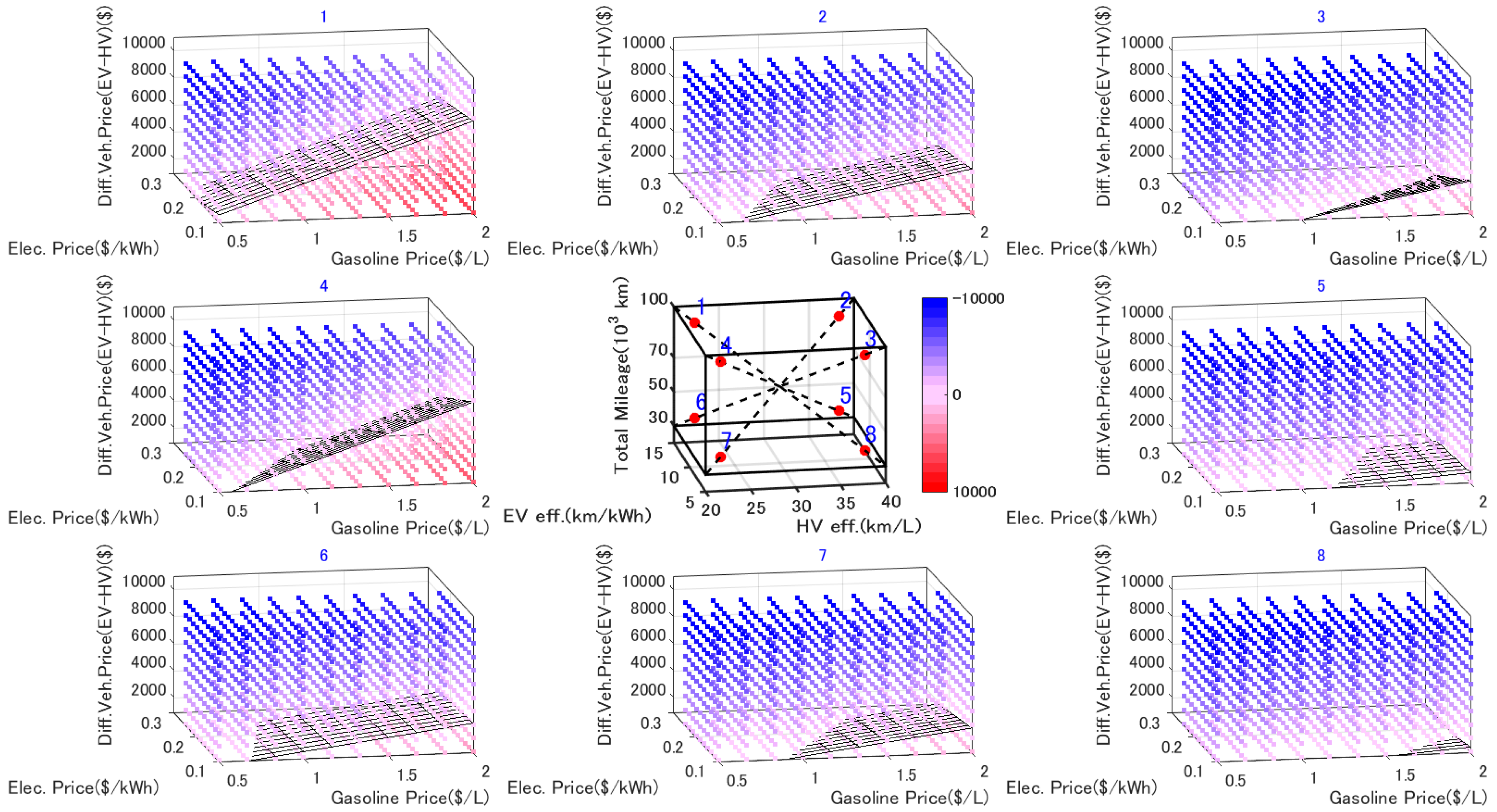
Figure 4 shows the result of the comprehensive comparison of LCC between HV and EV, or a visualization of Equation (3). Different combinations of values of the six input variables, i.e., HV fuel efficiency, EV energy efficiency, total mileage, gasoline price, electricity price, and difference in vehicle price, are considered. The settings of the first three variables are shown in the center as a cube with eight points within it. Each point corresponds to the settings of the three variables of each of eight 3D diagrams around the center.

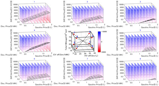
Figure 4. Six-dimensional diagram of comprehensive LCC comparison between HV and EV (regions colored in blue and red represent advantageous HV and EV, respectively).

These eight 3D diagrams around the center show the corresponding relationships between difference of LCC, $\mathsf{\Delta }y$, and the last three variables with fixed values of the first three variables. Different values of $\mathsf{\Delta }y$ are represented by different colors; a negative value, indicating that the LCC of HV is lower (i.e., HV is advantageous) is represented in blue, while a positive value, indicating that the LCC of EV is lower, is represented in red. Near zero values are shown in magenta. Black planes represent thresholds at which the LCC of HV and EV is equal.

It is apparent that the blue colored region is larger than the red one, indicating that the advantageous region of HV is larger than that of EV in terms of LCC. Based on a comparison of 3D diagrams nos. 1 and 4, the better the EV energy efficiency, the larger the advantageous EV region. Similarly, the worse the HV fuel efficiency or the longer the total mileage, the better the EV energy efficiency. However, even taking these conditions into account, HV is advantageous if EV price is $8000 or more than that of HV.

3.2. LCCO₂

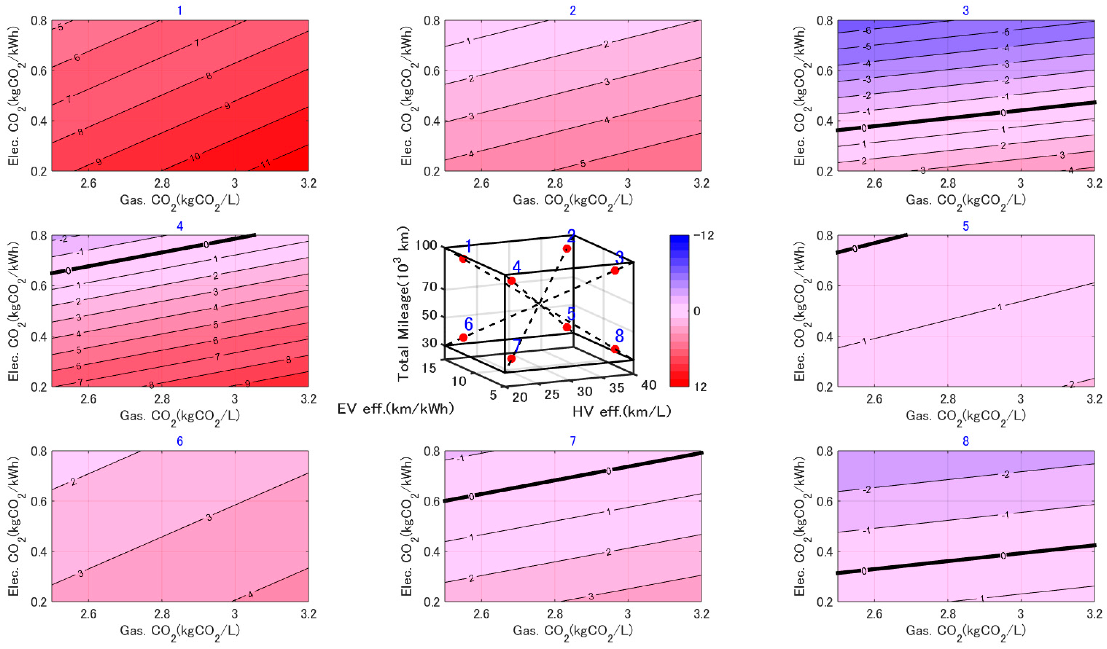
Figure 5 and Figure 6 show the result of the comprehensive comparison of LCCO₂ between HV and EV, or a visualization of Equation (5). Different from the case of Figure 4, the difference in vehicle CO₂, $\mathsf{\Delta }D$, is treated as constant, and two cases (lower and higher case) are shown in Figure 5 and Figure 6, respectively. The figure thus consists of a combination of a 3D diagram representing three common variables (HV fuel efficiency, EV energy efficiency, and total mileage) in the center, and 2D contour diagrams showing the relationships between difference in LCCO₂, $\mathsf{\Delta }z$, and the other two input variables (gasoline and electricity CO₂ intensity). For ease of understanding, the dimension of diagrams around the center is reduced to 2D by treating $\mathsf{\Delta }D$ as constant. The colors used to indicate the relative advantages of HV and EV are the same as in Figure 4; blue represents the HV advantageous region, while red indicates advantageous EV. The ranges of gasoline and electricity CO₂ intensities are the same in the eight 2D diagrams.

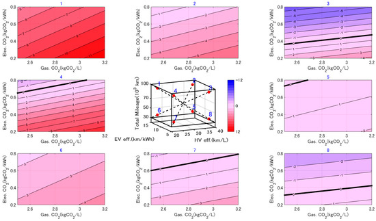
Figure 5. Five-dimensional diagram of comprehensive LCCO₂ comparison between HV and EV with difference of vehicle CO₂ emissions during production $\mathsf{\Delta }D$ set to 500 kg.

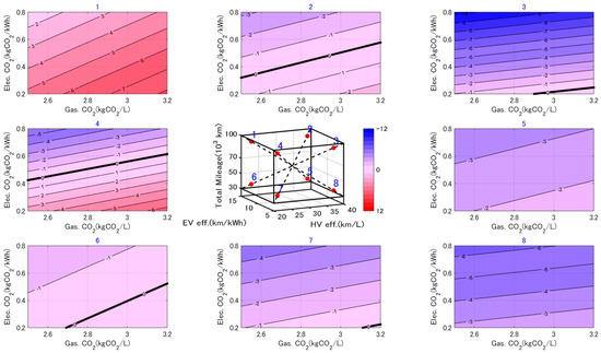
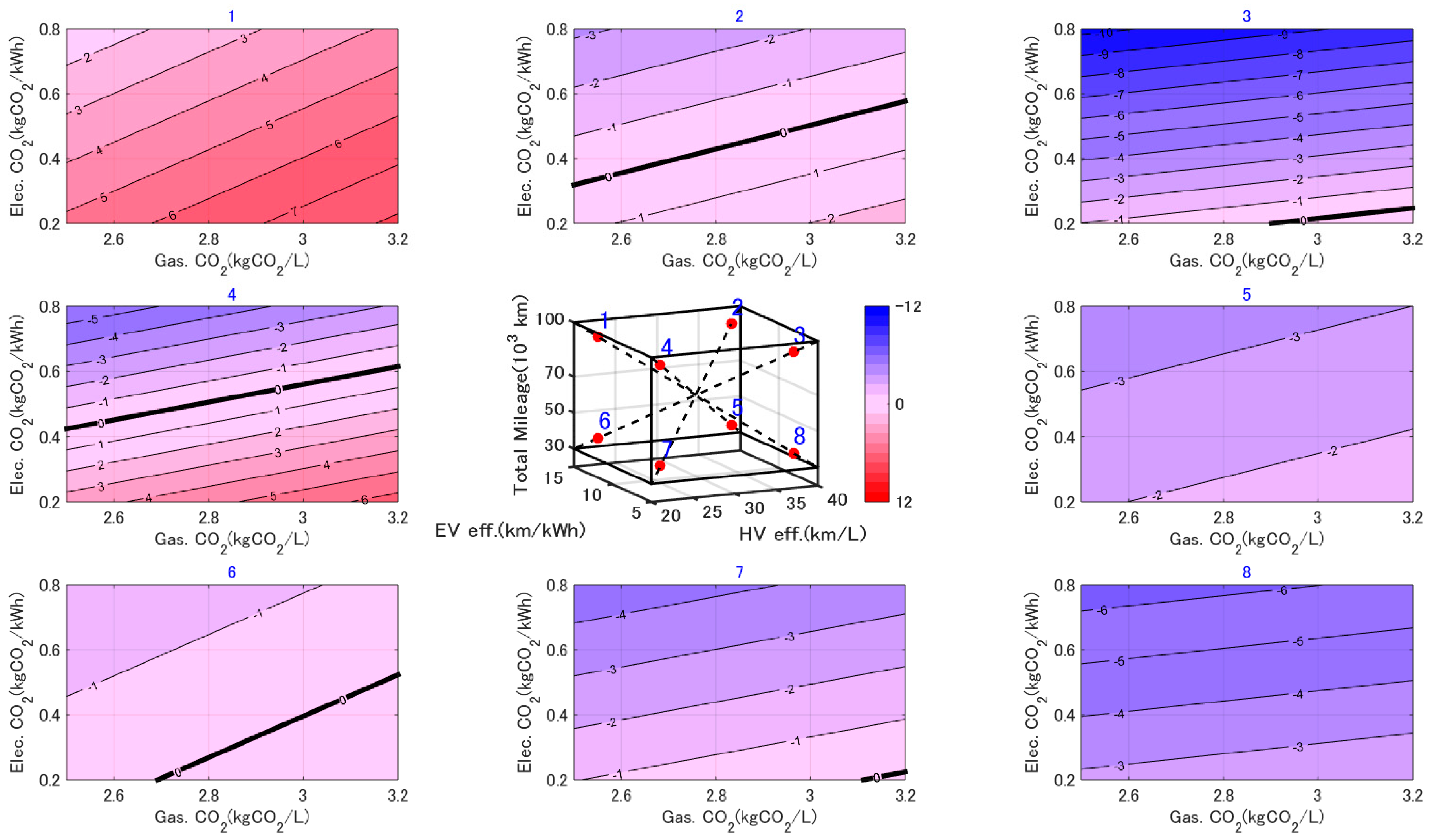
Figure 6. Five-dimensional diagram of comprehensive LCCO₂ comparison between HV and EV with difference of vehicle CO₂ emissions during production $\mathsf{\Delta }D$ set to 4000 kg.

The coloring of 2D diagrams evidently differs depending on the combination of values of three common variables and the difference in vehicle CO₂. The key conclusions that can be drawn from Figure 5 and Figure 6 are summarized as follows.

(1)

EV is advantageous in almost all areas (combinations of the ranges of gasoline and electricity CO₂ intensity) of 2D diagrams Nos. 1, 2, 5, and 6 in Figure 5, and No. 1 in Figure 6. That means:

(1)

when EV energy efficiency is better (about 15 km/kWh or more) and total mileage is adequate, EV is advantageous regardless of HV fuel efficiency, and

(2)

the extent of EV’s advantage is increased when gasoline CO₂ intensity is greater, or when electricity CO₂ intensity is lower.

(2)

Comparing Figure 5 and Figure 6, or the diagrams with different settings of $\mathsf{\Delta }D$, the coloring of each diagram differs but the width of contours remains the same. This is because the difference between the two figures is an intercept of the comparison of LCCO₂ of HV and EV.

(3)

When assuming HV and EV efficiency at current levels (No. 4 in Figure 3 and Figure 4), then HV is advantageous in the region of larger electricity CO₂ intensity (about 0.8 kgCO₂/kWh or more).

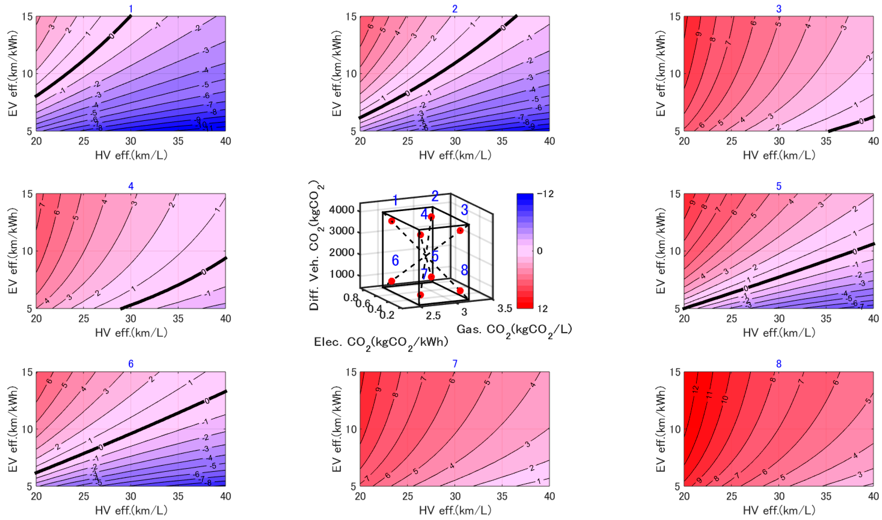
3.3. LCCO₂ Analysis on Different Axes

Figure 7 and Figure 8 show different variable combinations. The three variables in the central graph represent gasoline CO₂ intensity, electricity CO₂ intensity, and difference of vehicle CO₂ emissions during production, and the axes of the 2D contour diagrams show HV and EV efficiency. In the figures, the total mileage travelled is constant, respectively considering 30,000 and 100,000 km for Figure 7 and Figure 8.

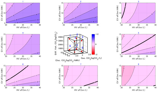
Figure 7. Five-dimensional diagram of LCCO₂ comparison emphasizing vehicle efficiency with difference of vehicle CO₂ emissions during production $\mathsf{\Delta }D$ set to 500 kg.

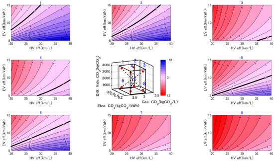
Figure 8. Five-dimensional diagram of LCCO₂ comparison emphasizing vehicle efficiency with difference of vehicle CO₂ emissions during production $\mathsf{\Delta }D$ set to 4000 kg.

Unlike Figure 5 and Figure 6, the contour curves do not exhibit a linear trend. In the region where electricity CO₂ intensity is higher, the coloring of diagrams varies, indicating that the relative advantage of the vehicles is highly dependent on both HV and EV efficiency.

3.4. Application to Regional Scenario Analyses

As gasoline and electricity prices and CO₂ intensities generally differ among regions, the comparisons would also differ among regions, even under the same technological assumptions. This methodology, which represents specific values of regions as points plotted on the diagrams, enables a comprehensive understanding of the extent to which a given vehicle is advantageous under any combination of assumptions.

Two regions in the United States with different properties, California and the Midwest, are considered as an example. Coal power is the main source of energy in the Midwest whereas renewables are extensively deployed in California. Table 2 shows the settings of energy prices and CO₂ intensities for the two regions.

Table 2. Values for some vehicle variables in the Midwest and California, US.

Variable	Midwest	California	Study
Gasoline Price ($/L)	0.581	0.740	[12]
Electricity Price ($/kWh)	0.126	0.177	[12]
Gasoline CO2 intensity (kgCO2/L)	3.05	3.05	[6]
Electricity CO2 intensity (kgCO2/L)	0.799	0.299	[13]

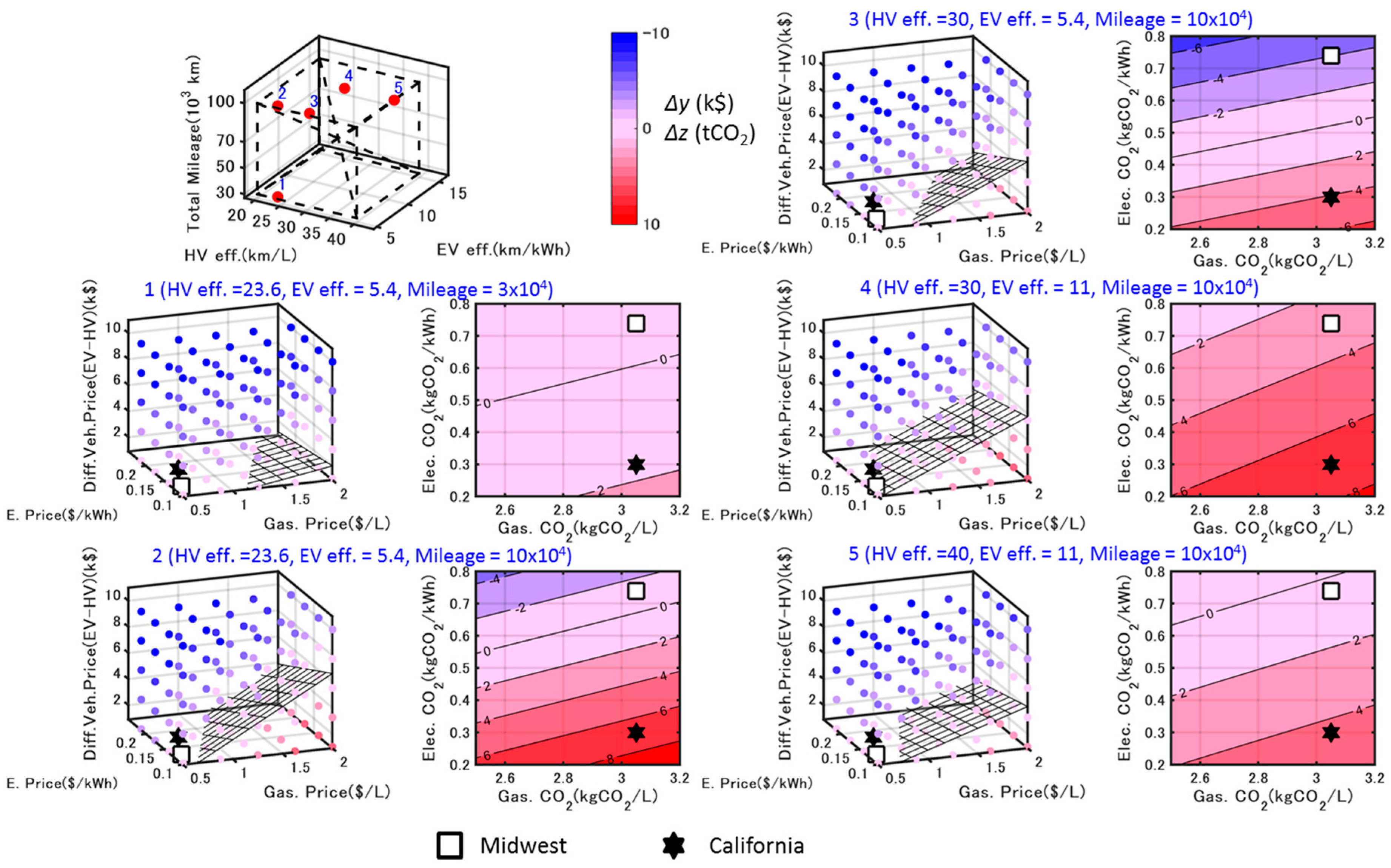
By combining the two diagrams for LCC and LCCO₂, I constructed an eight-dimensional diagram with three common variables, three price variables, and two CO₂ intensity variables. Plotting the points representing the two regions and considering different combinations of the common variables illustrate the variation of techno-economic outcomes among regions, as shown in Figure 9. For simplicity, the difference in vehicle price at these two regions was considered to be $1000 for LCC, and the difference in vehicle CO₂ emissions during production was considered low (500 kg) for LCCO₂.

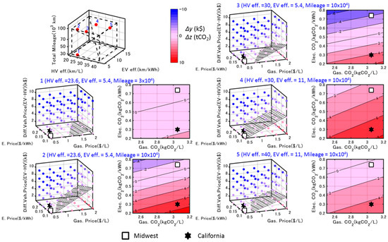
Figure 9. Eight-dimensional diagram representing specific regions showing the LCC and LCCO₂ comparisons between HV and EV under five different settings of fuel efficiency and total mileage travelled.

The top left graph in Figure 9 depicts HV fuel efficiency, EV energy efficiency, and total mileage travelled. Points 1 to 5 within the figure correspond to the settings of the variables of each pair of 3D and 2D diagrams for LCC and LCCO₂, respectively.

Point 1 (in the top left graph) shows the initial setting for HV fuel efficiency and EV energy efficiency for the corresponding diagrams. The mileage travelled was set to 30,000 km, assuming a total cost and CO₂ emissions over three years with annual mileage travelled of 10,000 km. The diagram at the left of the second row indicates that HVs are advantageous for both regions in terms of LCC, whereas the Midwest and California are the most advantageous for HVs and EVs, respectively, for LCCO₂.

Point 2 (in the top left graph) changes the total mileage travelled to 100,000 km. The corresponding diagram at the left of third row indicates that for the LCC, HVs are still advantageous for both regions, although the distance to the threshold plane is closer than that at point 1. In addition, the width of contour in the LCCO₂ diagram is narrower than that at point 1, suggesting that the difference in LCCO₂ increases for HVs and EVs at the same setting.

The HV fuel efficiency improves from diagram 2 to 3, whereas the EV energy efficiency improves from diagram 3 to 4. Diagram 4 shows that the two regions are almost on the threshold for LCC (i.e., EVs become cost competitive with HVs), whereas for LCCO₂, the Midwest also becomes advantageous for EVs. HV fuel efficiency further improves from diagram 4 to 5. For LCC, both regions are again advantageous for HVs, but both regions are advantageous for EVs regarding LCCO₂.

Overall, HVs exhibit advantage in terms of LCC (see Figure 10, which summarizes the LCC results shown in Figure 9). For LCCO₂, the advantage of either type of vehicle depends on the combination of the settings, but EVs are advantageous if their energy efficiency is high, even in a region with CO₂ intensive electricity like the Midwest.

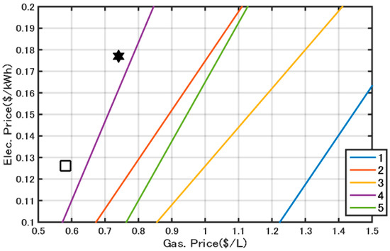
Figure 10. Two-dimensional diagram summarizing the LCC comparison shown in Figure 9. The relationships between points representing specific regions and threshold lines for each setting in Figure 9 are depicted for a difference in the vehicle price of $1000, that is, the diagram corresponds to the base of the cubes for the LCC space in Figure 9.

Figure 4, Figure 5, Figure 6, Figure 7, Figure 8, Figure 9 and Figure 10 were generated using a graphical user interface implemented on MATLAB to enable the interactive visualization of the analysis presented in this study. A supplementary movie supports the results shown in Figure 9.

4. Discussion

In this paper, I proposed a multi-dimensional techno-economic assessment diagram to comprehensively visualize the relationships between assumptions and results. I then demonstrated the application of the methodology to compare the LCC and LCCO₂ between HVs and EVs.

The results exhibit complicated relationships between assumptions and results even for simple functions, making it difficult to completely understand these relationships intuitively. Therefore, this methodology applied to relatively simple problems may facilitate the comprehensive understanding of relationships among variables.

Several studies compare conventional and alternative energy vehicles from economic and environmental viewpoints, such as life cycle assessment, techno-economic analysis, well to wheel analysis, and total cost of ownership (e.g., [2,3,4,5,13]). However, understanding the relationships between inputs and outputs is usually more important than focusing on the results of such evaluations, because the relationships depend on inputs (assumptions). In this context, the methodology presented here can contribute to comparing studies by summarizing meta-analyses of LCA studies and suggesting a procedure to create diagrams with points representing the results of different studies.

Furthermore, the presented methodology can be beneficial to finding critical factors or variables in such assessments. In the application example detailed in Section 3.4, EV energy efficiency was found to be key to LCCO₂. By visualizing specific settings as plots and dividing advantageous regions for HVs and EVs into threshold lines or planes, results under different conditions vary (e.g., the extent to which energy prices or CO₂ intensities change the advantageous type of vehicle). The distance between a point on the diagrams and the threshold might point toward targets for technology research and development or policy design that would render a specific technology advantageous.

The presented diagram can be extended to include other vehicle types (e.g., plug-in hybrid and fuel cell vehicles) and performance variables by including additional information, such as that considered by Hara et al. [14], who conducted a techno-economic analysis of alternative energy vehicles including solar hybrid vehicles.

References

- International Energy Agency. CO2 Emissions from Fuel Combustion Highlights 2014 Edition. Available online: https://www.iea.org/publications/freepublications/publication/CO2EmissionsFromFuelCombustionHighlights2014.pdf (accessed on 7 January 2017).
- Hawkins, T.R.; Gausen, O.M.; Strømman, A.H. Environmental impacts of hybrid and electric vehicles-a review. Int. J. Life Cycle Assess. 2012, 17, 997–1014. [Google Scholar] [CrossRef]
- Nordelöf, A.; Messagie, M.; Tillman, A.M.; Söderman, M.L.; Van Mierlo, J. Environmental impacts of hybrid, plug-in hybrid, and battery electric vehicles—What can we learn from life cycle assessment? Int. J. Life Cycle Assess. 2014, 19, 1866–1890. [Google Scholar] [CrossRef]
- Kamguia Simeu, S.; Brokate, J.; Stephens, T.; Rousseau, A. Factors Influencing Energy Consumption and Cost-Competiveness of Plug-in Electric Vehicles. World Electr. Veh. J. 2018, 9, 23. [Google Scholar] [CrossRef]
- Rupp, M.; Schulze, S.; Kuperjans, I. Comparative Life Cycle Analysis of Conventional and Hybrid Heavy-Duty Trucks. World Electr. Veh. J. 2018, 9, 33. [Google Scholar] [CrossRef]
- Hara, T.; Shiga, T.; Kimura, K.; Sato, A. Techno-Economic Analysis of Solar Hybrid Vehicles Part 2: Comparative Analysis of Economic, Environmental, and Usability Benefits. SAE Tech. Pap. 2016. [Google Scholar] [CrossRef]
- Fukushima, Y.; Hirao, M. LCA Methodology A structured framework and language for scenario-based life cycle assessment. Int. J. Life Cycle Assess. 2002, 7, 317–329. [Google Scholar]
- Barter, G.E.; Reichmuth, D.; Westbrook, J.; Malczynski, L.A.; West, T.H.; Manley, D.K.; Guzman, K.D.; Edwards, D.M. Parametric analysis of technology and policy tradeoffs for conventional and electric light-duty vehicles. Energy Policy 2012, 46, 473–488. [Google Scholar] [CrossRef]
- Chen, I.C.; Fukushima, Y.; Kikuchi, Y.; Hirao, M. A graphical representation for consequential life cycle assessment of future technologies-Part 2: Two case studies on choice of technologies and evaluation of technology improvements. Int. J. Life Cycle Assess. 2012, 17, 270–276. [Google Scholar] [CrossRef]
- Braff, W.A.; Mueller, J.M.; Trancik, J.E. Value of storage technologies for wind and solar energy. Nat. Clim. Chang. 2016, 6, 964–969. [Google Scholar] [CrossRef]
- Argonne National Laboratory. GREET 1 and GREET 2 2014. Available online: https://greet.es.anl.gov/ (accessed on 1 October 2015).
- U.S. Energy Information Administration. Available online: https://www.eia.gov/state/ (accessed on 1 June 2016).
- Tamayao, M.A.; Michalek, J.J.; Hendrickson, C.; Azevedo, I.M. Regional variability and uncertainty of electric vehicle life cycle CO2 emissions across the United States. Environ. Sci. Technol. 2015, 49, 8844–8855. [Google Scholar] [CrossRef] [PubMed]
- Hara, T.; Kimura, K.; Kudoh, Y.; Sato, A. Techno-Economic analysis of solar hybrid vehicles. In Proceedings of the 33rd Conference on Energy, Economy, and Environment, Tokyo, Japan, 3 February 2017; pp. 433–438. (In Japanese). [Google Scholar]
© 2018 by the author. Licensee MDPI, Basel, Switzerland. This article is an open access article distributed under the terms and conditions of the Creative Commons Attribution (CC BY) license (http://creativecommons.org/licenses/by/4.0/).