Collaborative Optimization Method of Structural Lightweight Design Integrating RSM-GA for an Electric Vehicle BIW

Abstract

The body-in-white (BIW) is an important part of the electric vehicle body, its mass accounts for about 30% of the vehicle mass, and reducing its mass can significantly contribute to energy savings and emission reduction. In this paper, a collaborative optimization method combining the response surface method and genetic algorithm (RSM-GA) is developed to perform the lightweight optimization of the body-in-white of an electric vehicle. Seventeen design variables were screened by relative sensitivity calculations based on modal and stiffness sensitivity analysis, and the data samples were collected using the Taguchi experiment and Hammersley experiment during the designing of the experiment methods. To further maintain the accuracy rate, the least squares regression, moving least squares method, and radial basis function are applied to fitting data to obtain the response surface, and the error analysis of the fitting results is carried out to correct the response surface. Finally, the genetic algorithm based on the response surface is employed to optimize the structure of the body-in-white, and the results are compared with those of the adaptive response surface method and sequential quadratic programming method. Through comparison, the paper found that the optimization effect obtained by the proposed method has a relatively high accuracy rate.

1. Introduction

With the rapid development of global science and technology, electric vehicles have become an important means of transportation for people’s daily travel. However, with the production and manufacturing of the machinery industry, we are also facing the energy crisis and ecological environmental pollution; energy savings and emission reduction in automobiles is an important issue facing society [1,2,3]. A large number of automobile manufacturing industries have taken the lightweight design of the body-in-white as a key research direction, and the lightweight design of the vehicle body helps to enhance the fuel efficiency, power performance, braking performance, and road durability of the car. It is of great significance for both traditional-fuel vehicles and new-energy vehicles, and is a key focus of the current automotive industry competition. The lightweight optimization design of the electric vehicle BIW covers a variety of disciplines, not only to reduce weight but also to ensure that the overall performance quality meets the design standards [4,5,6,7].

Structural optimization is an important method to obtain light weight that involves multiple levels of improvement. In the preliminary design stage, the finite element analysis (FEA) method is used to model and analyze the vehicle body structure, and the nodes and sections are optimized based on the stress distribution of the structure. By using topology optimization technology, a reasonable layout of materials in the structure can be achieved, thereby reducing the weight of the structure while meeting the design requirements. For example, Park et al. [8] conducted lightweight optimization design for the track rods of the rear chassis module of an automobile. Firstly, through analysis, they decided to replace the steel track rods with aluminum ones. Then, they used finite element analysis and optimization to determine the height and thickness of the ribs. Bastien et al. [9] took mass minimization as the design goal to carry out a lightweight design of the BIW. Through the experiment, they found that using the moving least square approximation model is better. In the detailed design stage, shape optimization and size optimization methods are used to optimize the specific vehicle body structure in detail. The combined application of these optimization methods helps to ensure the satisfaction of safety, performance, and other requirements, and to achieve a structural lightweight design of the BIW.

Due to the numerous variables and complex constraints of the multi-disciplinary optimization of the vehicle body, along with its strong nonlinearity, it is usually necessary to employ global optimal solution search algorithms for a solution. These algorithms involve thousands of iterations during the optimization process. If direct simulation is called upon, it will consume an enormous amount of computing resources and time. The surrogate model method is one of the effective approaches to solving these problems. The surrogate model method refers to a mathematical modeling approach that uses an approximate method to fit discrete data to establish a continuous functional relationship between input and output [10,11,12]. Under the premise of meeting the accuracy requirements, using the surrogate model to replace the costly simulation for optimization can significantly reduce the computing cost and improve the optimization efficiency; meanwhile, common surrogate models include response surface models, particle swarm optimization (PSO), back-propagation neural networks (BPNNs), etc. Many scholars have begun to utilize proxy models to establish optimization algorithms for the lightweight design of structures. Kiani et al. [10] took the BIW as their research object and used a Latin hypercube to collect experimental data and build a surrogate model. Under the condition of meeting the requirements of vibration and stiffness, the noise vibration and harshness (NVH) performance of the optimized vehicle was improved. Duan et al. [11] proposed a thick-based subdomain hybrid cellular automata (T-SHCA) algorithm to carry out lightweight optimization of the BIW under side impact conditions. Experimental results showed that the T-SHCA algorithm can effectively solve the nonlinear dynamic response optimization problem. Topa M et al. [12] carried out a lightweight design of the connecting bracket of the chassis and rear axle, reducing the stress value of the connecting bracket and reducing its mass by 63% through the response surface method and topology optimization. Hong et al. [13] proposed a stress-based structural optimization method, using AlSi10Mg alloy materials and selective laser melting to manufacture lightweight parts. The experimental results showed that the upper limit of load of the designed structure is increased by 15.25%. Xiong et al. [14] carried out a multi-objective lightweight design of the front-end structure and material of the automobile body and used the hybrid method of the multi-objective particle swarm optimization algorithm and TOPSIS algorithm to optimize the model, and the final structure mass was reduced by 4.12 kg than before. Guler et al. [15] developed an automobile hinge component using a glass fiber composite material instead of traditional steel. The topological optimization under a specific load is carried out by the finite element method, and the weight of the component is reduced under the conditions of displacement and stress. Lu et al. [16] carried out a lightweight design of the bus frame, taking material and size as variables, and stiffness and frequency as constraints. The sequential linear programming method was used for optimization and validated by engineering experiments. Zhou et al. [17] researched laser spiral welding, taking welding parameters as design variables, and by using the genetic algorithm for optimization, the tensile strength of the weld joint increased by 8% and the plasticity increased by 25%.

Among the optimization algorithms, the GA, PSO, and BPNN methods have a better optimization effect. Researchers have used these optimization algorithms and their combined methods (such as RSM-GA, GA-BP, etc.) to solve engineering problems in a variety of fields, such as software safety, optimization design, and object detection [18,19,20,21,22]. PSO relies on the sharing of information among particles. Although it can converge quickly, it is prone to becoming stuck in local optima in complex multi-modal problems [18]. The BPNN requires a large amount of data for training, and the randomness of the initial weights makes parameter optimization difficult [19]. RSM-GA combines the efficient modeling capability of RSM with the global search feature of GA, and is suitable for handling complex nonlinear and multi-modal optimization problems. It performs particularly well in engineering scenarios where data is scarce or rapid convergence is required [20,21]. Compared with a single RSM or GA, RSM-GA enhances the optimization accuracy and efficiency through a complementary mechanism; compared with methods such as PSO and neural networks, RSM-GA has significant advantages in model interpretability, data requirements, nonlinear processing capabilities, and engineering verification reliability. Therefore, this paper will use the RSM-GA as the optimization algorithm.

In this paper, the genetic algorithm based on the response surface is used to optimize the lightweight design of the passenger car BIW. Firstly, the modal, stiffness, and strength of the BIW are analyzed by the finite element method to determine its characteristics. Secondly, the design variables are screened based on the relative sensitivity calculation of sensitivity analysis. Then, the Taguchi experiment and Hamersley experiment in the design of experiment (DOE) methods were used to provide the data for creating the response surface, and the least squares regression (LSR), moving least squares (MLS), and radial basis function (RBF) were used to fit the response surface, and the accuracy of the response surface was verified by error analysis. Finally, the lightweight optimization design of BIW is carried out based on the genetic algorithm of the response surface, and the optimization results are compared with the adaptive corresponding surface method and the sequential quadratic programming method to verify the superiority of the proposed scheme.

The outline is as follows: The second part introduces the genetic algorithm and the genetic algorithm based on the response surface. The third part describes the establishment of the finite element model of BIW and the process and results of modal analysis, stiffness analysis, and strength analysis. The fourth part describes the sensitivity analysis and relative sensitivity calculation process, according to which the design variables are screened. The fifth part provides experimental data by using the Taguchi experiment and Hamersley experiment, and uses experimental data to fit the response surface model, and carries out error analysis to verify the accuracy of the response surface model. The sixth part optimizes the BIW model based on the response surface of the genetic algorithm, and the superiority of this method is verified by comparing the optimization results with the adaptive response surface method and the sequential quadratic programming method. Finally, the conclusions and prospects of this article are presented.

2. Methodology

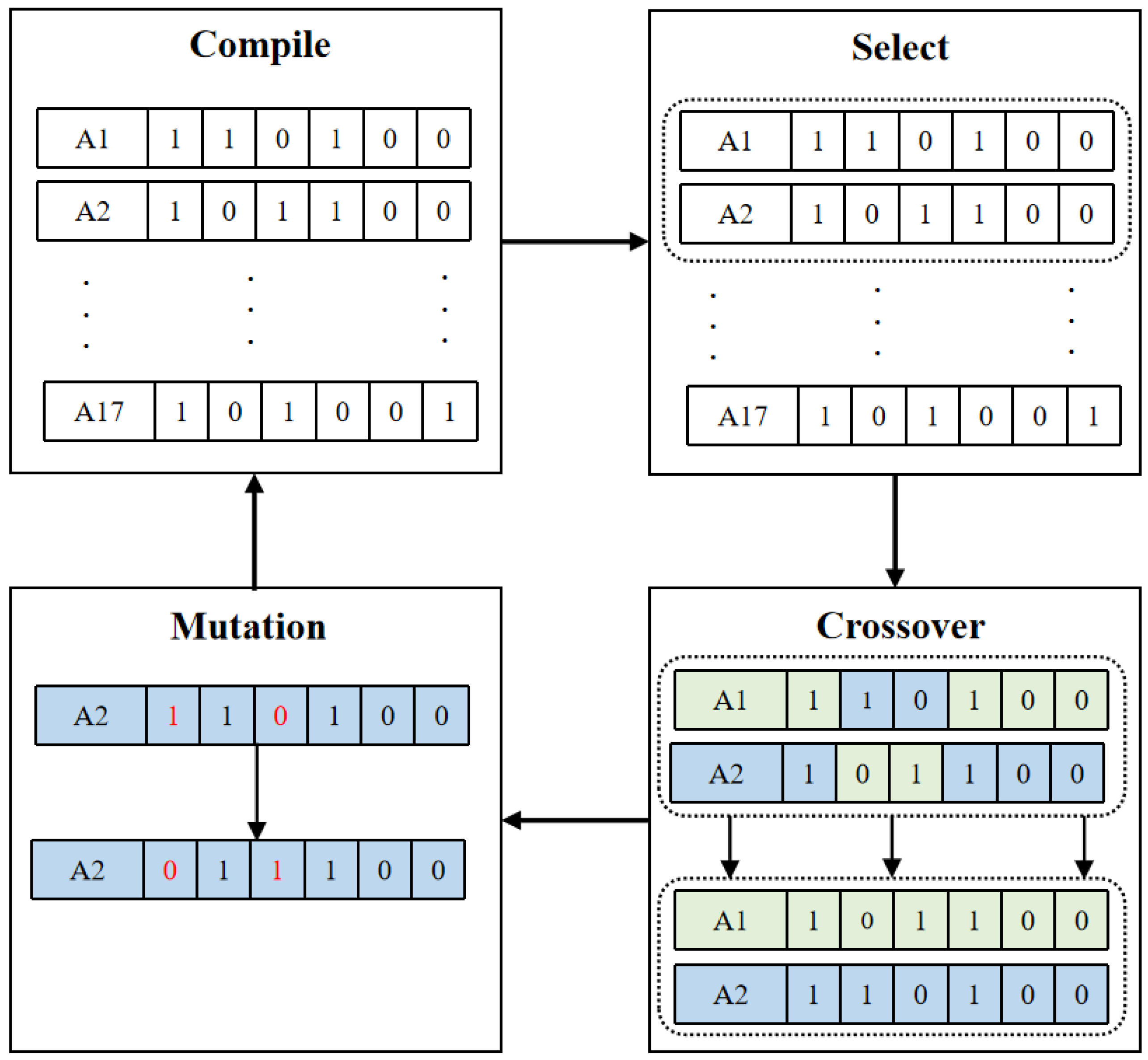
2.1. Genetic Algorithm

The genetic algorithm is an adaptive global optimization algorithm formed by observing the heredity and evolution of organisms [23]. Based on the crossover and mutation of chromosomes during the biological evolution process, and by using genetic operations to manipulate the population, selection operations, crossover operations, and mutation operations are carried out to obtain a new generation of the population (as shown in Figure 1).

Genetic operators in genetic algorithms include selection operators, crossover operators, and mutation operators, which continuously evolve by using genetic operators to generate new populations (as shown in Figure 2).

(1) 

Selection operator: The selection operator is based on the fitness evaluation method. By inheriting the individuals with high fitness in the population, the selection operator can avoid gene loss and improve global convergence and computing efficiency. Commonly used methods include fitness proportional selection or Monte Carlo selection (shown in Formula (1)), best individual preservation, and the expected value method.

$$P_i={\displaystyle \frac{F_i}{{\displaystyle \sum _{i=1}^n{F}_i}}}\hspace{0.17em}\hspace{0.17em}\hspace{0.17em}\hspace{0.17em}\hspace{0.17em}\hspace{0.17em}\hspace{0.17em}\hspace{0.17em}\hspace{0.17em}(i=1,2,3,\cdots ,n)$$

(1)

In Formula (1): P_i—the probability of individual i being selected; F_i—fitness of individual i.

(2) 

Crossover operator: The crossover operator is used in the genetic algorithm to generate new individuals, and two new chromosomes are generated through the exchange of several gene values on two chromosomes. The last three gene values of the two chromosomes are exchanged to produce two new chromosomes.

(3) 

Mutation operator: Mutation operation simulates the mutation of natural genes, and the mutation in binary coding is to reverse the gene on some loci, replacing 0 with 1 or replacing 1 with 0.

$$x_i^{\ast }=x_{i\min }+r\cdot (x_{i\min }+x_{i\max })$$

(2)

where $x_i^{\ast }$ represents the mutated gene value. $x_{i\min }$ is the lower limit value for the point of variation. $x_{i\max }$ denotes the upper limit value for the point of variation. r is a random number within the range of [0, 1] that conforms to a uniform probability distribution.

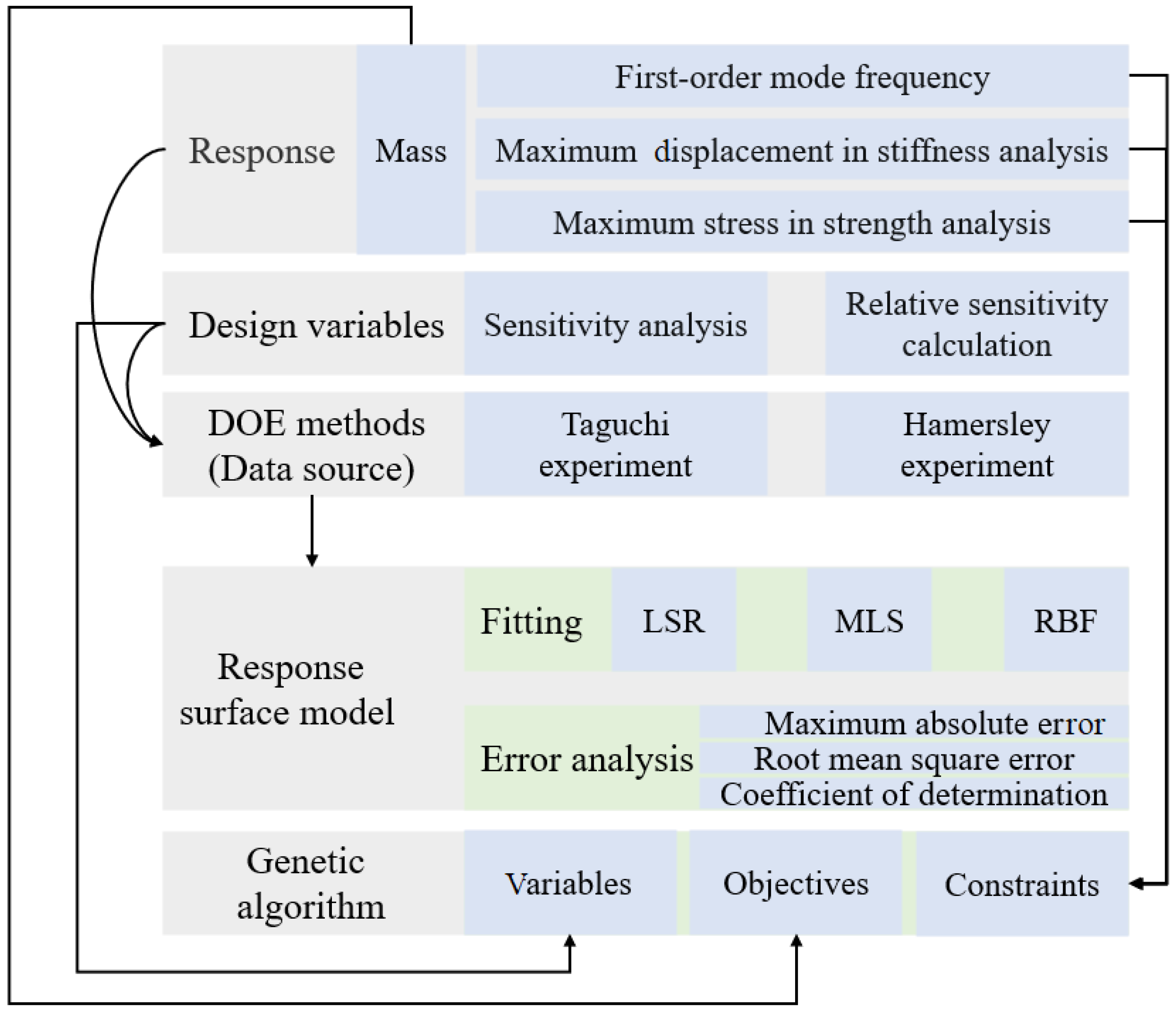
2.2. Genetic Algorithm Based on the Response Surface

The lightweight design of the BIW is based on the genetic algorithm of the response surface (as shown in Figure 3). Before this, variables and responses need to be set. The mass and first-order mode frequency, the maximum displacement in the stiffness analysis, and the maximum stress in the strength analysis are taken as responses in the finite element analysis. The design variables are screened by sensitivity analysis and relative sensitivity calculations. To construct the response surface model, we used the Taguchi experiment and Hammersley experiment in the DOE methods to collect data samples and fit the data through LSR, MLS, and RBF to construct the response surface model. At this time, we used the maximum absolute error, root mean square error, and coefficient of determination to conduct an error analysis of the response surface model to verify its accuracy. We can replace the finite element model with the response surface model, take the minimum mass as the goal, and other responses as constraints, and use the genetic algorithm to optimize the solution based on the response surface model to obtain a set of optimal solutions. Then this group of optimal solutions is used for finite element analysis, on the one hand, to see the error between the optimization results of the genetic algorithm based on response surface, and the finite element simulation results, on the other hand, to compare before and after optimization.

3. Model Building and Analysis

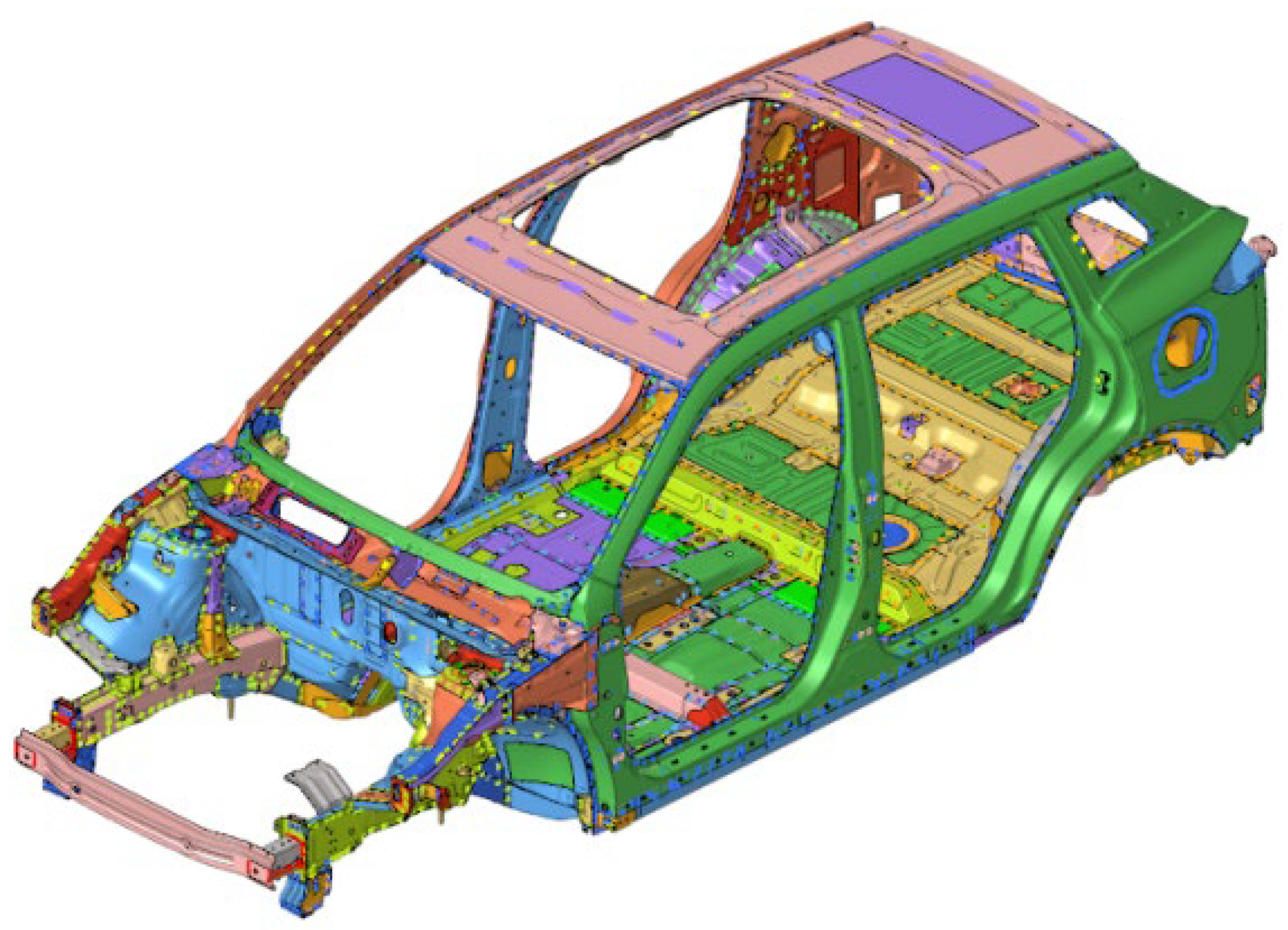
3.1. Model Building

Firstly, it is necessary to mesh the 3D model of the BIW, connect the parts, and set the material properties. The sheet metal parts of the BIW mainly include five materials (as shown in

Table 1. Material properties of the BIW components.

Material Type	Application Unit	Elastic Modulus (MPa)	Poisson Ratio	Density (t/mm3)	Yield Strength (MPa)
B280VK steel	Supporting part	207,000	0.3	7.83 × 10−9	280~420
B340DP steel	Pillar A, pillar B and pillar C	210,000	0.3	7.8 × 10−9	340~500
DC01 steel	Flooring	210,000	0.3	7.83 × 10−9	≥280
DCO4 steel	Car cowl panel	210,000	0.3	7.82 × 10−9	≥250
B240ZK steel	Other sheet metal parts	207,000	0.3	7.8 × 10−9	240~380

). By setting the material properties, the mechanical characteristics of each body component can be analyzed using the finite element method [24] to verify whether they meet the design requirements. Then, generate the finite element model of BIW (as shown in Figure 4), which is convenient for subsequent modal analysis, stiffness analysis, and strength analysis. During the process of establishing the finite element model, the first step is to preprocess the three-dimensional model of the vehicle body. Some minor features that do not affect the finite element analysis are ignored, and the sheet metal components are processed by extracting the meshing surface. Then, the finite element analysis model is established, and the quality of the divided finite element mesh is checked (

Table 2. Checklist for mesh quality.

Check Type	Display	Standard
Mesh edge length	Length	7.5–20 mm
Jacobi	Jcaobin	>0.7
Quadrilateral internal angle	Interior Angle Quad	40°~135°
Triangular internal angle	Interior Angle Tria	20°~120°
Skewness	Skewness	<60°
Aspect ratio	aspect ratio	3

). For those that do not meet the mesh quality requirements, modifications should be made.

3.2. Modal Analysis

Through modal analysis, the natural frequency and vibration type of the BIW can be determined. For the modal analysis of the BIW, no constraint conditions need to be set; it is conducted under free conditions. During the analysis process, low-frequency vibrations have a greater impact on the BIW, and the results of the first six orders are mainly analyzed and studied (as shown in Figure 5).

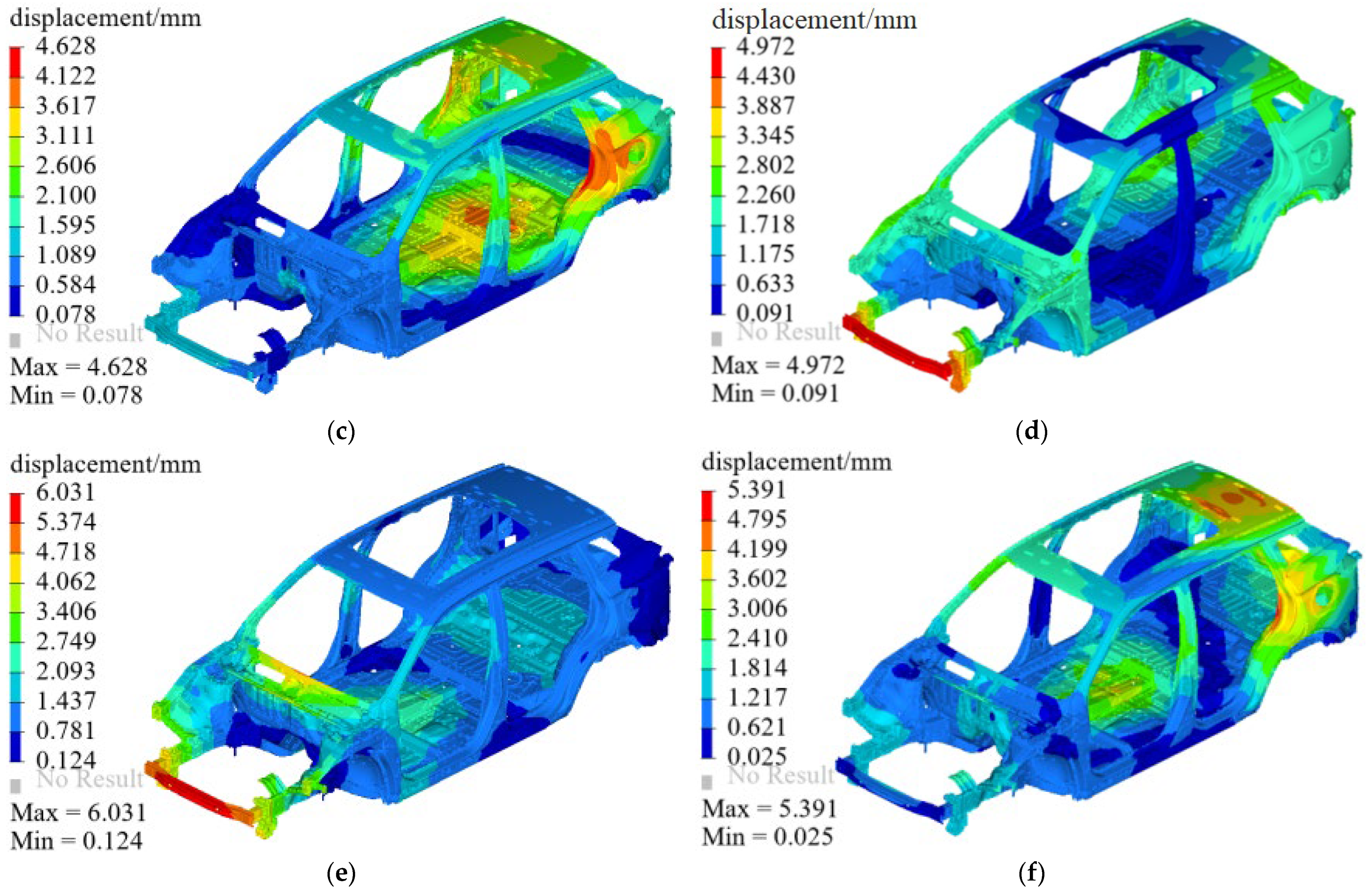
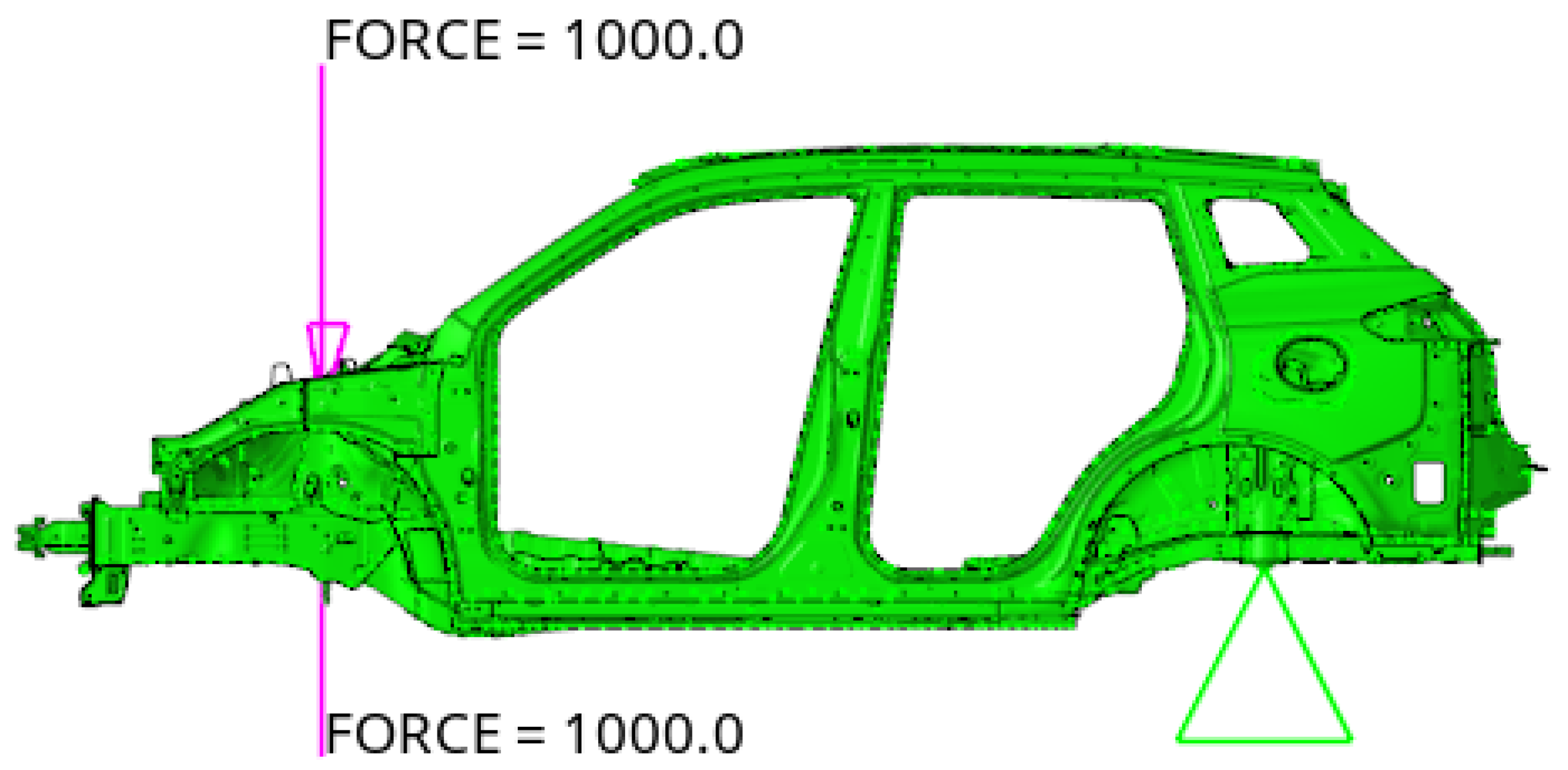
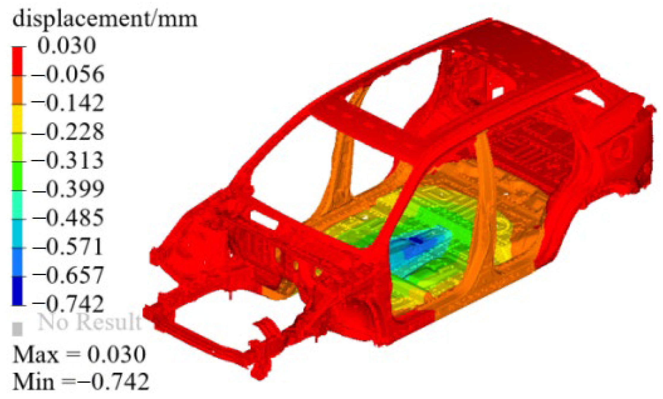
3.3. Stiffness Analysis

The BIW is a load-bearing body structure, which mainly bears a variety of loads from the road and passengers. Stiffness analysis studies the ability of the structure to resist deformation [10]. In the stiffness analysis, the bending stiffness and torsional stiffness are mainly analyzed. To facilitate the calculation of the stiffness value of the displacement deformation caused by the load of the BIW, 13 observation points are selected before and after the threshold beams on both sides, and a total of 26 observation points are selected, the stiffness value is calculated by measuring the displacement of the observation points (as shown in Figure 6, and the red dots represent the observation points).

The loads and constraints for the stiffness analysis are shown in Figure 7 and Figure 8, and the Z-axis cloud diagram in bending stiffness (Figure 9) and torsional stiffness (Figure 10) are obtained after calculation.

After collecting the displacement of 26 observation points, the bending stiffness of BIW is about 25,014.07 N/mm and the torsion stiffness is 22,410.39 N·m/°. The bending stiffness of the general SUV-type BIW is above 12,000 N/mm, and the torsional stiffness is above 15,000 N·m/°, so it meets the design requirements.

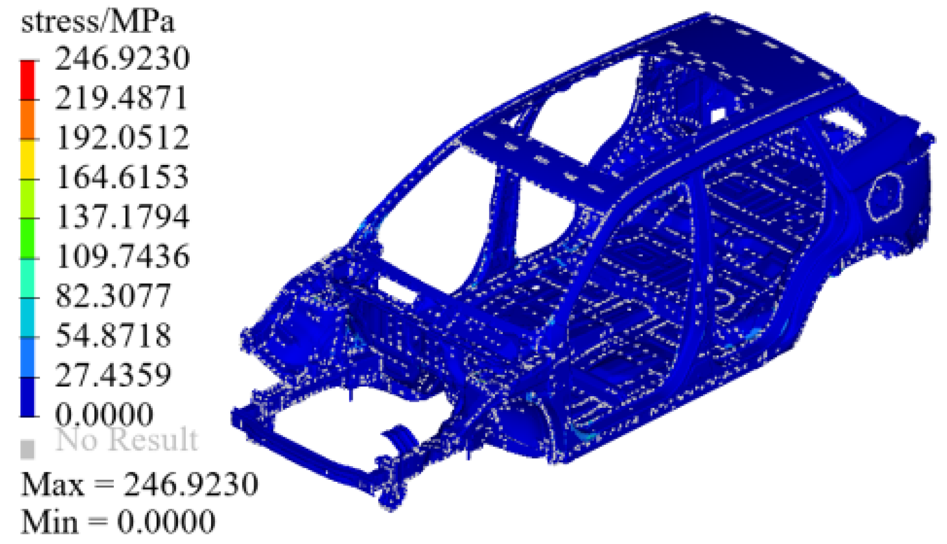
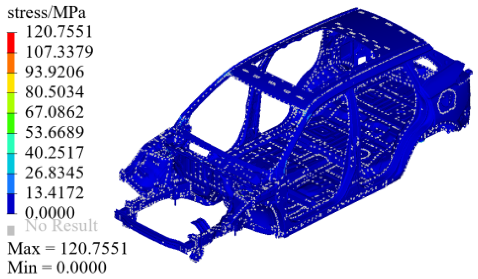
3.4. Analysis of Strength

Strength analysis studies the ability of the object structure to bear loads and the condition of local cracking or fracture of the object structure under the influence of various loads [25]. The strength analysis of the BIW can be used to check whether the bearing capacity of the BIW meets the strength design requirements. The strength analysis of the BIW in this paper mainly includes three working conditions of vertical impact, braking and steering, and the loads and constraints set (as shown in

Table 3. Load and constraint settings in the strength analysis.

Working Condition	Constrain				Load
	Constraint Position	X	Y	Z	X	Y	Z	g
Vertical impact	Left front suspension	✓	✓	✓	0	0	−3g	9800
	Right front suspension	✓		✓
	Left rear suspension		✓	✓
	Right rear suspension			✓
Braking	Left front suspension	✓	✓	✓	−1g		−1g	9800
	Right front suspension	✓	✓	✓
	Left rear suspension	✓	✓
	Right rear suspension	✓	✓
Steering direction	Left front suspension	✓	✓	✓		1g	−1g	9800
	Right front suspension	✓	✓	✓
	Left rear suspension	✓	✓	✓
	Right rear suspension	✓	✓	✓

). In the constraint process, X, Y, and Z represent translational degrees of freedom. In the load, X, Y, and Z represent the applied accelerations, and g represents the gravitational acceleration (9800 mm/s²). In Table 3, the ✓ indicates the imposition of constraints in that direction.

The stress cloud diagram of the vertical impact condition (shown in Figure 11), the brake condition (shown in Figure 12), and the steering condition (shown in Figure 13) were obtained by calculating the strength analysis.

After checking the analysis results, the maximum stress in the vertical impact condition is 221.2 MPa. The maximum stress under braking conditions was 246.92 MPa. The maximum stress in the turning condition was 120.75 MPa. Their maximum stress is less than the yield limit of the material, so it meets the design requirements.

4. Sensitivity Analysis and Relative Sensitivity Calculation

4.1. Sensitivity Analysis

Sensitivity analysis studies the sensitivity of an object or structure’s performance to design parameters [26,27], including global sensitivity analysis and local sensitivity analysis. Global sensitivity analysis is a method for evaluating the influence of model input parameters on model output. It not only considers the individual impact of a parameter at a specific point, but also takes into account the combined effect of all parameters and the changes throughout the parameter space. This analytical approach is of great significance for understanding the behavior of complex systems, optimizing model design, and conducting uncertainty quantification. It has been successfully applied in various fields, such as studying the dynamic modulus parameters of hot-mix asphalt mixtures and the seismic performance of shear walls [28,29]. The advantage of local sensitivity analysis is its simplicity in calculation and ease of understanding, which can help researchers understand the degree of influence of each parameter in the model on the results and optimize and adjust the parameters.

Design variables need to be selected before the optimization of the BIW, and reasonable panels should be selected for optimization through sensitivity analysis. The positive and negative value of sensitivity indicates the positive and negative correlation between the design variable and the response, and the absolute value of sensitivity indicates the severity of the influence of plate thickness on each working condition. In order to facilitate the intuitive observation of these parameters, the results of the nine sensitivity analysis scenarios are presented in a bar chart form (as shown in Figure 14). Here, the nine sensitivity analysis scenarios for seventy sheet metal parts are listed. Among them, the modal sensitivity of the first six orders has both positive and negative values, and the bending stiffness sensitivity and torsional stiffness sensitivity are all positive. From Figure 14, it can be seen that the stiffness sensitivity values of some sheet metal parts are relatively large, indicating that they have a positive effect in the stiffness analysis.

4.2. Calculation of Relative Sensitivity

Through sensitivity analysis, it is not intuitive to see which plate quality affects the body performance, so the relative sensitivity is calculated through sensitivity analysis. To visually see which relative sensitivity is small, they are sorted and then displayed in a bar chart (as shown in Figure 15, the horizontal coordinate is the sheet metal part number, and the vertical coordinate is the relative sensitivity size).

The relative sensitivity calculation results were sorted out and screened to exclude duplicate sheet metal parts. To ensure the effectiveness of the selected variables and the feasibility of subsequent experiments, 30 sheet metal parts with the lowest relative sensitivity of less than 0.4 kg in each group were excluded, and finally, 17 sheet metal parts (as shown in Figure 16) were used as design variables.

5. DOE Methods and Response Surface Creation

5.1. DOE Methods

DOE methods are thorough, with fewer test times to obtain the most information data; the methods analyze the influence of different variables on the response [30]. In the DOE, the relatively sensitive screening of 17 sheet metal parts was used as the design variables, and the mass, mode, stiffness, and strength were used as the responses. Common DOE methods include the Full factor experiment, Taguchi experiment, Latin hypercube experiment, and Hammersley experiment.

1. 

Full factor experiment analyzes different factors at all levels to obtain all design schemes, which can most accurately analyze the influence of different factors on the response. The number of analyses of the full factor and the factor is level-dependent (as shown in Equation (3)). However, if the 17 factors in this subject are divided into three levels, too many experiments are not appropriate.

$$N=n^m$$

(3)

In the formula: N—the number of experiments; n—the number of factor levels; m—the number of factors.

2. 

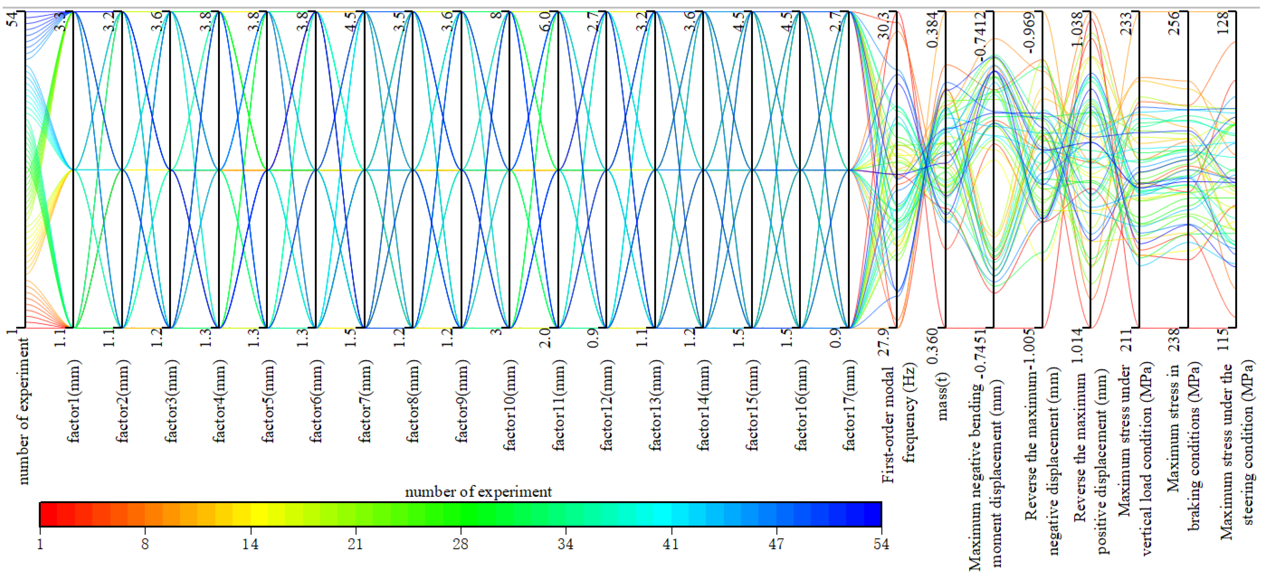
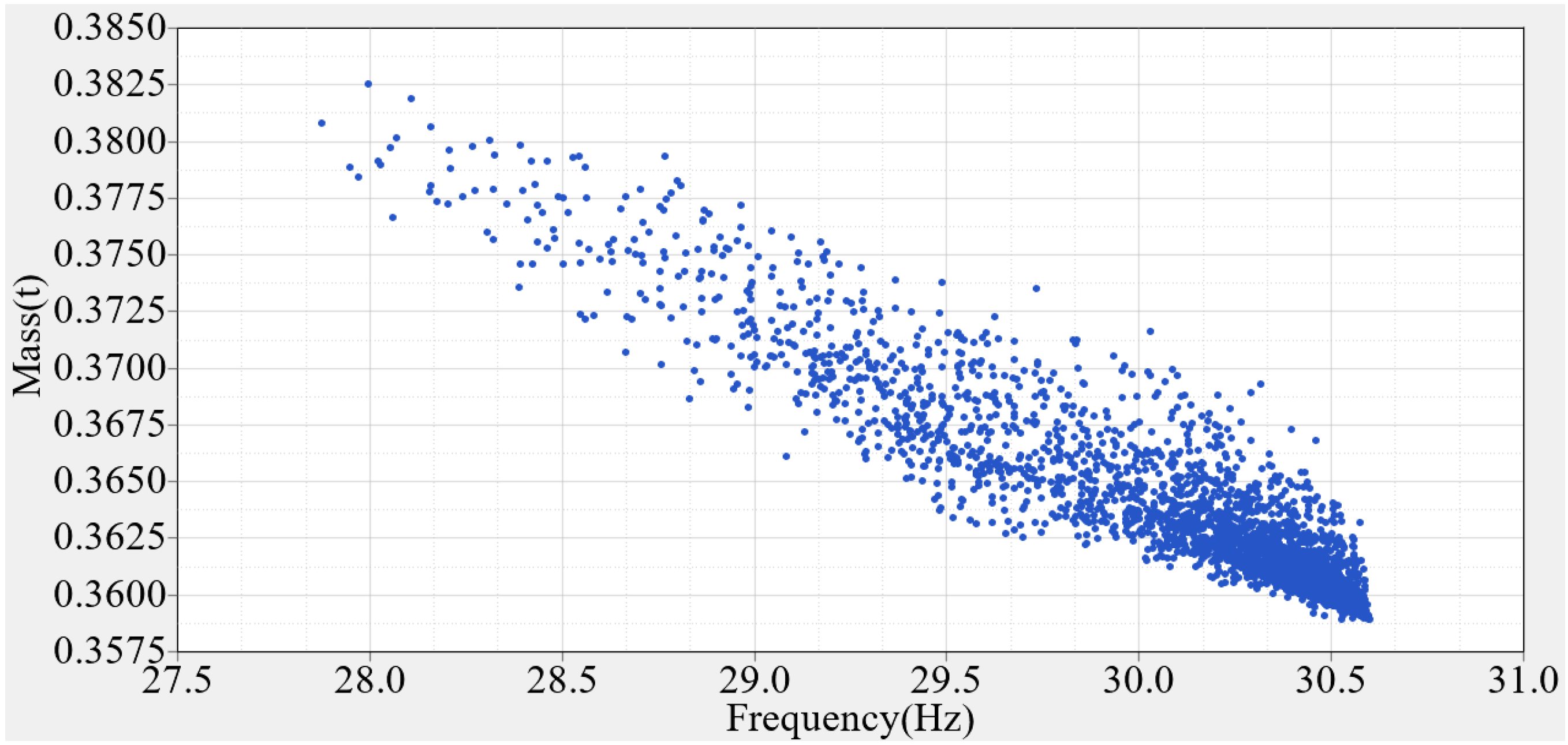
The Taguchi experiment uses the orthogonal array to study the interaction effect of different factors at various levels [31]. In Japan, 80% of the quality improvement methods are through the Taguchi experiment method. Through this method, the sample points are evenly distributed, and the number of experiments is greatly reduced compared with the full factor. The Taguchi experiment was conducted for 54 experiments with 17 factors and three levels (as shown in

Table 4. The design of the experiment.

Factor	3 Levels (mm)			Initial Value (mm)	Factor	3 Levels (mm)			Initial Value (mm)
1	1.1	2.2	3.3	2.2	10	1.2	2.4	3.6	2.4
2	1.05	2.1	3.15	2.1	11	2.5	5	7.5	5
3	1.2	2.4	3.6	2.4	12	2	4	6	4
4	1.25	2.5	3.75	2.5	13	0.9	1.8	2.7	1.8
5	1.25	2.5	3.75	2.5	14	1.05	2.1	3.15	2.1
6	1.25	2.5	3.75	2.5	15	1.5	3	4.5	3
7	1.5	3	4.5	3	16	1.5	3	4.5	3
8	1.2	2.4	3.6	2.4	17	0.9	1.8	2.7	1.8
9	1.15	2.3	3.45	2.3

). To analyze and understand the data from the Taguchi experiments, this paper uses parallel coordinate plots to describe the 54 experimental situations (as shown in Figure 17). The figure includes the complex cross-influences of 17 variables corresponding to eight responses. The 54 experiments are equivalent to 54 lines passing through these vertical coordinate axes, linking the changes in responses caused by the variables.

3. 

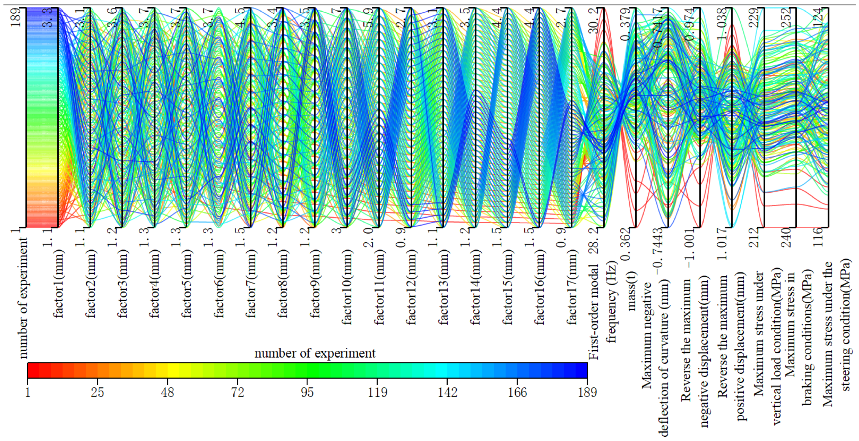
Hammersley sampling is a super-uniformly distributed sampling method [32], which is represented by converting the original data into decimal numbers in the interval [0, 1]. Compared with the Latin hypercube experiment, the uniformity of the Hammersley experiment is better in processing the 189 experimental data collection (as shown in Figure 18).

The 17 factors were sampled 189 times by the Hammersley experiment. In the Hamersley experiment, parallel coordinate plots were also drawn to observe the changes in variables and responses (as shown in Figure 19). In the parallel coordinate plots of the Hamersley experiment, there were 189 lines corresponding to 189 experiments. The parallel coordinate plots were used to correlate the changes in 17 variables and eight responses in the 189 experiments one by one.

5.2. Create the Response Surface Model

The response surface model is usually used to optimize engineering and predict response results [33]. Response results in the variable range are predicted by known variables and response data. Using a response surface model instead of a finite element model can reduce computational workload and improve work efficiency. The response surface polynomial constructed using the design variables is shown in Equation (4), and the second-order response surface polynomial is shown in Equation (5).

$$y=\tilde{y}(x)+\epsilon$$

(4)

$$\tilde{y}(x)={\beta }_0+{\displaystyle \sum _{i=1}^n{\beta }_i}{x}_i+{\displaystyle \sum _{i=1}^n{\beta }_{2i}}{x}_i^2+{\displaystyle \sum _{i=1}^{n-1}{\displaystyle \sum _{j=i+1}^n{\beta }_{ij}}{x}_i}{x}_j$$

(5)

In the formula: ε represents the error term, which follows a normal distribution N(0, σ²); $\tilde{y}(x)$—response function; β—constant term coefficient (regression coefficient; the coefficient number is (n + 1)(n + 2)/2); x—design variable; n—number of design variables.

In the creation of the response surface model of a constant, we need a suitable fitting method. Common fitting algorithms include LSM, MLS, Kriging method, and RBF (as shown in

Table 5. The characteristics of various fitting methods.

Fitting Method	Formula Expression	Nonlinear Problem	Noise Effect	Fitting Accuracy	Fitting Efficiency
LSM	√	×	√	Medium	Fastest
MLS	×	√	√	Good	Faster
Kriging	×	√	×	Best	Faster
RBF	×	√	×	Best	Faster

, the symbol √ represents “yes” and × represents “no”).

Through comparison, we found that LSM, MLS, and RBF have the best fitting effect, and the response surface model was constructed by these three fitting methods. Firstly, this paper uses the 189 experimental data from the Hamersley experiment as the training dataset, and the 54 experimental data from the Taguchi experiment as the test dataset. Then, the relative sensitivity is calculated for the 17 selected sheet metal thicknesses as the design variables, and the quality, first-order modal frequency, displacement in the stiffness analysis, and the maximum stress in the strength analysis are taken as the responses. Through this method, a response surface that represents the relationship between the variables and the responses can be constructed (as shown in Figure 20).

The constructed approximate model needs to be analyzed for its error, and the accuracy of the constructed approximate model is evaluated by using the maximum absolute error, root mean square error, and coefficient of determination (as shown in

Table 6. Error analysis.

Respond	Maximum Absolute Error			Root Mean Square Error			Coefficient of Determination (R2)
	A	B	C	A	B	C	A	B	C
a	3.01 × 10−7	8.23 × 10−7	7.57 × 10−7	1.21 × 10−7	3.53 × 10−7	2.88 × 10−7	1	1	1
b	0.0064	0.1269	0.0107	0.0020	0.0376	0.0028	0.999	0.995	0.999
c	6.20 × 10−5	2.43 × 10−4	7.50 × 10−5	2.52 × 10−5	9.11 × 10−5	2.79 × 10−5	0.998	0.992	0.998
d	3.78 × 10−4	0.0016	5.63 × 10−4	1.37 × 10−4	8.21 × 10−4	1.58 × 10−4	0.999	0.983	0.998
e	2.85 × 10−4	8.85 × 10−4	3.12 × 10−4	1.02 × 10−4	4.57 × 10−4	1.21 × 10−4	0.999	0.993	0.999
f	0.7984	1.6467	0.9647	0.0871	0.4176	0.1037	0.999	0.989	0.998
g	9.09 × 10−13	0.0499	0.0226	3.17 × 10−13	0.0211	0.0057	1	0.999	0.999
h	1.85 × 10−13	0.1102	0.0313	5.24 × 10−14	0.0396	0.0097	1	0.999	0.999

Note: A—training set (Hamersley experimental data); B—test set (Taguchi experimental data); C—cross-validation; a—mass; b—first-order mode frequency; c—maximum negative-displacement in Z direction under bending condition; d—maximum negative-displacement in Z direction under torsion condition; e—maximum positive-displacement in Z direction under torsion condition; f—maximum vertical impact stress; g—maximum stress in braking condition; h—maximum stress in steering condition.

). The results show that the determination coefficients of the approximate model built by the response surface are all above 0.98, which proves that the response surface model has good accuracy.

6. Results of Model Optimization

The approximate model created based on the response surface is optimized, which consists of three parts: design variables, constraints, and optimization objectives (as shown in Formula (6)). The optimization objective can be single or multiple, through the use of an optimization algorithm to solve the objective. Commonly used optimization algorithms include the adaptive response surface method (ARSM) [34], GA, and sequential quadratic programming method (SQP) [35], etc.

$$\begin{array}{lll}\mathrm{Objective}& \hspace{0.17em}Min\hspace{0.17em}f(x)\hspace{0.17em}or\hspace{0.17em}Max\hspace{0.17em}f(x),& d=1,2,3,\cdots ,n;\\ \mathrm{Restrict}& g_{\min }(x)\le g(x)\le g_{\max }(x),& v=1,2,3,\cdots ,n;\\ \mathrm{Design} \mathrm{variable}& x=[x_1,x_2,x_3,\cdots ,x_n]& \end{array}$$

(6)

We use ARSM, GA, and SQP to optimize the solution with the objective of mass minimization, take the first-order mode frequency, the maximum displacement in stiffness analysis, and the maximum stress in strength analysis as constraints, and obtain the iterative procedure and results of the three algorithms (where the population size and the number of iterations are shown in Figure 2, Figure 21, and Figure 22. The mutation probability is set at 0.01). For ARSM, the basic idea is to add a penalty term to the original objective function. When the solution violates the constraints, the penalty term will increase a large value to the objective function, putting the solution that violates the constraints at a disadvantage during the optimization process, thereby guiding the algorithm to search in the direction that satisfies the constraints. For GA, the constraint conditions are transformed into penalty functions and added to the objective function (fitness function). When an individual violates the constraint conditions, corresponding penalties are given based on the degree of violation to ensure that the optimal solution is within the constraints. In the selection operation, individuals that satisfy the constraint conditions are given priority. For individuals that do not satisfy the constraint conditions, a comprehensive assessment can be conducted based on their degree of constraint violation and fitness value to determine whether they are selected. For SQR, the principle is to convert the constraint conditions into penalty terms and add them to the objective function. When the solution violates the constraint conditions, the penalty terms will increase the value of the objective function, thereby preventing the violating solution from having an advantage in the optimization process and guiding the algorithm to search in the direction that satisfies the constraint conditions.

The iterative procedure regarding the quality is shown in Figure 21, the substitution procedure for the first-order mode frequencies is shown in Figure 22, and the optimization scheme for the three optimization algorithms is shown in Table 6.

The scatter plot (shown in Figure 23) shows that a large amount of data is concentrated in the places with higher frequency and lower mass. This proves that reducing the mass of these design variables can improve the first-order mode frequency. The response results of simulation experiments were compared and analyzed for these three optimization schemes (as shown in

Table 7. Comparison of the results of the three optimization schemes.

		The Initial Value (mm)	ARSM	GA	SQP
Design variable ID	1	2.2 mm	1.3 mm	1.1 mm	2.07 mm
	2	2.1 mm	1.25 mm	0.86 mm	1.95 mm
	3	2.4 mm	1.42 mm	0.96 mm	2.26 mm
	5	2.5 mm	1.51 mm	1 mm	2.43 mm
	6	2.5 mm	1.48 mm	1.27 mm	2.41 mm
	4	2.5 mm	1.48 mm	1.04 mm	2.23 mm
	7	3 mm	1.78 mm	1.35 mm	2.63 mm
	9	2.3 mm	1.36 mm	1.06 mm	1.9 mm
	8	2.4 mm	1.42 mm	0.97 mm	0.96 mm
	11	5 mm	3.75 mm	2.52 mm	4.84 mm
	12	4 mm	2.37 mm	1.6 mm	1.6 mm
	13	1.8 mm	1.07 mm	0.78 mm	1.14 mm
	14	2.1 mm	1.25 mm	0.95 mm	1.42 mm
	10	2.4 mm	1.42 mm	1.03 mm	2.21 mm
	15	3 mm	1.78 mm	1.43 mm	2.84 mm
	16	3 mm	1.78 mm	1.69 mm	2.81 mm
	17	1.8 mm	1.44 mm	2.64 mm	1.85 mm
Target	Mass (kg)	373.34	362.9	359	364.9
Constraint	First-order modal frequency (Hz)	29.067	30.097	30.563	30.332
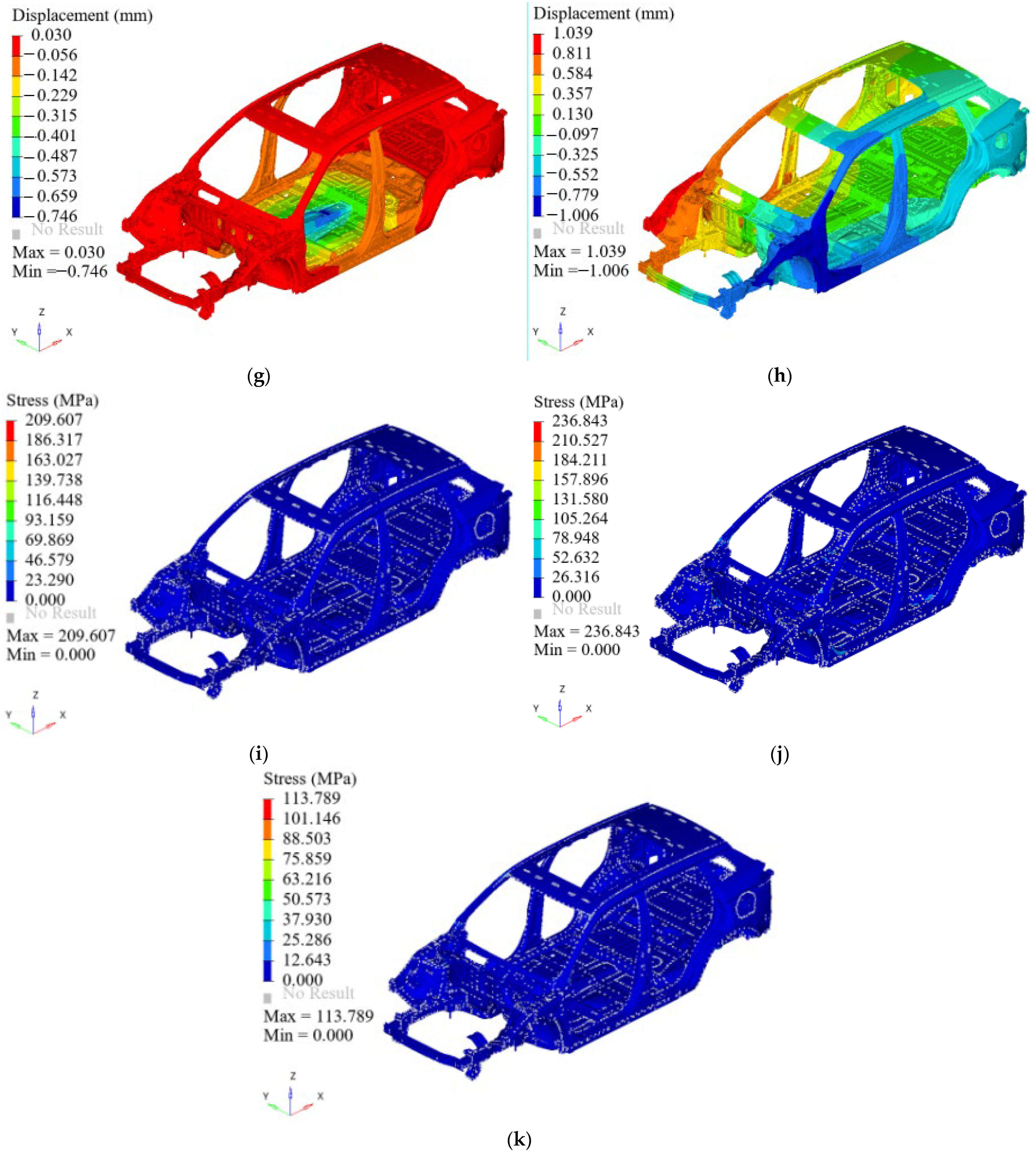
	Maximum negative-displacement in the Z-direction of bending stiffness (mm)	−0.742	−0.744	−0.7457	−0.743
	Maximum negative-displacement in the Z-direction of torsional stiffness (mm)	−0.983	−0.998	−1.006	−0.995
	Maximum positive-displacement of torsional stiffness in the Z direction (mm)	1.025	1.034	1.039	1.037
	Maximum stress under vertical load condition (MPa)	221.201	211.9	209.6	214.9
	Maximum stress under braking conditions (MPa)	246.92	239.9	236.8	242.4
	Maximum stress under steering conditions (MPa)	120.755	116	113.8	115.4
The average accuracy rate of the simulation results compared to the optimized results			99.98%	99.84%	99.97%
Quality variation (kg)			−10.44 kg	−14.34 kg	−8.44 kg

), and the optimization scheme with better effect and high accuracy was selected.

As shown in Table 7, all three optimization methods yield first-order modal frequencies within the range of 30 Hz to 31 Hz, and the average accuracy rate of the optimized results exceeded 99% compared to the simulation results ($\mathrm{accuracy}=(\left|b\right|-\left|\left|a\right|-\left|b\right|\right|)/\left|b\right|$, where a represents the response value calculated based on the optimization algorithm; b represents the response value obtained from the finite element simulation experiment). In the simulation results, the first-order mode frequency of the ARSM optimization method is 30.09 Hz, while the weight of the BIW has been reduced by 10.44 kg. The first-order mode frequency of the GA optimization method is 30.56 Hz, while the weight of the BIW has been reduced by 14.34 kg. The first-order mode frequency of the SQR optimization method is 30.33 Hz, and the weight of the BIW has been reduced by 8.44 kg. Although the maximum displacement of stiffness has slightly increased, the maximum stress of strength has decreased. In this paper, GA is used as the optimization algorithm, and Figure 24 shows the simulation results of the GA optimization calculation.

When calculating the stiffness of the optimized model, using the deformation of the observation point to calculate, the bending stiffness is 24,830.83 N/mm and the torsional stiffness is 22,041.63 N·m/°. Therefore, the optimization results using the genetic algorithm are shown in

Table 8. Results of GA optimization.

	Initial Value	Results of Optimization	Effect of Optimization	Percentage of Optimized Results
Total mass (kg)	373.34	359	−14.34	−3.84%
First-order mode frequency (Hz)	29.0677	30.56368	1.49598	5.14%
Bending stiffness (N/mm)	25,014.07	24,830.84	−183.23	−0.73%
Torsional stiffness (N·m/°)	22,410.39	22,041.63	−368.76	−1.64%
Maximum stress under vertical impact condition (MPa)	221.201	209.6	−11.601	−5.24%
Maximum stress under braking conditions (MPa)	246.92	236.8	−10.12	−4.09%
Maximum stress in steering condition (MPa)	120.755	113.8	−6.955	−5.75%

and Figure 25.

7. Conclusions

In this paper, the lightweight optimization design of the electric vehicle BIW is carried out based on the RSM-GA. In the optimization, the minimum mass optimization objective of the BIW, mode frequency, displacement, and maximum stress are taken as constraints. We selected 17 sheet metal parts as design variables through sensitivity analysis and relative sensitivity calculation. Then we obtained 243 sets of experimental data samples by 54 Taguchi experiments and 189 Hammersley experiments in the DOE methods. Next, we used the experimental data for response surface creation, and found that the accuracy of response surface fitting using LSR, MLSR, and RBF reached more than 98%. Finally, we use the optimization algorithm (ARSM, GA, and SQP) based on the response surface model to optimize the model solution. By comparison, we found that the optimization effect obtained by the genetic algorithm was better and the accuracy was high. After using the genetic algorithm, the total weight of BIW decreased by nearly 3.841%. Although the stiffness is slightly decreased, the modal frequencies of the first six orders are increased, and the maximum stress in the strength analysis is decreased, which meets the requirements of lightweight design.

However, this paper focuses on the lightweight optimization design of the vehicle body structure with an emphasis on stiffness and strength. However, merely focusing on these two aspects is far from sufficient. Vehicle body weight reduction is a complex part of system engineering that involves multiple disciplines and multiple performance indicators. It is necessary to shift from single-performance optimization to multi-disciplinary collaborative design, integrating material innovation, structural optimization, process upgrading, and AI technology, achieving a dynamic balance among stiffness, strength, fatigue, NVH, cost, and sustainability. Comprehensive consideration of the impact of light weighting on vehicle performance is also necessary. For example, in terms of collision safety, factors such as the vehicle’s energy absorption, collision force transmission path, and passenger protection effect are equally crucial. For instance, a seemingly structurally rigid and strong vehicle body may fail to effectively absorb and distribute collision energy during a collision, resulting in passengers experiencing excessive impact forces; or the transmission method of the collision force may be unreasonable, causing certain key components to bear excessive loads and suffer damage. Therefore, collision test research emphasizes the need to comprehensively consider multiple factors to achieve a lightweight design, breaking through the current limitations of only optimizing in terms of stiffness and strength; in the fatigue life domain, this includes improving the structural anti-fatigue performance through material optimization, etc. Vehicle body weight reduction achieves a balance in safety, durability, and energy efficiency through the collaborative optimization of materials, structure, and process, while meeting international standards such as ISO 12097-2, while enhancing dynamic performance, energy efficiency, and safety. In the next step of our work, we plan to conduct experimental verification on the optimized vehicle body structure (such as modal experiments and collision experiments), combine multi-disciplinary and multi-performance indicator coordinated optimization methods, build a parametric multi-objective optimization model, and then compare the experimental results with the simulation results to verify the feasibility of the proposed method in lightweight structure optimization design.

References

- Wenlong, S.; Xiaokai, C.; Lu, W. Analysis of energy saving and emission reduction of vehicles using light weight materials. Energy Procedia 2016, 88, 889–893. [Google Scholar] [CrossRef]
- Haugen, M.J.; Paoli, L.; Cullen, J.; Cebon, D.; Boies, A.M. A fork in the road: Which energy pathway offers the greatest energy efficiency and CO2 reduction potential for low-carbon vehicles? Appl. Energy 2021, 283, 116295. [Google Scholar] [CrossRef]
- Shi, T.; Si, S.; Chan, J.; Zhou, L. The carbon emission reduction effect of technological innovation on the transportation industry and its spatial heterogeneity: Evidence from China. Atmosphere 2021, 12, 1169. [Google Scholar] [CrossRef]
- Xie, G.; Fu, B.; Li, H.; Du, W.; Zhong, Y.; Wang, L.; Geng, H.; Zhang, J.; Si, L. A gradient-enhanced physics-informed neural networks method for the wave equation. Eng. Anal. Bound. Elem. 2024, 166, 105802. [Google Scholar] [CrossRef]
- Martin, N.P.; Bishop, J.D.; Boies, A.M. How well do we know the future of Co2 emissions? Projecting fleet emissions from light duty vehicle technology drivers. Environ. Sci. Technol. 2017, 51, 3093–3101. [Google Scholar] [CrossRef]
- Zhong, Y.; Xie, G.; Geng, H.; Hou, J.; Zhao, D.; He, W. Thermal analysis for plate structures using a transformation BEM based on complex poles. Comput. Math. Appl. 2024, 161, 32–42. [Google Scholar] [CrossRef]
- Ito, K.; Sallee, J.M. The economics of attribute-based regulation: Theory and evidence from fuel economy standards. Rev. Econ. Stat. 2018, 100, 319–336. [Google Scholar] [CrossRef]
- Park, J.H.; Kim, S.K.; Choi, B.I.; Lee, H.J.; Lee, Y.H.; Kim, J.S.; Kim, K.J. Optimal design of rear chassis components for lightweight automobile using design of experiment. Mater. Werkst. 2010, 41, 391–397. [Google Scholar] [CrossRef]
- Bastien, C.; Christensen, J.; Blundell, M.V.; Kurakins, J. Lightweight Body in White Design Using Topology-, Shape-and Size Optimisation. World Electr. Veh. J. 2012, 5, 137–148. [Google Scholar] [CrossRef]
- Kiani, M.; Shiozaki, H.; Motoyama, K. Simulation-based design optimisation to develop a lightweight body-in-white structure focusing on dynamic and static stiffness. Int. J. Veh. Des. 2015, 67, 219–236. [Google Scholar] [CrossRef]
- Duan, L.; Liu, X.; Xu, W.; Xu, D.; Shi, L.; Jiang, H. Thickness-based subdomian hybrid cellular automata algorithm for lightweight design of BIW under side collision. Appl. Math. Model. 2022, 102, 170–193. [Google Scholar] [CrossRef]
- Topac, M.M.; Karaca, M.; Aksoy, B.; Deryal, U.; Bilal, L. Lightweight design of a rear axle connection bracket for a heavy commercial vehicle by using topology optimisation: A case study. Mechanics 2020, 26, 64–72. [Google Scholar] [CrossRef]
- Hong, N.P.; Youngdoo, K.; Young, C. Lightweight design with metallic additively manufactured cellular structures. J. Comput. Des. Eng. 2022, 9, 155–167. [Google Scholar] [CrossRef]
- Xiong, F.; Wang, D.; Ma, Z.; Chen, S.; Lv, T.; Lu, F. Structure-material integrated multi-objective lightweight design of the front end structure of automobile body. Struct. Multidiscip. Optim. 2018, 57, 829–847. [Google Scholar] [CrossRef]
- Güler, T.; Demirci, E.; Yıldız, A.R.; Yavuz, U. Lightweight design of an automobile hinge component using glass fiber polyamide composites. Mater. Test. 2018, 60, 306–310. [Google Scholar] [CrossRef]
- Lu, S.; Ma, H.; Xin, L.; Zuo, W. Lightweight design of bus frames from multi-material topology optimization to cross-sectional size optimization. Eng. Optim. 2019, 51, 961–977. [Google Scholar] [CrossRef]
- Zhou, B.; Chen, J.; Zhang, Y.; Yang, S.; Lu, H. Optimization of laser spiral welding using Response surface methodology and genetic algorithms. J. Intell. Fuzzy Syst. 2023, 45, 2381–2392. [Google Scholar] [CrossRef]
- Liu, Z.; Li, H.; Zhu, P. Diversity enhanced particle swarm optimization algorithm and its application in vehicle lightweight design. J. Mech. Sci. Technol. 2019, 33, 695–709. [Google Scholar] [CrossRef]
- Liao, S.; Zhong, L.; Yi, L. Enhancing Vehicle Lightweight Design Process with Genetic Algorithm-Optimized BP Neural Network and Topology Optimization: A Comprehensive Study. Preprint 2024. [Google Scholar] [CrossRef]
- Chen, Z.; Jia, P.; Fan, Y.; Liu, Z. Parameter analysis and optimization of friction pendulum bearings in underground stations based on genetic algorithm. J. Earthq. Eng. 2022, 26, 7814–7831. [Google Scholar] [CrossRef]
- Alateyah, A.I.; El-Taybany, Y.; El-Sanabary, S.; El-Garaihy, W.H.; Kouta, H. Experimental investigation and optimization of turning polymers using RSM, GA, hybrid FFD-GA, and MOGA methods. Polymers 2022, 14, 3585. [Google Scholar] [CrossRef]
- Li, Q.; Tu, G.; Zhang, X.; Cheng, S.; Yang, T. Application of a back propagation neural network model based on genetic algorithm to in situ analysis of marine sediment cores by X-ray fluorescence core scanner. Appl. Radiat. Isot. 2022, 184, 110191. [Google Scholar] [CrossRef]
- Vukadinović, A.; Radosavljević, J.; Đorđević, A.; Protić, M.; Petrović, N. Multi-objective optimization of energy performance for a detached residential building with a sunspace using the NSGA-II genetic algorithm. Sol. Energy 2021, 224, 1426–1444. [Google Scholar] [CrossRef]
- Appadurai, M.; Raj, E.F. Finite element analysis of composite wind turbine blades. In Proceedings of the 2021 7th International Conference on Electrical Energy Systems (ICEES), Chennai, India, 11–13 February 2021; pp. 585–589. [Google Scholar] [CrossRef]
- Viano, D.C.; White, S.D. Seat strength in rear body block tests. Traffic Inj. Prev. 2016, 17, 502–507. [Google Scholar] [CrossRef]
- Yoon, D.S.; Kim, G.W.; Choi, S.B. Response time of magnetorheological dampers to current inputs in a semi-active suspension system: Modeling, control and sensitivity analysis. Mech. Syst. Signal Process. 2021, 146, 106999. [Google Scholar] [CrossRef]
- Panaro, D.B.; Frunzo, L.; Mattei, M.R.; Luongo, V.; Esposito, G. Calibration, validation and sensitivity analysis of a surface-based ADM1 model. Ecol. Model. 2021, 460, 109726. [Google Scholar] [CrossRef]
- Owais, M.; Moussa, G.S. Global sensitivity analysis for studying hot-mix asphalt dynamic modulus parameters. Constr. Build. Mater. 2024, 413, 134775. [Google Scholar] [CrossRef]
- Idriss, L.K.; Owais, M. Global sensitivity analysis for seismic performance of shear wall with high-strength steel bars and recycled aggregate concrete. Constr. Build. Mater. 2024, 411, 134498. [Google Scholar] [CrossRef]
- Politis, S.N.; Colombo, P.; Colombo, G.; Rekkas, D.M. Design of experiments (DoE) in pharmaceutical development. Drug Dev. Ind. Pharm. 2017, 43, 889–901. [Google Scholar] [CrossRef]
- Patel, N.S.; Parihar, P.L.; Makwana, J.S. Parametric optimization to improve the machining process by using Taguchi method: A review. Mater. Today Proc. 2021, 47, 2709–2714. [Google Scholar] [CrossRef]
- Li, Q.; Zhao, N. Probabilistic power flow calculation based on importance-Hammersley sampling with Eigen-decomposition. Int. J. Electr. Power Energy Syst. 2021, 130, 106947. [Google Scholar] [CrossRef]
- Chelladurai, S.J.; Murugan, K.; Ray, A.P.; Upadhyaya, M.; Narasimharaj, V.; Gnanasekaran, S. Optimization of process parameters using response surface methodology: A review. Mater. Today Proc. 2021, 37, 1301–1304. [Google Scholar] [CrossRef]
- Long, T.; Wu, D.; Guo, X.; Wang, G.G.; Liu, L. Efficient adaptive response surface method using intelligent space exploration strategy. Struct. Multidiscip. Optim. 2015, 51, 1335–1362. [Google Scholar] [CrossRef]
- Lin, X.; Wang, Z.; Zeng, S.; Huang, W.; Li, X. Real-time optimization strategy by using sequence quadratic programming with multivariate nonlinear regression for a fuel cell electric vehicle. Int. J. Hydrogen Energy 2021, 46, 13240–13251. [Google Scholar] [CrossRef]