Autonomous Parking Path Planning Method for Intelligent Vehicles Based on Improved RRT Algorithm

Abstract

Autonomous valet parking technology refers to a vehicle’s use of onboard sensors and line-controlled chassis to carry out a fully automatic valet parking function, which can greatly improve the driver’s experience. This study focuses on autonomous parking, employing environmental modeling and vehicle kinematics models. Innovatively applying the PSBi-RRT algorithm to path planning in autonomous parking systems constitutes this research’s contribution to this field. Firstly, the environment is modelled by the raster method; then, the PSBi-RRT algorithm is used for path planning, and a B-spline curve is used for path optimization. Speed and acceleration are smoothed at the same time, and finally, a smooth and obstacle-avoiding path planning scheme is obtained. The results show that an autonomous parking system based on the PSBi-RRT algorithm performs path planning from the vehicle to the parking space. Compared to RRT and Bi-RRT, PSBi-RRT generates shorter planning paths, smoother heading angle changes, shorter planning times, fewer nodes, and higher success rates. This research provides theoretical support for the development of autonomous parking technology.

1. Introduction

The increasing number of vehicles, coupled with the growing demand for mobility and the limited capacity of road infrastructure, has led to significant traffic and environmental challenges. The deployment of autonomous vehicles is expected to substantially alleviate traffic congestion, reduce fuel consumption, and lower transportation-related emissions [1].

Autonomous parking, as a critical component of advanced driver-assistance systems, eliminates the need for drivers to search for parking spaces and manually park, thereby enhancing both safety and efficiency during the parking process [2]. Currently, automated parking in autonomous driving is limited to scenarios where parking spaces are identifiable, and fully autonomous parking from the entrance of a parking facility to the parking spot without human intervention has yet to be commercialized. This end-to-end autonomous parking capability, requiring no human involvement, is an essential aspect of fully autonomous driving and holds significant research value [3,4].

Presently, path planning methods for autonomous parking primarily include curve interpolation, search-based algorithms, sampling-based techniques, and machine learning approaches [5]. These methods aim to optimize the parking trajectory and ensure seamless navigation within constrained environments.

The Rapidly-Exploring Random Tree (RRT) series of algorithms represents a classic sampling-based approach. Initially proposed by LaValle [6], RRT generates sample points in a Monte Carlo manner, but the polygonal lines connecting nodes are unsuitable for the motion paths of Ackermann-steering vehicles. Dong et al. [7] improved the baseline RRT by introducing reverse RRT tree growth and utilizing Reeds–Shepp curves to directly connect branches, along with RRT seed biasing, demonstrating that the algorithm remains complete and feasible under these modifications. Wang et al. [8] optimized the target point selection process in RRT* and refined the parent node selection procedure, incorporating Dubins curves for constraints. Wang [9] combined nonlinear optimization with an enhanced RRT* algorithm and Reeds–Shepp curves to improve path planning efficiency and address the limitation of discontinuous curvature in paths. Jhang et al. [10] employed an optimized Bidirectional RRT* (Bi-RRT*), enabling the proposed motion planner to navigate complex environments with obstacles and narrow spaces. In subsequent research [11], they revised the Bi-RRT* framework, proposing an efficient human-like motion planning method based on Reeds–Shepp curves, which generated human-like paths with high trajectory quality and consistency in parking scenarios. Meng et al. [12] introduced a speed-limited path planning algorithm, Kinodynamic Safety-optimal RRT* (KS-RRT*), which achieves near time-optimal paths through a rewiring procedure, as opposed to the distance-optimal paths in the original RRT*. Kim et al. [13] replaced the parking target in RRT with a set of backward parking paths (target tree), proposing the TargetTree-RRT* algorithm for complex environments and resulting in more accurate parking, faster generation of continuous curvature paths, and higher success rates. Wang et al. [14] combined the rapid search mechanism of RRT* with the positive feedback advantages of the ant colony algorithm, enhancing convergence speed and global search capabilities. Ma et al. [15] proposed a novel Probabilistic Smooth Bidirectional RRT (PSBi-RRT) for robotic path planning, incorporating a goal-biased strategy for sampling point selection and a node correction mechanism to adjust node coordinates, thereby reducing collision probabilities in cluttered environments. In addition, Wang et al. [16] proposed a GMR-RRT* hybrid path algorithm based on Gaussian mixture regression (GMR) and RRT*, which can learn navigation behavior from human demonstrations. The algorithm uses the probability density distribution of human trajectories generated by GMR to guide RRT* sampling, thereby quickly generating high-quality feasible paths. Ganesan et al. [17] proposed Hybrid-RRT*, which simultaneously uses uniform and non-uniform sampling, and compared it with RRT*, Informed RRT*, and RRT*-N. The experimental results show that Hybrid-RRT* is superior to the baseline algorithms in terms of convergence speed, success rate, number of nodes, path length, and planning time.

Bidirectional Rapidly-Exploring Random Trees (Bi-RRTs) have been widely applied in path planning and have demonstrated the capability to generate optimal paths for indoor robots. However, the quality of the initial solution is not guaranteed, and the convergence rate to the optimal solution is relatively slow. To address these limitations, this study proposes a novel bidirectional path planning algorithm, termed Probabilistic Smooth Bidirectional Random Tree (PSBi-RRT), for autonomous valet parking path planning. Initially, the environment is modeled using a grid-based approach, and a vehicle kinematics model is constructed. Based on the Ackermann steering principle, a four-wheel vehicle’s steering is simplified into a two-wheel model, and the kinematic model is established to determine the positions of all four wheels. Obstacle avoidance models for three common parking scenarios are defined. Subsequently, a vehicle path planning framework based on the PSBi-RRT algorithm is designed, incorporating B-spline curves for path optimization. Finally, simulations are conducted to validate the proposed method. The results demonstrate that the proposed approach successfully generates smooth and collision-free paths, effectively guiding the vehicle to the target parking space.

2. Environmental Modeling and Vehicle Kinematics Modeling

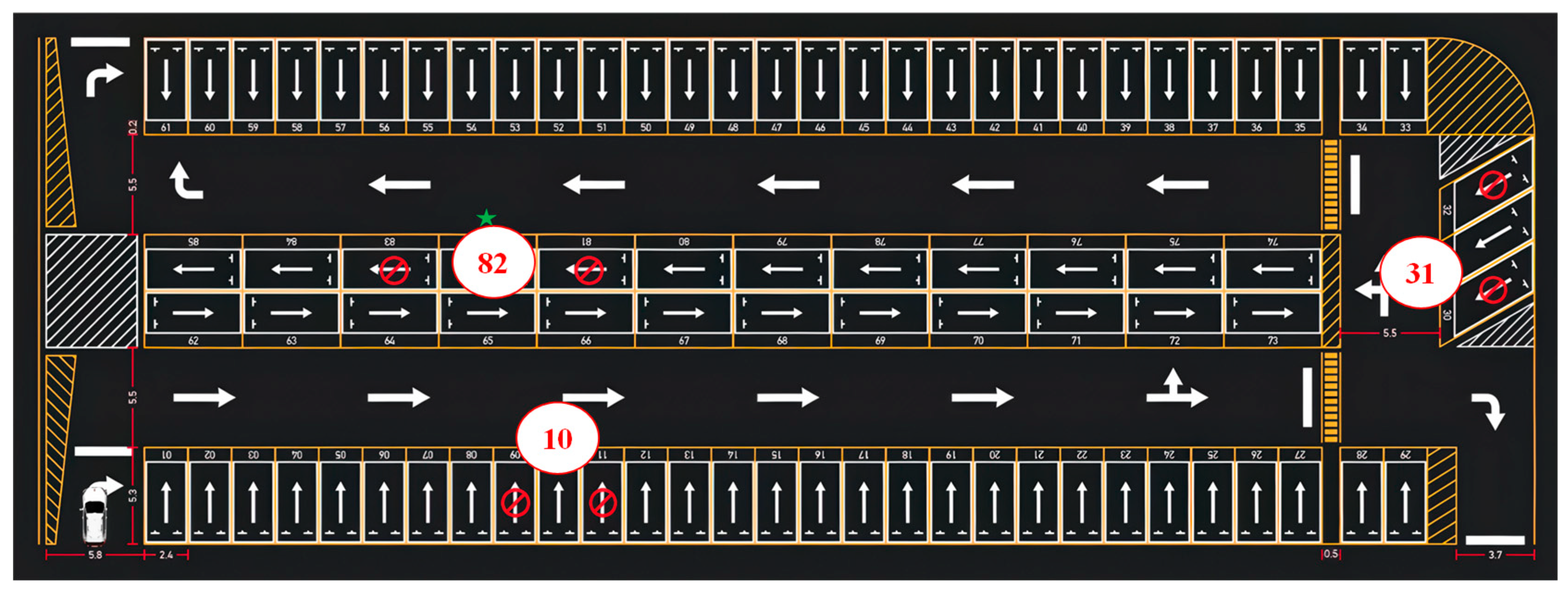
2.1. Environmental Modeling

Environment modeling refers to the mathematical representation of the parking environment required for autonomous parking path planning, enabling the generation of feasible and collision-free paths. In this study, a grid-based approach is adopted to construct the map model [18].

The following rules are established for constructing the environment using the grid-based method:

• A square grid is selected, with each grid cell having a side length of 0.1 m.
• In cases where obstacles with curved boundaries do not fully occupy a grid cell, the obstacles are expanded outward by one grid cell to ensure comprehensive coverage and accurate representation. This expansion is illustrated in Figure 1.

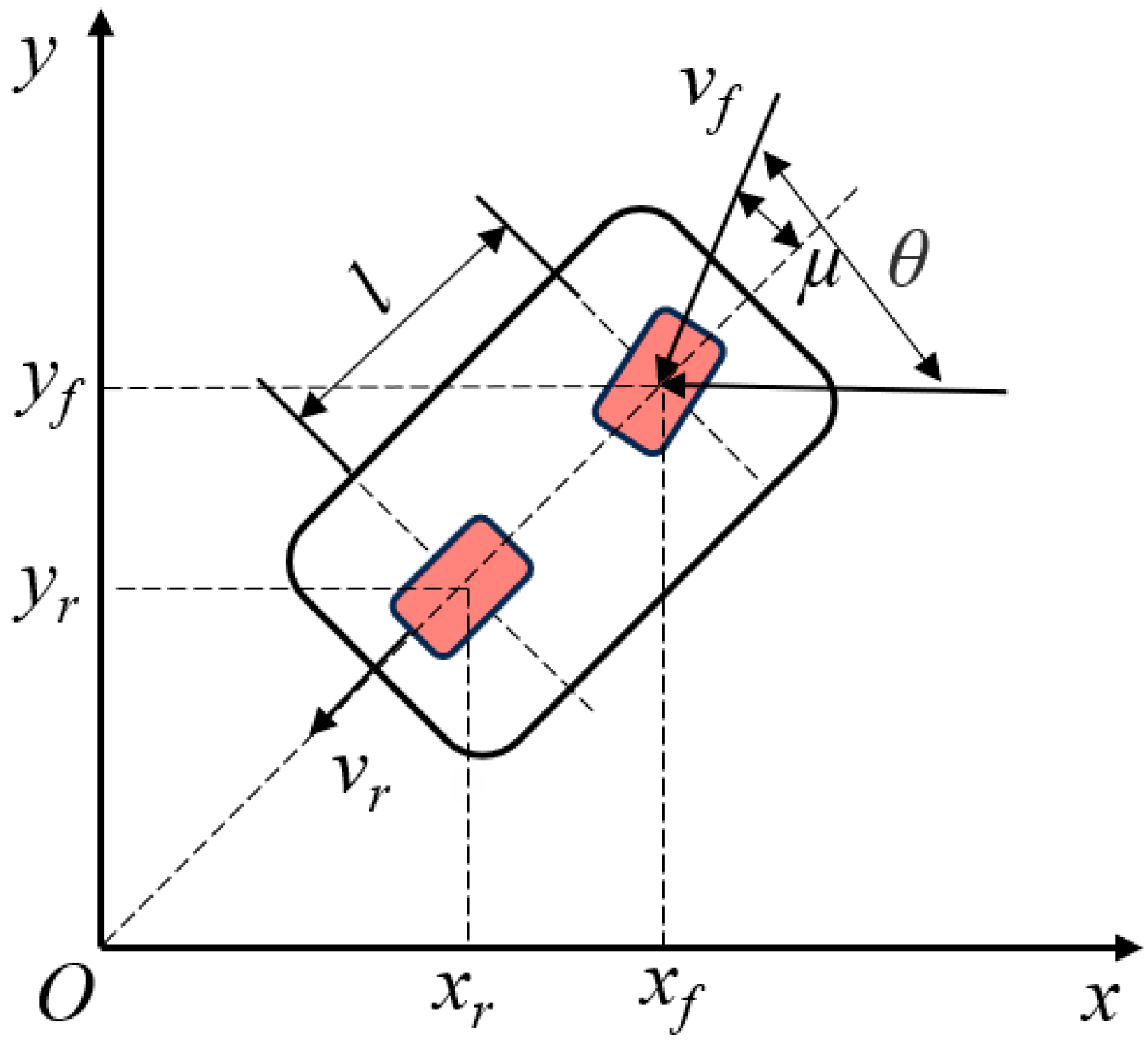
2.2. Vehicle Kinematics Modelling

By applying the Ackermann steering principle, the front and rear wheels of the vehicle are simplified into an equivalent two-wheel model [19], as illustrated in Figure 2. The kinematic model of the vehicle is established as follows: The coordinates of the rear axle center point are denoted as (x_r, y_r), and its velocity is v_r. The coordinates of the front axle center point are (x_f, y_f), with a velocity of v_f. The vehicle’s heading angle, defined as the angle between the velocity vector of the vehicle’s center of mass and the x-axis of the global coordinate system, is represented by θ. The steering angle of the front wheels relative to the x-axis of the vehicle’s body coordinate system is denoted as μ, which corresponds to the equivalent front wheel steering angle of the vehicle.

According to the Ackermann steering principle, in order to simplify calculations and ensure the feasibility of path planning, this study adopts an equivalent two-wheel kinematics model to describe the vehicle’s motion in the plane. Specifically, the rear axle’s center point velocity v_r and the front wheel’s angle μ determine the time-varying position (x_r, y_r) and heading angle θ of the vehicle in the plane through the classical non-complete constraint relationship. The model does not need to consider side-slip, and the body can be approximated as a left–right symmetric rectangle assuming that there is no external interference during vehicle travel. Among them, the change law of the rear axle’s center point coordinates with time obeys the following generalized differential equation:

$$\left[\begin{array}{l}{\dot{x}}_r\hfill \\ {\dot{y}}_r\hfill \\ \omega \hfill \end{array}\right]=\left[\begin{array}{c}\begin{array}{c}\cos \theta \\ \sin \theta \end{array}\\ {\displaystyle \frac{\tan \mu }{l}}\end{array}\right]v_r$$

(1)

Here, the inputs are the rear axle’s center velocity v_r and the front axle’s steering angle µ, while the outputs are the coordinates of the rear axle’s center (x_r, y_r) and the vehicle’s heading angle θ. This expression has been maturely derived in several papers, and the relevant complete derivation process is omitted to keep the text concise. Given the vehicle’s velocity and steering angle at any moment, the next state during parking can be predicted. However, since Equation (2) does not account for collisions with the surrounding environment, the vehicle’s body must be approximated as a rectangle to determine the motion constraints [20]. As shown in Figure 3, l represents the wheelbase (distance between the front and rear axles), l_r is the distance from the rear axle to the rear end of the vehicle, and l_f is the distance from the front axle to the front end of the vehicle. These parameters are used to define the vehicle’s physical boundaries and ensure collision-free motion during parking maneuvers.

The four corners of the rectangular vehicle body are designated as points A, B, C, and D. Based on the geometric relationships, the coordinates of these points can be calculated as follows:

Coordinates of point A:

$$\left\{\begin{array}{l}{x}_A=x_r+\left(l+l_f\right)\cos \theta -0.5W\sin \theta \hfill \\ y_A=y_r+\left(l+l_f\right)\sin \theta +0.5W\cos \theta \hfill \end{array}\right.$$

(2)

Coordinates of point B:

$$\left\{\begin{array}{l}{x}_B=x_r+\left(l+l_f\right)\cos \theta +0.5W\sin \theta \hfill \\ y_s=y_r+\left(l+l_f\right)\sin \theta -0.5W\cos \theta \hfill \end{array}\right.$$

(3)

Coordinates of point C:

$$\left\{\begin{array}{l}{x}_c=x_r-l_r\cos \theta -0.5W\sin \theta \hfill \\ y_c=y_r-l_r\sin \theta +0.5W\cos \theta \hfill \end{array}\right.$$

(4)

Coordinates of point D:

$$\left\{\begin{array}{l}{x}_D=x_r-l_r\cos \theta +0.5W\sin \theta \hfill \\ y_D=y_r-l_r\sin \theta -0.5W\cos \theta \hfill \end{array}\right.$$

(5)

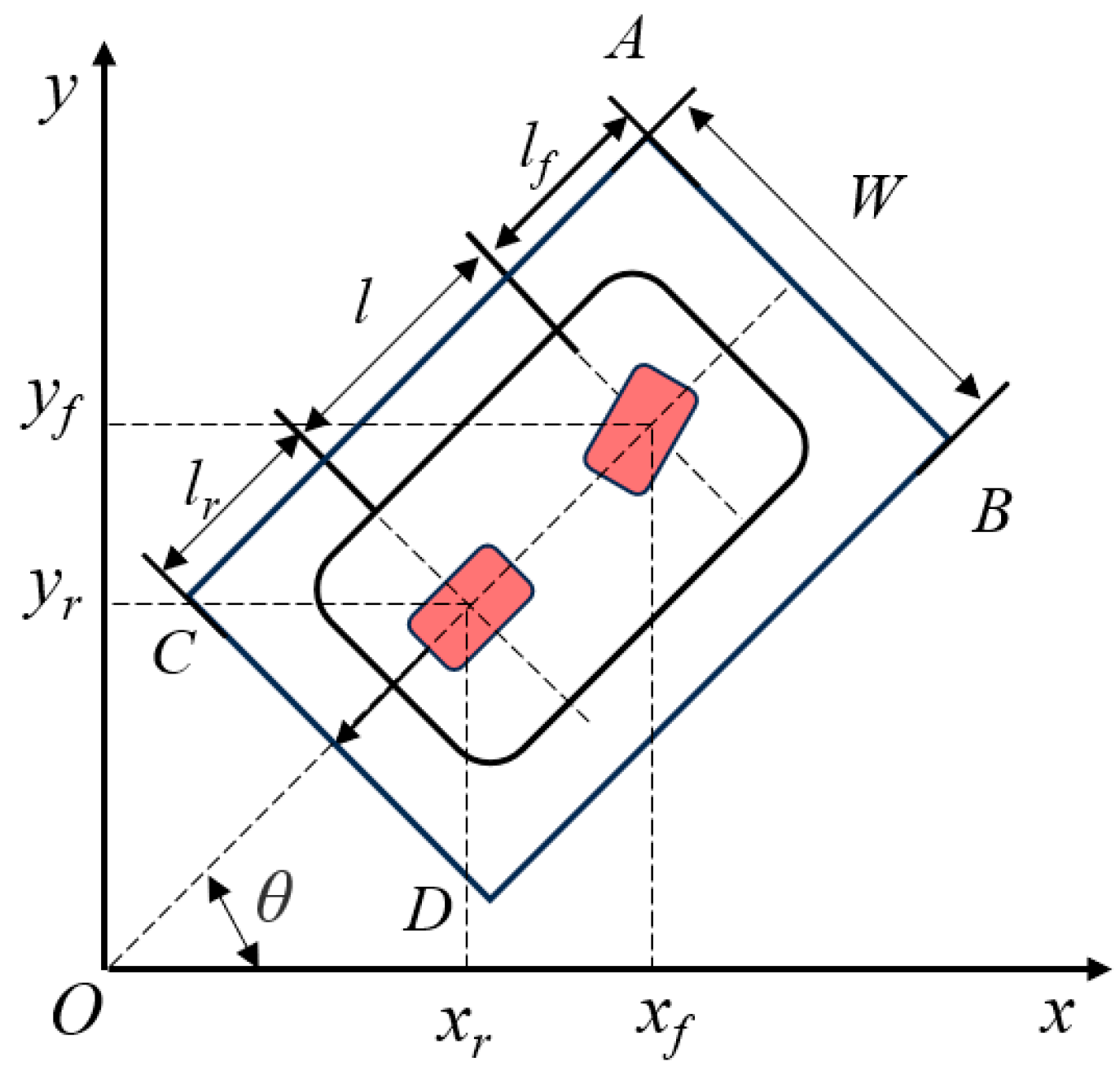
2.3. Parking Obstacle Avoidance Constraints

This section introduces the mathematical model for obstacle avoidance constraints in autonomous parking planning, providing theoretical support for the research and application of autonomous parking technology. The subsection begins by establishing obstacle avoidance constraints for three parking scenarios: vertical, parallel, and angled parking [4].

It is assumed that the vehicle moves on a two-dimensional plane, and the parking space is represented as a rectangular area. The vehicle’s initial position is denoted as point P₀ (x₀, y₀), and the target position is point P_t (x_t, y_t). The vehicle has a length l and a width w. During motion, the vehicle must avoid obstacles within the parking space, which are assumed to be known in terms of their position and shape and are represented as polygons. This study considers three parking scenarios: vertical parking, parallel parking, and angled parking. Since the obstacle avoidance constraint models for these scenarios are largely similar, the vertical parking case is elaborated in detail. In the vertical parking scenario, the vehicle is required to park perpendicular to the parking space. The parking space has a length L and a width W, with its center point denoted as P_c (x_c, y_c). The vehicle’s orientation is assumed to be 0 degrees, meaning that the vehicle’s front is aligned with the positive x-axis [21].

First, the vehicle’s parking position and orientation are determined. Let the parking position be denoted as P_p (x_p, y_p) and the orientation as θ degrees. The optimal parking position P_p and orientation θ are determined by minimizing the distance between the parking position and the target position. This can be formulated as an optimization problem:

$$\begin{array}{l}\begin{array}{cc}{\min }_{P_p,\theta }& \left|\right|P_p-P_t|{|}_2\end{array}\\ s.t.\left\{\begin{array}{l}{P}_p=P_c+(L/2+l/2)\cos (\theta )\widehat{i}+\\ (W/2+w/2)\sin (\theta )\widehat{j}\\ \theta \in [0,180]\end{array}\right.\end{array}$$

(6)

Here, $\left|\right|\cdot |{|}_2$ represents the Euclidean distance, while $\widehat{i}$ and $\widehat{j}$ denote the unit vectors in the x and y directions, respectively.

Then, the obstacles to be avoided by the vehicle during its movement are identified. Assuming that the vertex coordinates of the obstacle are P_i (x_i, y_i) i = 1, 2, …, n, the obstacle is represented as a polygon, i.e.,

$$\mathcal{O}={\{(x_i,y_i)\}}_{i=1}^n$$

(7)

To prevent collisions between the vehicle and obstacles, the vehicle’s outline is represented as a rectangle, and whether the rectangle intersects with the obstacles is determined. Specifically, the vehicle’s outline is represented by four vertices P₁, P₂, P₃, and P₄, where P₁ and P₂ denote the vertices on both sides of the front of the vehicle, and P₃ and P₄ denote the vertices on both sides of the rear of the vehicle. Then, it is checked whether any of the four edges intersect with the obstacles, i.e.,

$$\begin{array}{l}\{(P_1,P_2),(P_2,P_3),(P_3,P_4),(P_4,P_1)\}\cap \mathcal{O}\ne \varnothing \\ \Rightarrow \exists i,j,k\in \{1,2,\dots ,n\} \mathrm{s}.\mathrm{t}. (P_i,P_j),\\ (P_j,P_k) \mathrm{intersect} \mathrm{with} \mathcal{O}\end{array}$$

(8)

Here, (P_i, P_j) represents the line segment from point P_i to point P_j.

The obstacle avoidance constraints between the vehicle and the obstacles can be expressed as follows:

$$\{(P_i,P_j),(P_j,P_k)\}\cap \mathcal{O}=\varnothing , i,j,k\in \{1,2,\dots ,n\}$$

(9)

In summary, the obstacle avoidance constraints for autonomous parking planning can be formulated as a mathematical model, which is used to solve the optimization algorithm.

3. Vehicle Path Planning

The Probability Smoothing bidirectional RRT (PSBI-RRT) algorithm is a novel bidirectional path planning algorithm that addresses the limitations of the traditional RRT algorithm used in path planning and ensures the determination of an optimal solution. In this study, the PSBi-RRT algorithm is applied to the autonomous parking problem in parking lots for path planning, and B-spline curves are utilized to optimize the generated paths. The final result is a smooth and obstacle-free path planning solution.

The specific process of path planning begins with inputting the start and end points, followed by generating obstacles and expanding nodes. It is then checked whether the node lies within the target region. If it does lie within the target region, the optimal path is directly generated, and the resulting path curve is segmented. After applying B-spline optimization, collision detection is performed on the path. If a collision is detected, the parameters are adjusted to re-optimize the path until no collision occurs, and the final path curve is output. If the node is not within the target region, a random sampling point is generated and connected to the nearest node, after which a new node is added. The newly added node is connected, and collision detection is performed. If no collision occurs, the connection is established, forming a new spatial search tree. The process then returns to the initial step to check if the node is within the target region, and this cycle is repeated until the optimal path is found, as shown in Figure 4.

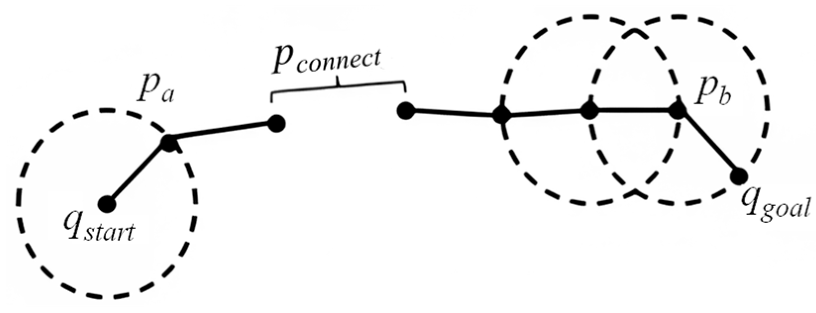
3.1. PSBi-RRT Algorithm

PSBi-RRT is a novel bidirectional path planning algorithm, termed Probabilistic Smooth Bi-RRT, that is designed to address the issues associated with the RRT algorithm [22,23,24], used in path planning, and used to determine the optimal solution. First, the algorithm narrows the sampling range to an ellipse and employs a dual-goal biasing strategy to sample within the ellipse. After sampling, a heuristic method is introduced to enable the sampling points to locate nearby nodes. This algorithm is applied for the first time in autonomous vehicle parking. In this study, the kinematic model of the parking vehicle is established based on the Ackermann steering principle and vehicle kinematic constraints to facilitate the implementation of this algorithm. Figure 5 illustrates the node sampling process of the Bi-RRT algorithm, showcasing the dual-tree connection process and the formation of the final planned path by P_a, P_b, and P_connect.

Compared to traditional RRT, which uniformly samples the entire feasible space each time, wasting a large number of samples, PSBi-RRT first constructs an elliptical region covering the root nodes of the two current search trees and samples within this ellipse while simultaneously biasing toward the starting point or endpoint with a certain probability, thereby greatly improving the relevance and efficiency of sampling. In terms of node expansion, traditional RRT only expands unidirectionally from the starting point, while PSBi-RRT uses bidirectional expansion, greatly accelerating the search speed. In terms of path smoothness, the trajectories generated by traditional RRT are often composed of multiple directly connected straight segments, resulting in numerous curvature changes that require specialized smoothing to accommodate the continuous turning requirements of vehicles. In contrast, PSBi-RRT, after completing connectivity, uses an internal probabilistic smoothing approach combined with B-spline curves for one-time optimization.

Node Expansion Approach: Sample the random point qrand; find the nearest node q_near to q_rand; generate a new node q_new along the geodesic from q_near to q_rand3 check if the new node collides with any rectangular obstacles; if not, add the new node to the spatial search tree; check if the path from q_near to q_new to observe whether it collides with any rectangular obstacles; if the path does not collide with obstacles, add q_new to the node; draw a path from q_near to q_new. This approach can automatically generate a feasible path given the start point, end point, and obstacle information and save it to a file. Among its main functions are defining obstacles and path planning parameters, generating an RRT tree, determining whether a node collides with an obstacle, and searching for the optimal path. The pseudocode of the Algorithm 1 is as follows.

Algorithm 1 PSBi-RRT

Input: Ta.V, Ta.E, Tb.V, Tb.E,Ta.V1 = Qstart, Tb.V1 = Qgoal   Output: Tree ← Ta ∪ Tb

1: initialize Tree = (V ← ,Qgoal; E ← ∅; map; ρ; N; I ← 0);

2: While i ≤ N do

3: Xf← Ellipticalization of samplingrange (X);

4: Qrand ← Dual-target bias strategy (Xf;Tree);

5:Qnear← Heuristic search nearby points (Tree,Qrana);

6: Qnew← Extension new nodes (Qnear,Qrand,ρ);

7: Qnew* ← Node correction (Qnew,Qnear);

8: if ObstacleFree (Ta.Qnear, Ta.Qnew) then

9:      Ta.V1 = Ta.V1 ∪ Ta. Qnew*;

10:      Ta.E1 = Ta.E1 ∪ (Ta. Qnear, Ta. Qnew*);

11: end if

12: if ObstacleFree (Tb.Qnear, Tb.Qnew) then

13:      Tb.V1 = Tb.V1 ∪ Tb. Qnew*;

14:      Tb.E1 = Tb.E1 ∪ (Tb. Qnear,Tb. Qnew*);

15: end if

16: if Ta. Qnew*= = Tb. Qnew* then

17:     Path = FillPath (TaTb);

18: else if Ta. Qnew*! = Tb. Qnew* then

19:     DirectConnection (Ta, Tb);

20:     Swap (Ta, Tb);

21:   end if

22:   Tree ← θ-cutmechanism (Ta ∪ Tb, Xf)

23: end while

In the above pseudocode, we first establish two search trees at the start and end points. In each iteration, we generate a random configuration point using “elliptical constraint sampling”. During sampling, we consider the bias along the start or end point direction while maintaining a uniform distribution within the overall elliptical region to balance global exploration. Next, for each tree, we first use the distance function to find the node in the current node set that is closest to the random point and then generate a new expansion node with a fixed step size and only add it to the search tree if there is no collision between the new node and its parent node, thereby ensuring the feasibility of the path. Additionally, we apply a simple heuristic adjustment to the newly expanded node to make it more inclined toward the opposite search tree, further reducing the risk of obstacles when the two trees meet. When the nodes expanded by the two trees are sufficiently close in Euclidean distance, the two trees are deemed to have “met,” at which point the connection function is called to merge the two subpaths into a complete feasible path and return it; if the connection is not completed within the predefined maximum iteration count, the algorithm stops and returns failure or the current best path. The entire process alternates and symmetrically expands the tree structures on both sides, combining elliptical constraints with dual-objective biases and a simple node correction strategy. This ensures path smoothness while effectively reducing unnecessary node expansion and computational overhead, thereby achieving efficient bidirectional path search.

3.2. Planning Models for B-Spline Curves

B-spline curves are a polynomial-based curve interpolation method that generates smooth curves through a series of control points. First, the points generated along the RRT path are used as control points to construct a B-spline curve. Next, the influence of obstacles on the path must be considered. This can be achieved by incorporating the positions of obstacles as constraints and optimizing the B-spline curve accordingly. A common optimization approach is to use nonlinear programming algorithms, where factors such as path smoothness, length, and distance from obstacles are treated as objective functions. This transforms the path planning problem into an optimization problem, and the optimal path is obtained by solving this problem. During the optimization process, weight coefficients can be adjusted to balance the importance of different objective functions, ensuring that the resulting path meets practical requirements. Finally, based on the optimized B-spline curve, a smooth and obstacle-free path planning solution is generated.

A nonlinear optimization model is used for path optimization, assuming that the control points on the path are P_i (x_i, y_i) and the B-spline curve of the path is C(u) = (x(u), y(u)), where u∈ [0,1]. Consider the effect of obstacles on the path, and assume that there are n obstacles, the location of the jth obstacle is (x^o_j, y^o_j), and the radius of the obstacle is r_j. In order to avoid the obstacles, the following constraints need to be satisfied:

• All points (x(u), y(u)) on the B-spline curve have distances from all obstacles greater than or equal to the obstacle radius r_j, i.e.,

$$\sqrt{{(x(u)-x_j^o)}^2+{(y(u)-y_j^o)}^2}\ge r_j,j=1,2,\cdots ,n$$

(10)

2.

The start and end points of the B-spline curve are P₁ and P_n, i.e.,

$$x(0)=x_1,y(0)=y_1,x(1)=x_n,y(1)=y_n$$

(11)

3.

The first-order derivative of the B-spline curve is continuous, i.e.,

$$\begin{array}{l}{\displaystyle \frac{dx(u)}{du}}{|}_{u=k}={\displaystyle \frac{dx(u)}{du}}{|}_{u=k+ϵ},\\ {\displaystyle \frac{dy(u)}{du}}{|}_{u=k}={\displaystyle \frac{dy(u)}{du}}{|}_{u=k+ϵ}\end{array}$$

(12)

where k = 1, 2, …, n − 1 is a small positive number.

In summary, the path planning problem can be transformed into the following nonlinear planning problem:

$$\begin{array}{l}{\min }_{C(u)}{\displaystyle \sum _{i=1}^{n-1}\sqrt{{(x_{i+1}-x_i)}^2+{(y_{i+1}-y_i)}^2}}+\\ \alpha {\displaystyle \sum _{j=1}^n\frac{1}{r_j}}{\displaystyle \sum _{i=1}^m\max }(0,r_j-\sqrt{{(x_i-x_j^o)}^2+{(y_i-y_j^o)}^2})\end{array}$$

(13)

where the first term is the length of the path, the second term is the cost of avoiding obstacles, α is the weighting factor, and m is the number of sampling points on the B-spline curve.

The constraints are as follows:

$$\left\{\begin{array}{l}\sqrt{{(x(u)-x_j^o)}^2+{(y(u)-y_j^o)}^2}\ge r_j,j=1,2,\cdots ,n,u\in [0,1]\\ x(0)=x_1,y(0)=y_1,x(1)=x_n,y(1)=y_n\\ {\displaystyle \frac{dx(u)}{du}}{|}_{u=k}={\displaystyle \frac{dx(u)}{du}}{|}_{u=k+ϵ},{\displaystyle \frac{dy(u)}{du}}{|}_{u=k}={\displaystyle \frac{dy(u)}{du}}{|}_{u=k+ϵ},\\ k=1,2,\cdots ,n-1\end{array}\right.$$

(14)

Obstacle avoidance constraints and vehicle dynamic constraints are introduced to ensure that the trajectory is both smooth and feasible. Obstacle constraints are implemented by uniformly sampling several points on the curve and detecting the minimum distance between these points and the obstacle boundaries to ensure that the trajectory maintains a safety margin throughout the entire path. If a section of the trajectory is too close to an obstacle, a penalty is applied during optimization to guide the control points toward a safer area. In terms of vehicle dynamic constraints, we considered factors such as maximum allowable turning curvature, speed, and acceleration. During optimization, the smoothness of the path is adjusted to reduce curvature peaks and improve trackability. If there is a tendency for curvature or acceleration to exceed limits in a local path, the optimization algorithm automatically fine-tunes the relevant control points to make the trajectory more suitable for actual execution. To balance different objectives, we set four optimization targets, path length, smoothness, safety distance, and dynamic constraints, and adjusted them using weighting factors. Through multiple experiments, we determined a set of empirical weighting parameters, 1, 5, 10, and 2, ensuring that the final trajectory is both smooth and reasonable while meeting obstacle avoidance and dynamic feasibility requirements. The problem can be solved using existing nonlinear programming algorithms to obtain the optimal B-spline curve and hence the optimal path planning scheme.

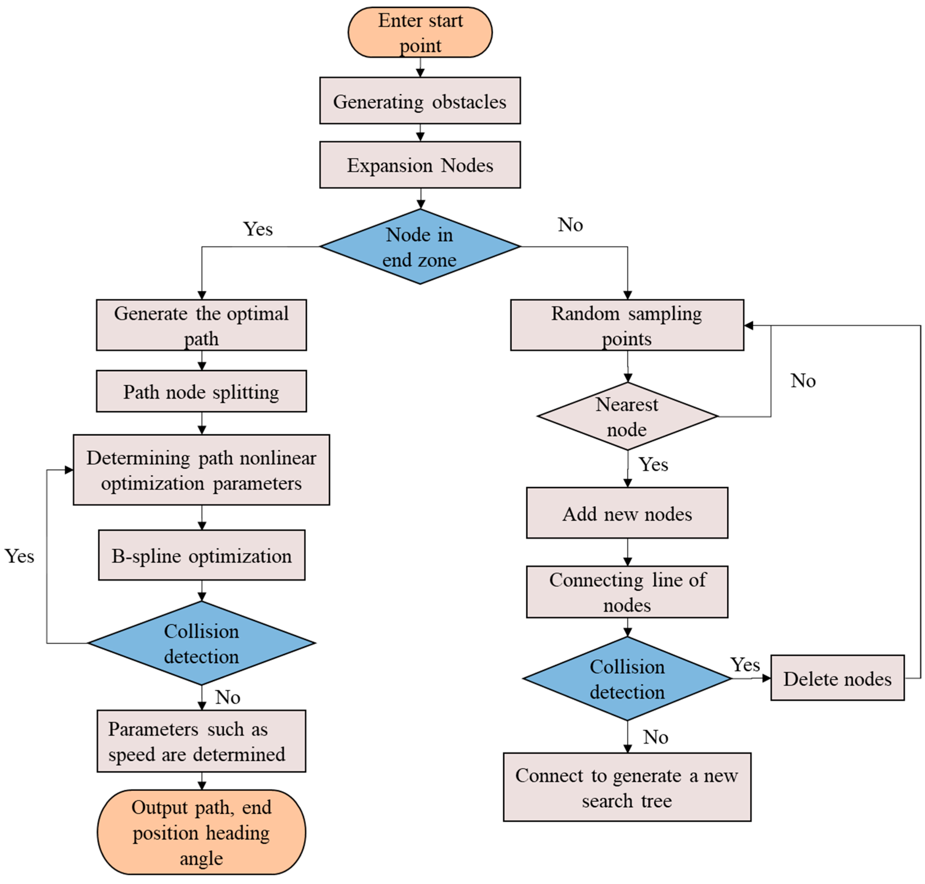
4. PSBi-RRT Algorithm Path Planning Implementation

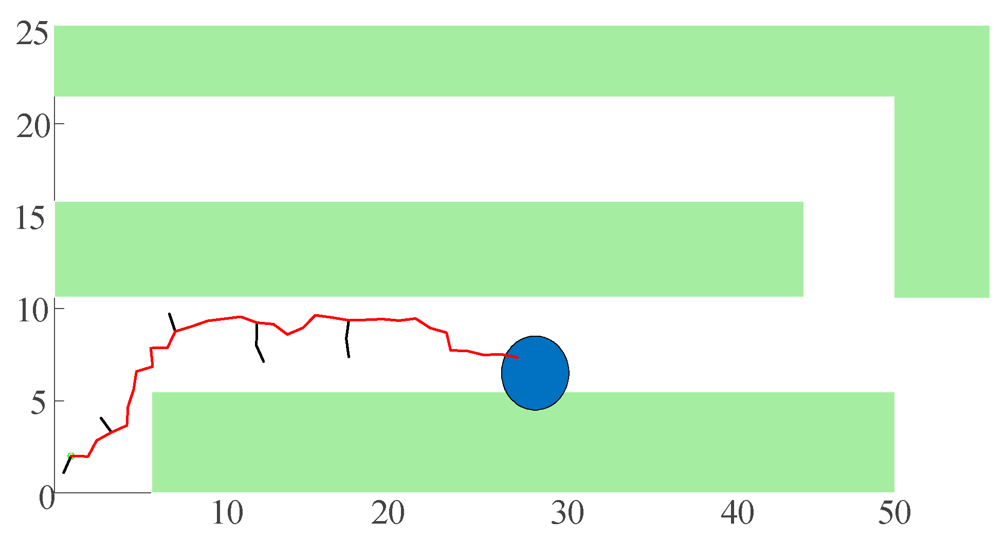
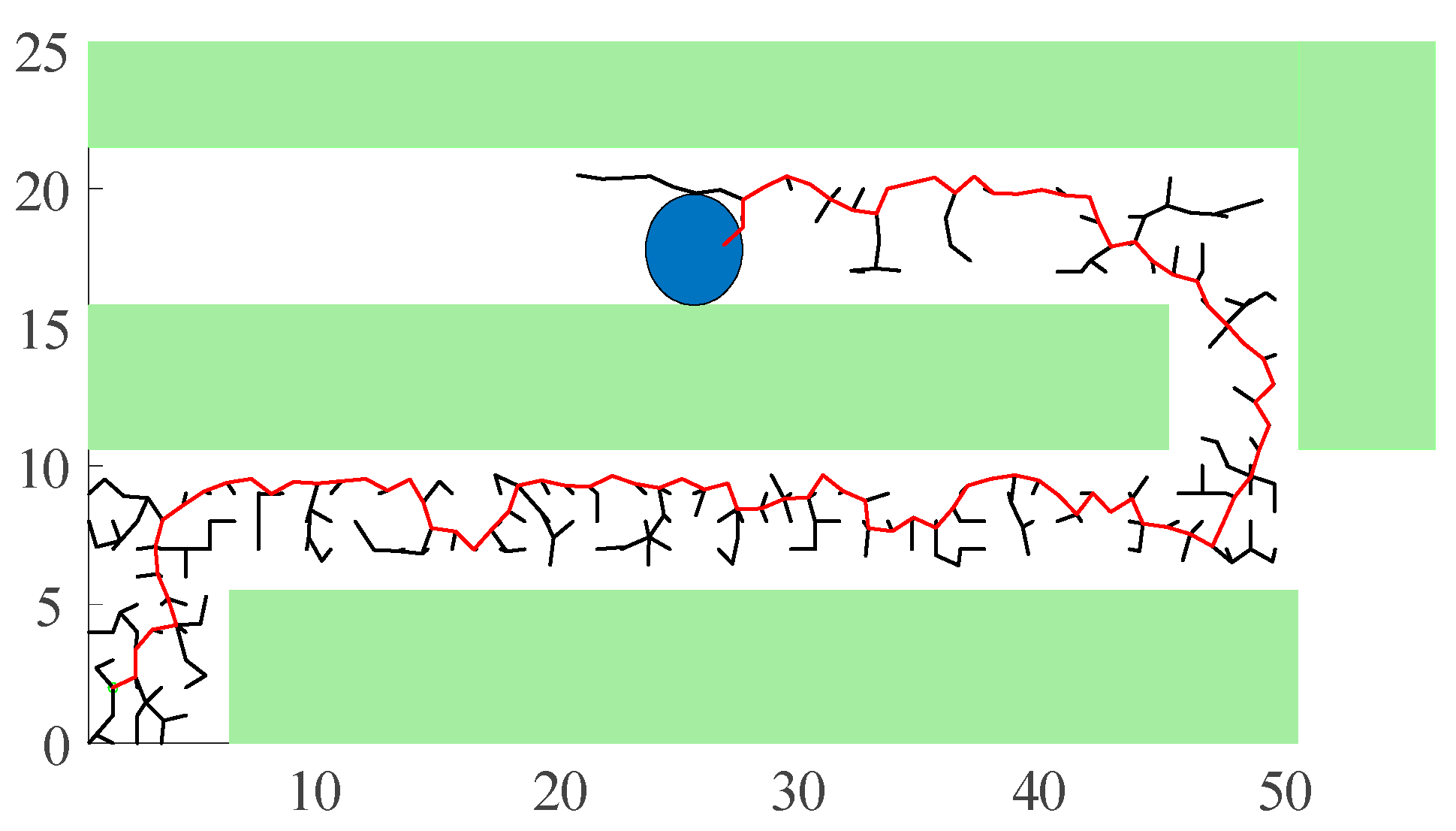
To systematically assess the performance and robustness of the PSBi-RRT algorithm under realistic conditions, the following numerical assumptions and simulation parameters are adopted.

The test scenario is defined as follows: The parking lot is 55.6 m long and 27 m wide. The vehicle body is treated as a rectangle with a length of 4.9 m and a width of 1.8 m. The wheelbase is 2.8 m, and the track width is 1.7 m. The maximum throttle acceleration is 3.0 m/s², the maximum deceleration is −6.0 m/s², and the jerk (rate of change of acceleration) should not exceed 20.0 m/s³. The steering wheel has a maximum rotation angle of 470°, with a steering ratio of 16:1 (16° of steering wheel rotation corresponds to 1° of front wheel rotation). The maximum steering wheel rotation speed is 400°/s. In addition, although this study mainly focuses on path planning based on kinematic and geometric constraints, in actual electric or hybrid vehicles, energy consumption and powertrain efficiency during trajectory execution must also be considered [25].

Figure 6 depicts the layout of a parking lot. The autonomous vehicle starts from its initial position with an initial velocity of zero and is required to park in one of the parking spaces. In the figure, yellow diagonal lines represent the partial walls of the parking lot, white diagonal areas indicate no-entry zones where the vehicle must avoid conflicts or collisions, and yellow horizontal lines denote speed bumps. The arrows within the parking spaces indicate the vehicle’s heading direction after parking. Arrows on the ground specify the direction in which the vehicle should travel, with no constraints on reversing during the parking process. Within 5 m before and after the yellow speed bumps, the vehicle’s speed must not exceed 10 km/h.

During the parking process, the duration should be as short as possible while ensuring safety. The forward speed should not exceed 20 km/h, and the reverse speed should not exceed 10 km/h. Within 5 m before and after speed bumps, the speed should not exceed 10 km/h. Both the trajectory and speed should be as smooth as possible. Here, the trajectory refers to the path of a specific point on the vehicle body, known as the control point. The control point is predetermined and is typically located on the vehicle’s longitudinal axis of symmetry (the vehicle body can be approximated as left–right symmetric). During motion, the position of the control point coincides with the trajectory point, and the velocity direction at the control point aligns with the direction angle of the trajectory point. In this study, the control point is assumed to be located at the center of the rear axle.

4.1. Path Planning

In order to evaluate the application of the algorithm in real parking lot scenarios, we chose three representative parking spaces: No. 10: perpendicular parking space; No. 82: parallel parking space; and No. 31: tilted parking space (with a tilt angle of 45°). These scenarios cover the most common parking operations and provide a comprehensive testbed for path planning. As shown in Figure 7. We combined the minimum turning radius of the vehicle (1.0 m) and the environmental grid resolution (0.1 m) to set the extension step size to 0.5 m. This step size ensures that each extension falls within the feasible space and does not “skip” narrow passages while avoiding the problems of excessive nodes and significantly increased computation time caused by too small a step size. Setting the maximum iteration count to 100,000 ensures a high search probability even in complex environments. r_goal = 2.0 m is chosen because each parking space is approximately 2.5 m wide. To ensure that the vehicle’s rear axle center fully enters the parking area, the target region is defined as a circular area with a radius of 2.0 m centered at the target point. Once a node in the search tree enters this circle, the path is considered to have reached the target, and the planning is successful. The detailed parameter settings are shown in

Table 1. Parameter settings.

goal_region_radius	numNodes	EPS	delta	Δt	vmax	w_max	amax	gamma_max
2	1,000,000	1	0.5	10 s	10 km/h	pi	2	pi

.

For vertical parking space #10, the end point of the vehicle’s path planning was set as a circular area with a radius of 2 at a point next to the space, path planning was started with the start point of the vehicle in the lower left corner, and the vehicle traveled along a collision-free path from the start point to the target area, maintaining a minimum turning radius and avoiding obstacles along the way. Critical waypoints are labeled to show smooth transitions for each turn segment, and the final result is shown in Figure 8.

For the 31st angled parking space (with a tilt angle of 45°), the endpoint of the vehicle’s path planning is set as a circular region with a radius of 2 centered at a point near the parking space. Starting from the initial position at the bottom-left corner, path planning is performed, and the final result is shown in Figure 9.

For the 82nd parallel parking space, the endpoint of the vehicle’s path planning is set as a circular region with a radius of 2 centered at a point near the parking space. Starting from the initial position at the bottom-left corner, path planning is performed, and the final result is shown in Figure 10.

In both the perpendicular and inclined parking scenarios in Figure 8 and Figure 9, the vehicle completes its turn and aligns itself with the parking space in one continuous curve, whereas in the parallel parking example in Figure 10, the trajectory exhibits a moderate U-turn. This is mainly due to the fact that parallel parking spaces have a larger lateral offset from the starting position, and the vehicle must first enter the parking space along a curve with a larger radius and at the same time satisfy the constraints of the minimum turning radius to avoid collision with the roadside obstacles or the boundaries of the neighboring spaces, which places higher requirements on the coherence of path planning and obstacle avoidance capabilities.

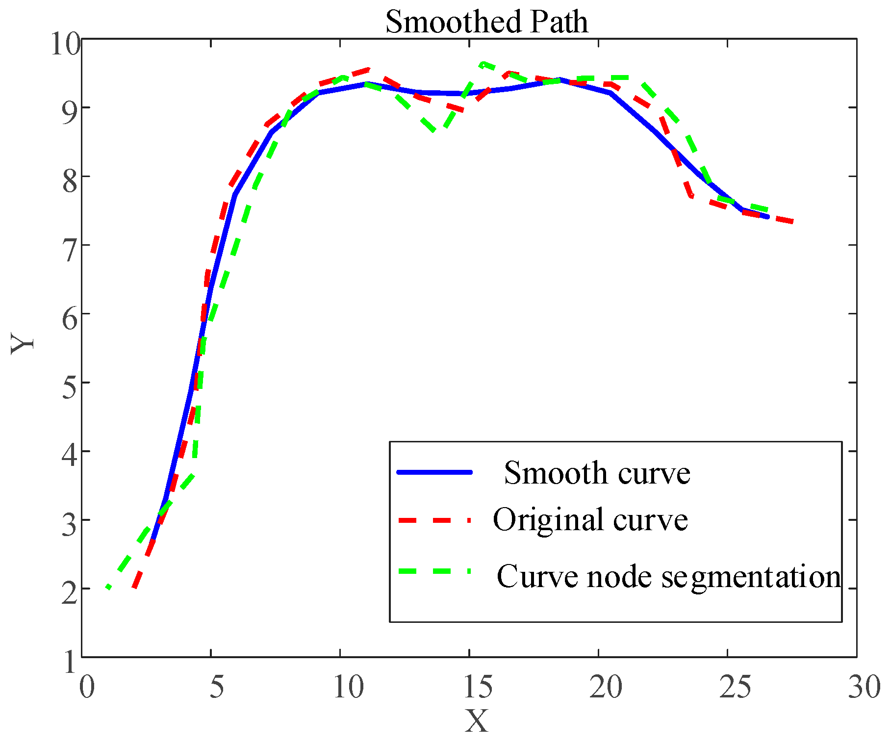
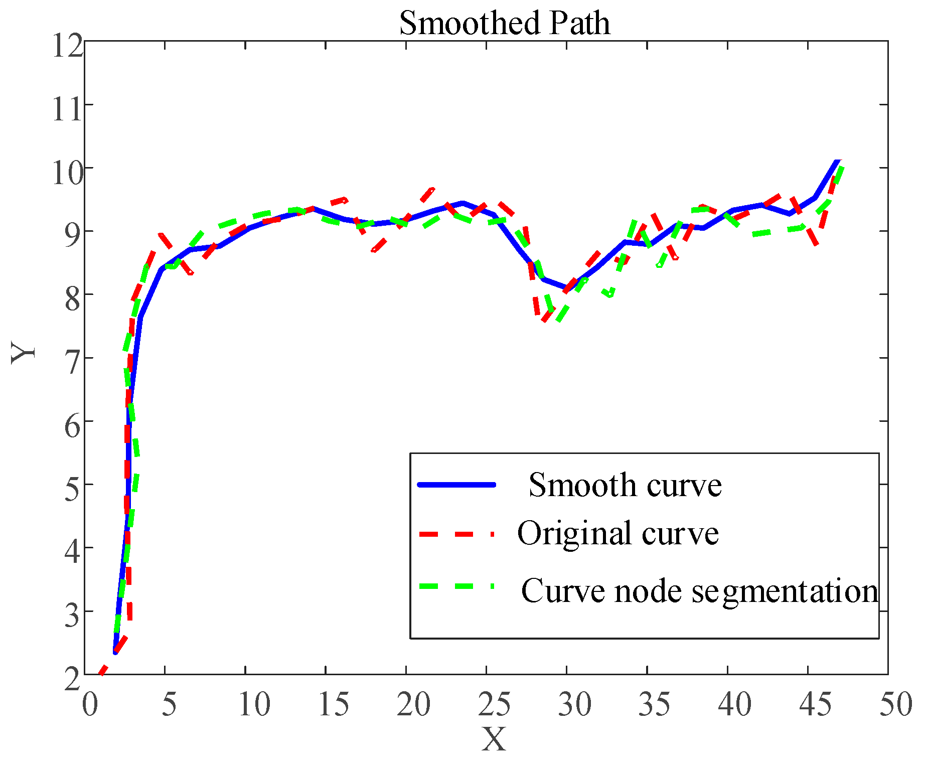
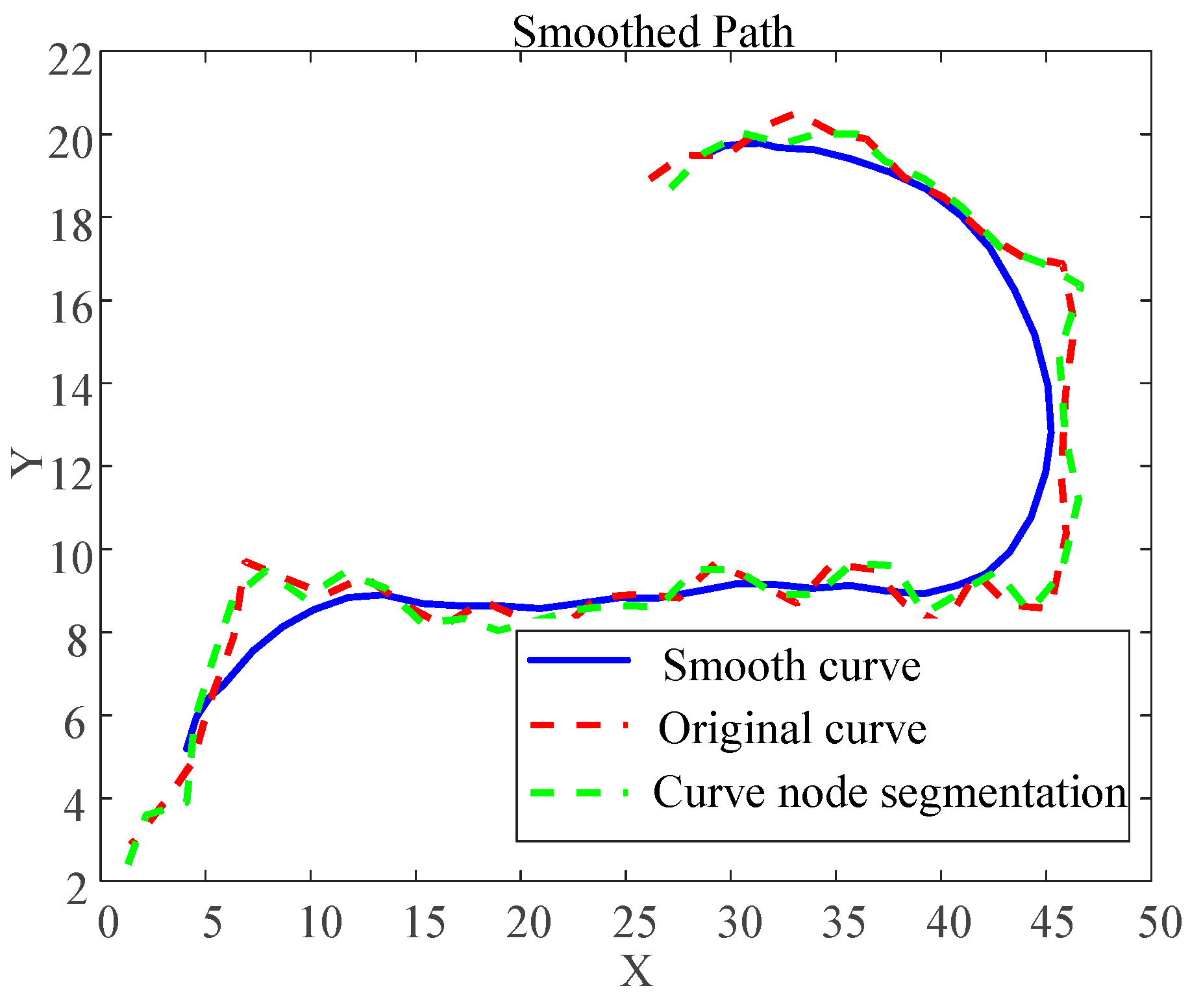
4.2. B-Spline Curve Path Optimization

After generating the path using the RRT algorithm, the points on the path are used as control points to construct a B-spline curve. To avoid obstacles, a nonlinear programming algorithm is employed to optimize the B-spline curve. Factors such as path smoothness, length, and distance from obstacles are treated as objective functions, transforming the path planning problem into an optimization problem. By solving this optimization problem, the optimal path is obtained.

Based on the above model, given the parameters, the path’s data is divided into curve segments and straight segments. The curve segments are smoothed, and the smoothed path data is then connected with the straight segments to plot the smoothed path. Next, the heading angle, velocity, acceleration, jerk, angular velocity, and angular acceleration are calculated based on the smoothed path data. The velocity, acceleration, and jerk are further smoothed, and finally, the graphs of these parameters over time are plotted.

Figure 11 shows the vehicle starting from the parking lot entrance, navigating through a curve, and stopping near the parking space on the upper side. The final parking position is the 10th space.

Figure 12 illustrates the smoothed trajectory for the 10th parking space. The vehicle gradually accelerates to approximately 7 km/h and then decelerates until it reaches the destination at around 17 s. At the stopping moment, the vehicle’s heading angle is −8.5°, positioning it relatively parallel to the driving path near the designated parking space.

Figure 13 depicts the vehicle starting from the parking lot entrance, navigating through two curves, and stopping near the parking space on the upper side. The final parking position is the 31st space.

Figure 14 presents the smoothed trajectory parameters for the 31st angled parking space. The vehicle’s motion characteristics, including velocity, acceleration, and jerk, are analyzed and visualized over time.

Figure 15 shows the vehicle starting from the parking lot entrance, navigating through two curves, and stopping near the parking space on the upper side. The final parking position is the 82nd space.

As seen in Figure 16, the vehicle gradually accelerates to approximately 7 km/h and then decelerates. At 30 s, the vehicle accelerates again, and around 34 s, it begins to decelerate until it reaches the destination at approximately 44 s. The heading angle shows an overall downward trend, indicating that the vehicle is making a right turn during its motion. At the stopping moment, the vehicle’s heading angle is −182.2°, positioning it relatively parallel to the driving path near the designated parking space. Graphs of angular velocity over time show large changes in angular velocity at the turns of the path and essentially zero angular velocity in the straight-line segments. Physically, the peak recorded at the limit of the maximum steering rate reflects the algorithm’s choice to concentrate heading adjustments in a single maneuver. This strategy minimizes intermediate heading changes and improves overall smoothness.

Based on the plotted graphs, the following conclusions can be drawn:

(1)

The smoothed path is significantly smoother than the original path, with more continuous curvature changes in the curve segments.

(2)

The time-varying graphs show that the velocity, angular velocity, acceleration, angular acceleration, and jerk exhibit smaller variations at the turning points of the path, while these parameters remain mostly constant in the straight segments.

4.3. Algorithm Validation

To validate the reliability of the algorithm, we conducted simulation experiments under three typical parking scenarios (vertical parking, diagonal parking, and parallel parking) to compare the PSBi-RRT algorithm, Bi-RRT algorithm, and RRT algorithm. Each scenario included all corresponding parking spaces, and the starting point configurations and obstacle layouts were similar across all cases. In total, there were 83 parking spaces, with each space tested 100 times, resulting in 8300 data points for each algorithm. The vehicle model adheres to typical kinematic constraints and employs a standard occupancy grid model for collision detection. In each set of experiments, both algorithms were run under identical conditions. We defined the following five key performance metrics for evaluation: path length, total steering angle change, planning time, number of expanded nodes, and success rate. These metrics are widely adopted in the evaluation of automated parking paths. All experiments recorded the aforementioned metrics for subsequent statistical analysis.

The definitions of each metric are as follows: The path length is the total distance traveled by the vehicle from the starting point to the endpoint, which is measured in meters; the total heading angle change refers to the cumulative directional change of the vehicle along the path, reflecting the frequency and amplitude of steering, which is measured in degrees; the planning time is the time required from algorithm startup to finding the final path, which is measured in seconds; the number of expanded nodes refers to the total number of nodes added to the tree structure during the search process, reflecting the algorithm’s exploration breadth and resource consumption in the state space; the success rate is the ratio of the number of successful paths found in physical verification to the total number of experiments. These metrics comprehensively evaluate the algorithm’s performance in terms of efficiency and robustness. Each location algorithm was iterated 100 times, and the average value was calculated. The specific experimental results are shown in

Table 2. Performance of the three algorithms in different parking spaces.

Parking Type	Algorithm	Path Length	Heading Change	Time	Node Count	Success Rate
Vertical	RRT	75.66	1076.27°	1.069	607.3	47.20%
Vertical	Bi-RRT	75.41	1046.75°	9.061	573.5	80.20%
Vertical	PSBi-RRT	74.74	974.18°	0.856	313.5	84.51%
Angled	RRT	46.39	511.26°	0.570	588	40.10%
Angled	Bi-RRT	47.11	523.62°	0.629	94.2	66.67%
Angled	PSBi-RRT	45.21	478.01°	0.261	64.5	90.66%
Parallel	RRT	25.39	305.89°	0.135	597	37.43%
Parallel	Bi-RRT	25.89	281.21°	2.513	84.4	90.95%
Parallel	PSBi-RRT	24.36	222.22°	0.046	56	92.57%

.

To further assess the statistical significance of the observed differences, we treated each parking spot’s 100 runs as a single unit by averaging, yielding 83 statistical units per algorithm. We then conducted one-way ANOVA on four continuous metrics—path length, total heading change, planning time, and node count—and a chi-square test on the success rate. The ANOVA results are as follows: The path length is F(2, 246) = 0.0024, p = 0.998 (>0.05), indicating no significant difference among RRT, Bi-RRT, and PSBi-RRT; the total heading change is F(2, 246) = 0.0794, p = 0.92 (>0.05), again showing no significant difference in cumulative steering; the planning time is F(2, 246) = 8.46, p = 0.018 (<0.05), where a post hoc Tukey HSD test confirms that PSBi-RRT is significantly faster than both Bi-RRT and RRT (p < 0.05); the node count is F(2, 246) = 8.47, p = 0.02 (<0.05), with post hoc comparisons likewise showing PSBi-RRT uses significantly fewer nodes than the two control algorithms (p < 0.05). These findings indicate that while all three methods yield comparable path quality (length and smoothness), PSBi-RRT offers a statistically significant advantage in computational efficiency (planning time) and search cost (node count), thereby underscoring the practical benefits of our proposed approach.

Specifically, vertical parking scenarios present the greatest challenge in path planning due to the need to perform a U-turn maneuver. In vertical parking environments, where space is limited, path planning algorithms face stringent requirements. Experimental data shows that PSBi-RRT performs best across five metrics: It generates the shortest path length and the smallest heading angle change; its planning time and number of nodes are significantly lower than those of RRT and Bi-RRT, and its success rate is the highest, exceeding that of the latter. Specifically, compared to the traditional Bi-RRT, PSBi-RRT reduces runtimes by 74.34%, reduces the number of nodes by 45.24%, and increases the success rate by 4.31%; the improvements are even more significant compared to unidirectional RRT. Due to the limited spatial constraints in vertical parking scenarios, traditional RRT/Bi-RRT algorithms often generate a large number of redundant nodes, leading to circuitous paths and significantly increased path costs. The bidirectional search and target-biased sampling strategy of PSBi-RRT effectively mitigates this issue, resulting in a substantial improvement in overall performance in this scenario.

Compared to vertical parking, diagonal parking offers more spacious areas with relatively simpler obstacle layouts. In this scenario, all metrics of the three algorithms improved, but PSBi-RRT remained the most optimal. The simulation results showed that PSBi-RRT generated the shortest path length, minimal heading changes, and lower planning time and node counts compared to Bi-RRT and RRT while also achieving the highest success rate. Due to the more open space, the search efficiency of traditional algorithms is generally higher, with Bi-RRT’s bidirectional growth significantly reducing pathfinding time. However, PSBi-RRT further optimizes the search process through target-biased sampling and node correction strategies. Target-biased sampling guides the process to approach the target area faster, reducing unnecessary random expansion; node correction maintains path smoothness and removes unnecessary turns. This enables PSBi-RRT to converge to high-quality paths more quickly in relatively spacious environments. Specifically, compared to traditional Bi-RRT, PSBi-RRT reduces the runtime by 58.50%, reduces the number of nodes by 31.52%, and improves the success rate by 23.99%; the performance improvement is even more significant compared to unidirectional RRT.

Compared with the other two scenarios, path planning for parallel parking spaces is the simplest, with the vehicle path mainly consisting of a straight line into the parking space. In this scenario, all three algorithms showed improvements in all metrics, but PSBi-RRT remained the best. Simulation results showed that PSBi-RRT still generated the shortest path length, the smallest heading change, and lower planning times and node counts than Bi-RRT and RRT, and it also had the highest success rate. Specifically, compared to the traditional Bi-RRT, PSBi-RRT reduces runtime by 98.16%, reduces the number of nodes by 33.64%, and increases the success rate by 1.62%; compared to the unidirectional RRT, the improvements are even more significant.

The PSBi-RRT algorithm demonstrates significant overall performance advantages across three distinct parking scenarios. Compared to the traditional RRT, PSBi-RRT achieves superior results across all evaluation metrics: shorter planned paths, smoother heading angle changes, an average reduction in planning time of 60.06%, a 76% reduction in the number of nodes, and a 47.67% increase in success rate. Compared to the Bi-RRT, PSBi-RRT achieves shorter planned paths, smoother heading angle changes, an average reduction in planning time of 78.33%, an average reduction in the number of nodes of 36.8%, and a 9.97% increase in success rate. The fundamental reason lies in the multi-faceted optimizations in the algorithm’s structure: The bidirectional random tree search strategy accelerates the connectivity of the path search, target-biased sampling makes the sampling process more directional, and node correction and path pruning further eliminate redundant paths. Therefore, in various space-constrained or obstacle-complex parking scenarios, PSBi-RRT provides more efficient and reliable path planning capabilities, fully validating its quantitative performance advantages and engineering application value.

5. Conclusions

In this study, the feasibility of the PSBi-RRT algorithm for autonomous parking applications was evaluated using MATLAB 2019b. Path planning was conducted in a specified parking lot, and the generated paths were optimized using B-spline curves, resulting in smooth and obstacle-free trajectories that enabled collision-free navigation to different parking spaces. Compared to traditional RRT, PSBi-RRT generates shorter planning paths, smoother heading angle changes, an average reduction in planning time of 60.06%, a 76% reduction in the number of nodes, and a 47.67% increase in success rate. Compared to Bi-RRT, PSBi-RRT generates shorter planning paths, smoother heading angle changes, an average reduction in planning time of 78.33%, an average reduction in the number of nodes of 36.8%, and a 9.97% increase in success rate.

Although PSBi-RRT performs well in two-dimensional parking scenarios, it still has several limitations. First, when the state space is expanded to include high-dimensional information such as vehicle speed and acceleration, the computational complexity of random sampling and bidirectional expansion will significantly increase, potentially leading to reduced real-time performance and lower success rates. Second, the current experiments were conducted on desktop-level hardware. If directly deployed to an in-vehicle embedded control unit, the limited computing power and memory may cause collision detection and sampling operations to become bottlenecks. Furthermore, when integrating the algorithm into the vehicle ECU, factors such as sensor data latency, real-time operating system interfaces, and coordination with the underlying controller must be considered, as these can impact the executability and stability of the planning results. To address these challenges, future work will focus on three areas of improvement: first, developing hybrid heuristic sampling strategies suitable for high-dimensional state spaces to mitigate the performance degradation caused by dimensionality growth; second, parallelizing the collision detection and sampling modules and optimizing data structures for common scenarios to reduce computational latency; third, conducting embedded prototype deployment and testing to evaluate the algorithm’s performance in resource-constrained and real-time communication environments and collaborating with the chassis control system for optimization to ensure the reliable implementation of the algorithm on actual intelligent vehicle platforms.

References

1. Selvaraj, S.; Thangarajan, R.; Rithik, J.R.A.; Pranesan, S.; Karthika, M. Intelligent parking assistance using deep reinforcement learning and YOLOv8 in simulated environments. In Proceedings of the 2025 International Conference on Multi-Agent Systems for Collaborative Intelligence (ICMSCI), Erode, India, 20–22 January 2025; IEEE: Piscataway, NJ, USA, 2025; pp. 1721–1728. [Google Scholar]
2. Huang, S.J.; Lin, G.Y. Parallel auto-parking of a model vehicle using a self-organizing fuzzy controller. Proc. Inst. Mech. Eng. Part D J. Automob. Eng. 2010, 224, 997–1012. [Google Scholar] [CrossRef]
3. Xu, X.; Xie, Y.; Li, R.; Zhao, Y.; Song, R.; Zhang, W. Hierarchical reinforcement learning for autonomous parking based on kinematic constraints. In Proceedings of the 2024 IEEE International Conference on Robotics and Biomimetics (ROBIO), Bangkok, Thailand, 10–14 December 2024; IEEE: Piscataway, NJ, USA, 2024. [Google Scholar]
4. Zhang, J.; Chen, H.; Song, S.; Hu, F. Reinforcement learning-based motion planning for automatic parking system. IEEE Access 2020, 8, 154485–154501. [Google Scholar] [CrossRef]
5. Gan, N.; Zhang, M.; Zhou, B.; Chai, T.; Wu, X.; Bian, Y. Spatio-temporal heuristic method: A trajectory planning for automatic parking considering obstacle behavior. J. Intell. Connect. Veh. 2022, 5, 177–187. [Google Scholar] [CrossRef]
6. LaValle, S. Rapidly-Exploring Random Trees: A New Tool for Path Planning; Iowa State University Research Report 9811. 1998, pp. 1–4. Available online: https://msl.cs.illinois.edu/~lavalle/papers/Lav98c.pdf (accessed on 1 July 2025).
7. Dong, Y.; Zhong, Y.; Hong, J. Knowledge-biased sampling-based path planning for automated vehicles parking. IEEE Access 2020, 8, 156818–156827. [Google Scholar] [CrossRef]
8. Wang, D.; Zheng, S.; Ren, Y.; Du, D. Path planning based on the improved RRT* algorithm for the mining truck. Comput. Mater. Contin. 2022, 71, 3571–3587. [Google Scholar] [CrossRef]
9. Wang, J.; Li, J.; Yang, J.; Meng, X.; Fu, T. Automatic parking trajectory planning based on random sampling and nonlinear optimization. J. Frankl. Inst. 2023, 360, 9579–9601. [Google Scholar] [CrossRef]
10. Jhang, J.H.; Lian, F.L. An autonomous parking system of optimally integrating bidirectional rapidly-exploring random trees and parking-oriented model predictive control. IEEE Access 2020, 8, 163502–163523. [Google Scholar] [CrossRef]
11. Jhang, J.H.; Lian, F.L.; Hao, Y.H. Human-like motion planning for autonomous parking based on revised bidirectional rapidly-exploring random tree* with Reeds-Shepp curve. Asian J. Control 2021, 23, 1146–1160. [Google Scholar] [CrossRef]
12. Meng, X.; Wang, N.; Liu, Q.; Sun, G. Aircraft parking trajectory planning in semistructured environment based on kinodynamic safety rrt. Math. Probl. Eng. 2021, 2021, 3872248. [Google Scholar] [CrossRef]
13. Kim, M.; Ahn, J.; Park, J. TargetTree-rrt*: Continuous-curvature path planning algorithm for autonomous parking in complex environments. IEEE Trans. Autom. Sci. Eng. 2022, 21, 606–617. [Google Scholar] [CrossRef]
14. Wang, W.; Li, J.; Bai, Z.; Wei, Z.; Peng, J. Toward optimization of AGV path planning: An RRT*-ACO algorithm. IEEE Access 2024, 12, 18387–18399. [Google Scholar] [CrossRef]
15. Ma, G.; Duan, Y.; Li, M.; Xie, Z.; Zhu, J. A probability smoothing bi-rrt path planning algorithm for indoor robot. FGCS 2023, 143, 349–360. [Google Scholar] [CrossRef]
16. Wang, J.; Li, T.; Li, B.; Meng, M.Q.-H. GMR-RRT*: Sampling-based path planning using gaussian mixture regression. IEEE Trans. Intell. Veh. 2022, 7, 690–700. [Google Scholar] [CrossRef]
17. Ganesan, S.; Ramalingam, B.; Mohan, R.E. A hybrid sampling-based rrt* path planning algorithm for autonomous mobile robot navigation. Expert Syst. Appl. 2024, 258, 125206. [Google Scholar] [CrossRef]
18. Caminiti, C.M.; Dimovski, A.; Edeme, D.; Carnovali, T.; Corigliano, S.; Gadelha, V.; Ragaini, E.; Merlo, M. The GISEle framework: Innovations in rural electrification planning. In Proceedings of the 2024 IEEE International Humanitarian Technologies Conference (IHTC), Bari, Italy, 27–30 November 2024; IEEE: Piscataway, NJ, USA, 2024; pp. 1–7. [Google Scholar]
19. Polack, P.; Altché, F.; d’Andréa-Novel, B.; de La Fortelle, A. The kinematic bicycle model: A consistent model for planning feasible trajectories for autonomous vehicles? In Proceedings of the 2017 IEEE Intelligent Vehicles Symposium (IV), Los Angeles, CA, USA, 11–14 June 2017; IEEE: Piscataway, NJ, USA, 2017; pp. 812–818. [Google Scholar]
20. Wu, B.; Qian, L.; Lu, M.; Qiu, D.; Liang, H. Optimal control problem of multi-vehicle cooperative autonomous parking trajectory planning in a connected vehicle environment. IET Intell. Transp. Syst. 2019, 13, 1677–1685. [Google Scholar] [CrossRef]
21. Yang, H.; Xu, X.; Hong, J. Automatic parking path planning of tracked vehicle based on improved A* and DWA algorithms. IEEE Trans. Transp. Electrif. 2022, 9, 283–292. [Google Scholar] [CrossRef]
22. Chen, L.; Shan, Y.; Tian, W.; Li, B.; Cao, D. A fast and efficient double-tree rrt* -like sampling-based planner applying on mobile robotic systems. IEEE/ASME Trans. Mechatron. 2018, 23, 2568–2578. [Google Scholar] [CrossRef]
23. Wang, B.; Ju, D.; Xu, F.; Feng, C.; Xun, G. CAF-RRT*: A 2D path planning algorithm based on circular arc fillet method. IEEE Access 2022, 10, 127168–127181. [Google Scholar] [CrossRef]
24. Han, Z.; Sun, H.; Huang, J.; Xu, J.; Tang, Y.; Liu, X. Path planning algorithms for smart parking: Review and prospects. World Electr. Veh. J. 2024, 15, 322. [Google Scholar] [CrossRef]
25. Cano, A.; Arévalo, P.; Benavides, D.; Jurado, F. Comparative analysis of HESS (battery/supercapacitor) for power smoothing of PV/HKT, simulation and experimental analysis. J. Power Sources 2022, 549, 232137. [Google Scholar] [CrossRef]
Figure 1. Schematic diagram of the outward expansion of the obstacle.
Wevj 16 00374 g001
Figure 2. Schematic diagram of the vehicle kinematics model.
Wevj 16 00374 g002
Figure 3. Equivalent rectangular schematic of the vehicle kinematics model.
Wevj 16 00374 g003
Figure 4. Flowchart of route planning.
Wevj 16 00374 g004
Figure 5. Schematic diagram of the Bi-RRT algorithm for node sampling.
Wevj 16 00374 g005
Figure 6. Parking lot layout.
Wevj 16 00374 g006
Figure 7. Layout of selected parking spaces for algorithm validation.
Wevj 16 00374 g007
Figure 8. Trajectory for the 10th vertical parking space. The red line shows the final planned route. The black lines show the additional paths that were explored. The blue area indicates the target area.
Wevj 16 00374 g008
Figure 9. Trajectory for the 31st angled parking space. The red line shows the final planned route. The black lines show the additional paths that were explored. The blue area indicates the target area.
Wevj 16 00374 g009
Figure 10. Trajectory for the 82nd parallel parking space. The red line shows the final planned route. The black lines show the additional paths that were explored. The blue area indicates the target area.
Wevj 16 00374 g010
Figure 11. Smoothed trajectory for 10th vertical parking space.
Wevj 16 00374 g011
Figure 12. Smoothed trajectory parameters for the 10th vertical parking space.
Wevj 16 00374 g012
Figure 13. Smoothed trajectory for the 31st angled parking space.
Wevj 16 00374 g013
Figure 14. Smoothed trajectory parameters for the 31st angled parking space.
Wevj 16 00374 g014
Figure 15. Smoothed trajectory for the 82nd parallel parking space.
Wevj 16 00374 g015
Figure 16. Trajectory parameters for the 82nd parallel parking space.
Wevj 16 00374 g016