
Comparative Study of Discretization Methods for Non-Ideal Proportional-Resonant Controllers in Voltage Regulation of Three-Phase Four-Wire Converters with Vehicle-to-Home Mode


Abstract
1. Introduction
2. Proportional-Resonant Controller
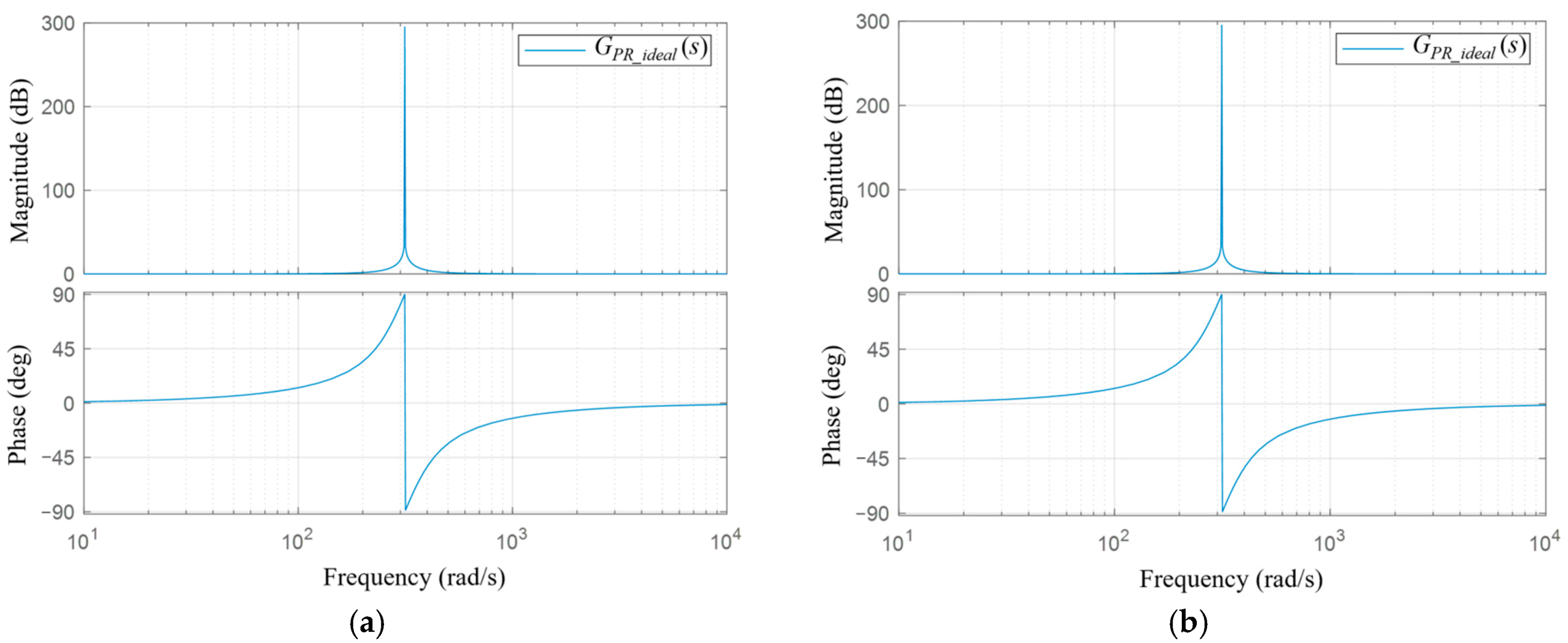
2.1. Ideal Proportional-Resonant Controller
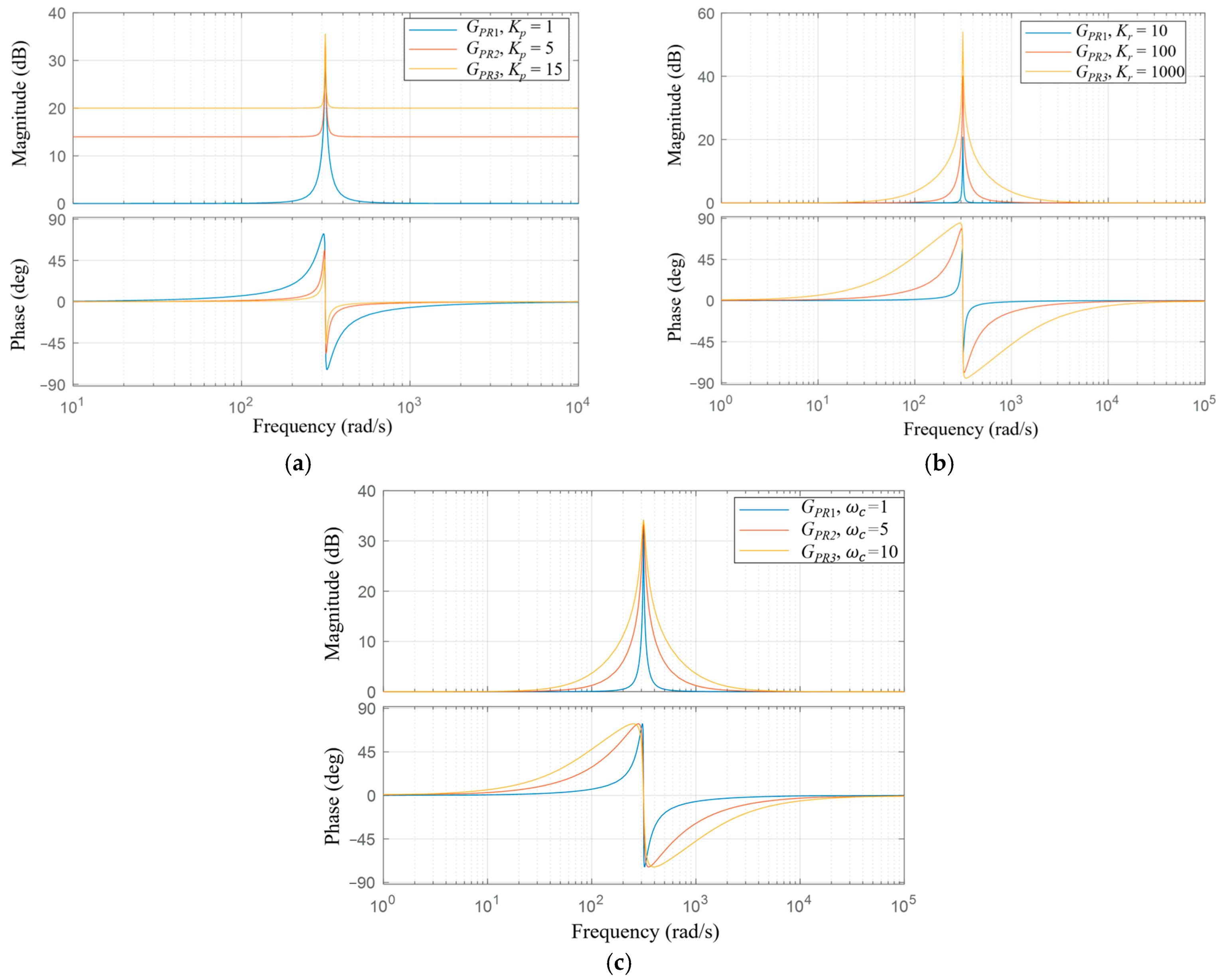
2.2. Non-Ideal Proportional-Resonant Controller
3. Discretization Implementations of Non-Ideal Proportional-Resonant Controllers
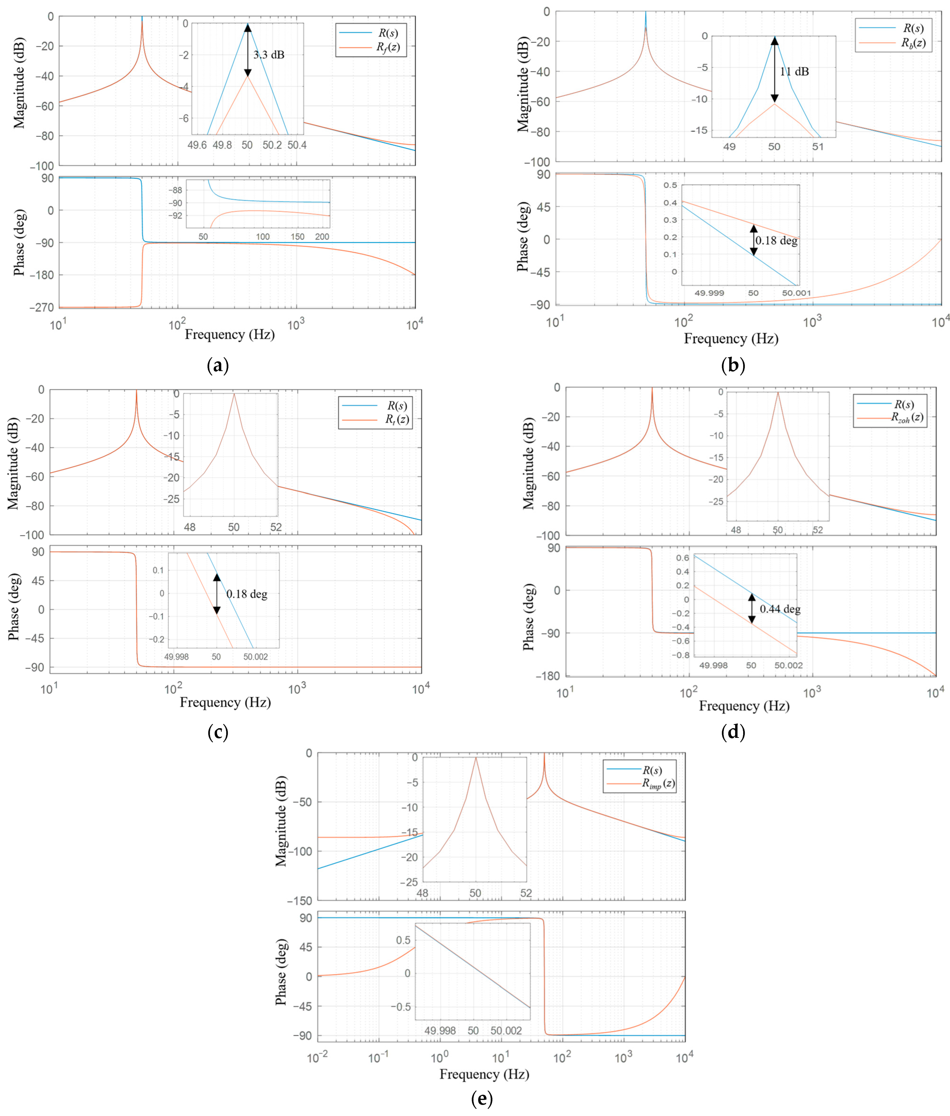
3.1. Discretization of Continuous-Time Complete Transfer Function
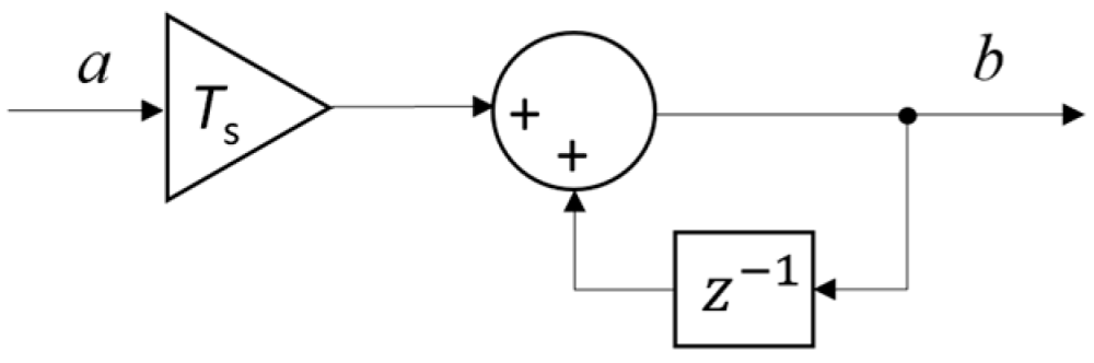
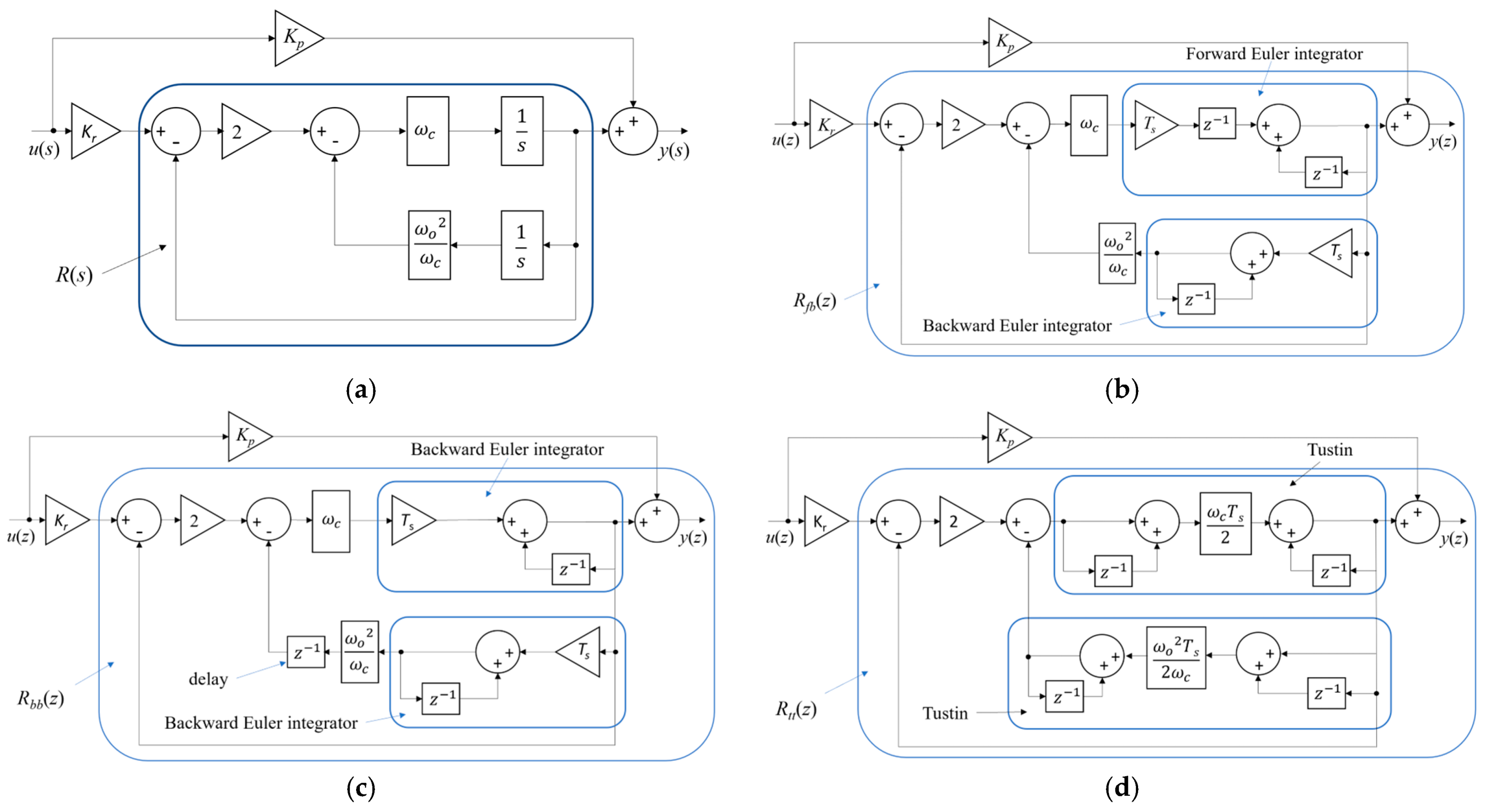
3.2. Discretization Using Discrete Integrators
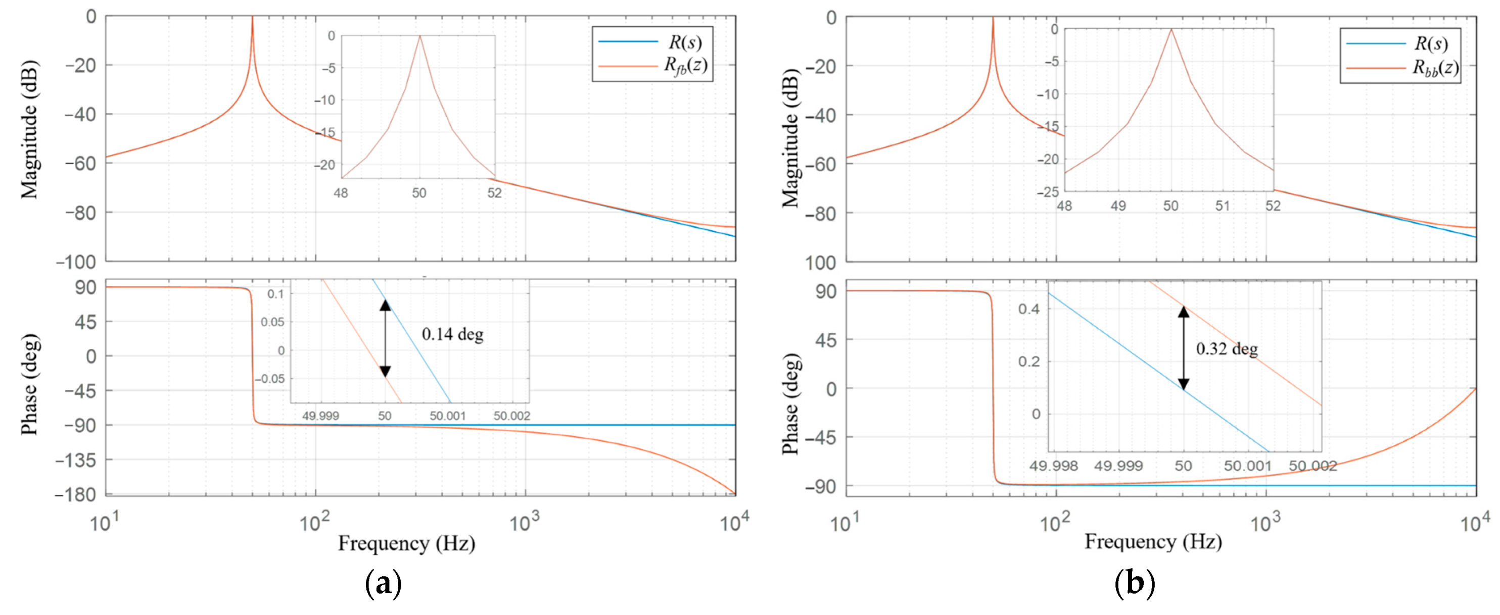
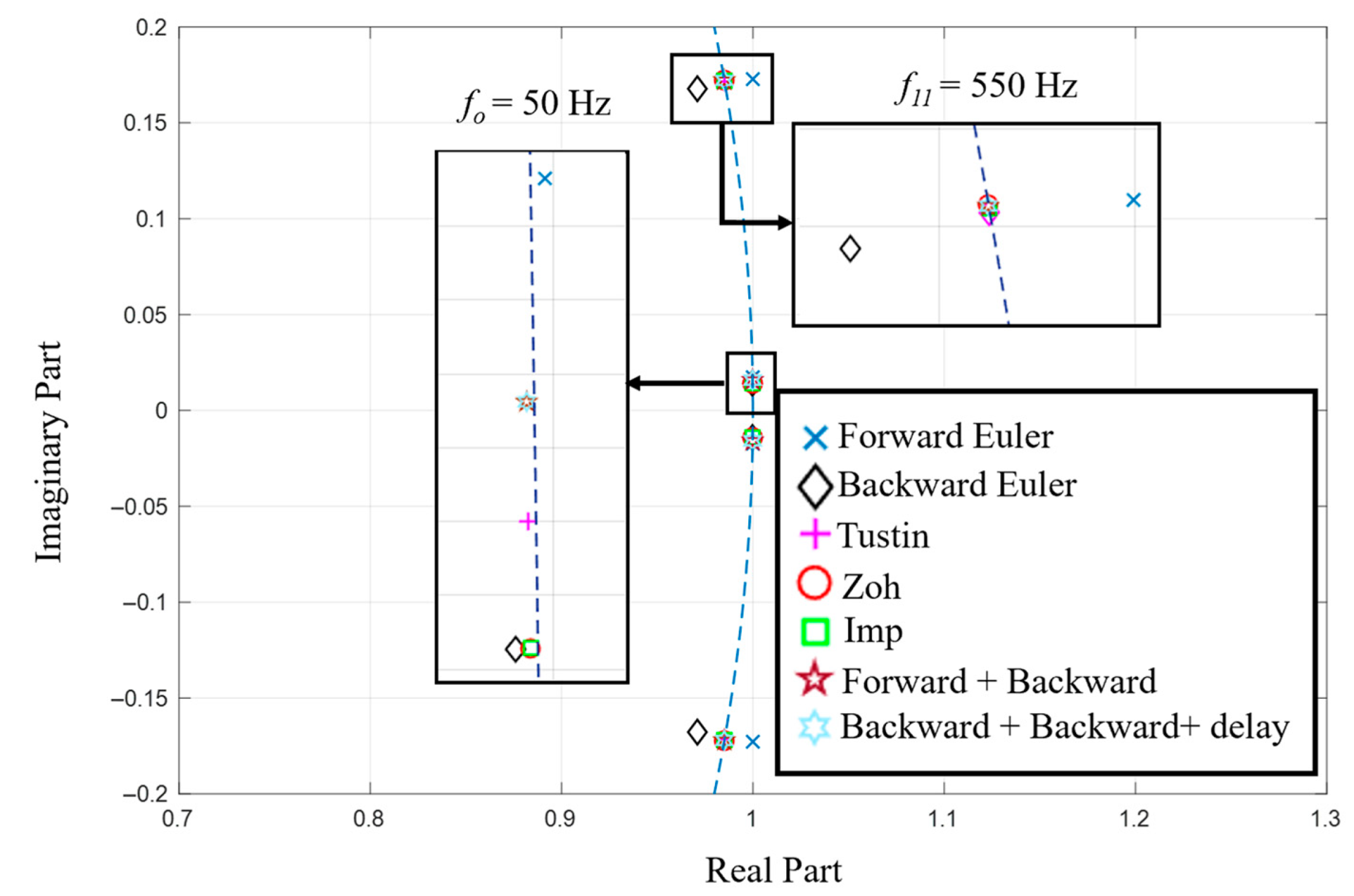
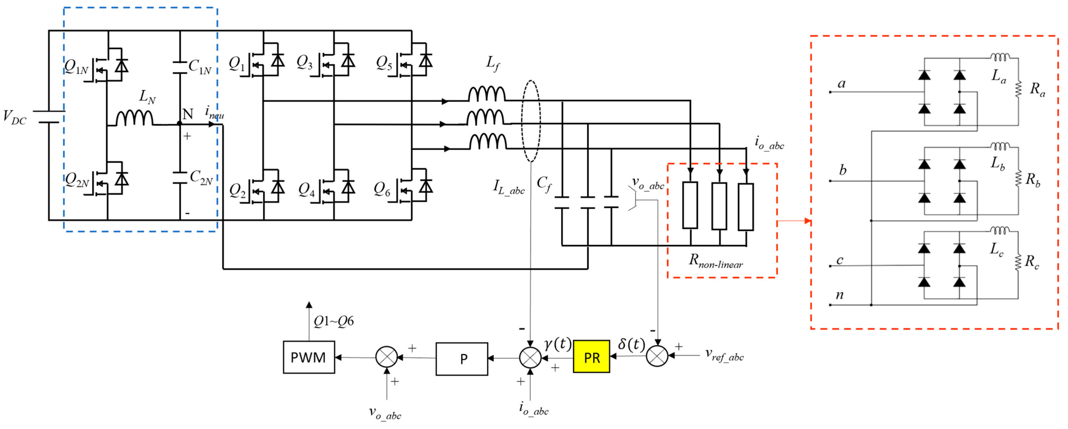
4. Simulation Results
5. Conclusions
Funding
Institutional Review Board Statement
Informed Consent Statement
Data Availability Statement
Conflicts of Interest
Abbreviations
| Abbreviations | |
| V2G | Vehicle to grid |
| V2L | Vehicle to load |
| V2H | Vehicle to home |
| 3P4W | Three-phase four-wire converter |
| THD | Total harmonic distortion |
| PI | Proportional integral |
| PR | Proportional resonant |
| PLL | Phase-locked loop |
| FLL | Frequency-locked loop |
| Symbols | |
| Transfer function of an ideal proportional-resonant controller | |
| Transfer function of a non-ideal proportional-resonant controller | |
| Kp | Proportional gain |
| Kr | Integral gain |
| Resonant angular frequency | |
| Resonance bandwidth | |
| R(s) | Resonant term of the non-ideal proportional-resonant controller in the s-domain |
| Rf(z) | Discretized resonant term of the non-ideal proportional-resonant controller using the Forward Euler method |
| Rb(z) | Discretized resonant term of the non-ideal proportional-resonant controller using the Backward Euler method |
| Rt(z) | Discretized resonant term of the non-ideal proportional-resonant controller using the Tustin method |
| Rzoh(z) | Discretized resonant term of the non-ideal proportional-resonant controller using the Zero-Order Hold method |
| Rimp(z) | Discretized resonant term of the non-ideal proportional-resonant controller using the Impulse-Invariant method |
| Rfb(z) | Discretized resonant term of the non-ideal proportional-resonant controller using the Forward Euler and Backward Euler method |
| Rbb(z) | Discretized resonant term of the non-ideal proportional-resonant controller using the Backward Euler and Backward Euler plus delay method |
| Rtt(z) | Discretized resonant term of the non-ideal proportional-resonant controller using the Tustin and Tustin method |
| fs | Sampling rate |
| Ts | Sampling period |
| fsw | Switching frequency |
| fbv | Bandwidth frequency |
| fo | Fundamental frequency. |
| Kpu | Proportional gain of the non-ideal PR controller |
| Kru | Integral gain of the non-ideal PR controller |
| Kpi | Proportional gain of the P controller |
| Ra | Phase-A load resistance |
| La | Phase-A load inductance |
| Rb | Phase-B load resistance |
| Lb | Phase-B load inductance |
| Rc | Phase-C load resistance |
| Lc | Phase-C load inductance |
| Lf | Inductor of LC filter |
| Cf | Capacitor of LC filter |
| LN | Neutral inductor |
| C1N | Upper split-capacitor |
| C2N | Lower split-capacitor |
| VDC | DC-link voltage |
| The input signal of the non-ideal PR controller | |
| The output signal of the non-ideal PR controller | |
Appendix A
Appendix A.1. Discretization of Continuous-Time Complete Transfer Function R(s)
Appendix A.1.1. Forward Euler Method
Appendix A.1.2. Backward Euler Method
Appendix A.1.3. Tustin Method
Appendix A.1.4. Zero-Order Hold Method
Appendix A.1.5. Impulse-Invariant Method
Appendix A.2. Discretization of Single Integrator Within Block Diagram of Non-Ideal PR Controllers in Figure 4a
Appendix A.2.1. Forward Euler Method

Appendix A.2.2. Backward Euler Method
Appendix A.2.3. Tustin Method

Appendix B. Addressing the Algebraic Loop Issue Encountered with the Tustin and Tustin Method in Figure 4d

References
- Yang, Y.; Benomar, Y.; Baghdadi, M.E.; Hegazy, O.; Mierlo, J.V. Design, Modeling and Control of a Bidirectional Wireless Power Transfer for Light-Duty Vehicles: G2V and V2G Systems. In Proceedings of the 2017 19th European Conference on Power Electronics and Applications (EPE’17 ECCE Europe), Warsaw, Poland, 11–14 September 2017; pp. P.1–P.12. [Google Scholar]
- Rosas, D.S.; Andrade, J.; Frey, D.; Ferrieux, J.P. Single Stage Isolated Bidirectional DC/AC Three-Phase Converter with a Series-Resonant Circuit for V2G. In Proceedings of the 2017 IEEE Vehicle Power and Propulsion Conference (VPPC), Belfort, France, 14–17 December 2017; pp. 1–5. [Google Scholar]
- Wang, X.; Liu, Y.; Qian, W.; Wang, B.; Lu, X.; Zou, K.; Santini, N.S.; Karki, U.; Peng, F.Z.; Chen, C. A 25kW SiC Universal Power Converter Building Block for G2V, V2G, and V2L Applications. In Proceedings of the 2018 IEEE International Power Electronics and Application Conference and Exposition (PEAC), Shenzhen, China, 4–7 November 2018; pp. 1–6. [Google Scholar]
- Wang, X.; Liu, Y.; Qian, W.; Janabi, A.; Wang, B.; Lu, X.; Zou, K.; Chen, C.; Peng, F.Z. Design, and Control of a SiC Isolated Bidirectional Power Converter for V2L Applications to both DC and AC Load. In Proceedings of the 2019 IEEE 7th Workshop on Wide Bandgap Power Devices and Applications (WiPDA), Raleigh, NC, USA, 29–31 October 2019; pp. 143–150. [Google Scholar]
- Wang, H.; Jia, X.; Li, J.; Guo, X.; Wang, B.; Wang, X. New single-stage EV charger for V2H applications. In Proceedings of the 2016 IEEE 8th International Power Electronics and Motion Control Conference (IPEMC-ECCE Asia), Hefei, China, 22–26 May 2016; pp. 2699–2702. [Google Scholar]
- Fu, Y.; Huang, Y.; Bai, H.; Lu, X.; Zou, K.; Chen, C. A High-efficiency SiC Three-Phase Four-Wire inverter with Virtual Resistor Control Strategy Running at V2H mode. In Proceedings of the 2018 IEEE 6th Workshop on Wide Bandgap Power Devices and Applications (WiPDA), Atlanta, GA, USA, 31 October–2 November 2018; pp. 174–179. [Google Scholar]
- Almughram, O.; Slama, S.B.; Zafar, B. Model for Managing the Integration of a Vehicle-to-Home Unit into an Intelligent Home Energy Management System. Sensors 2022, 22, 8142. [Google Scholar] [CrossRef] [PubMed]
- Pai, L.; Senjyu, T.; Elkholy, M.H. Integrated Home Energy Management with Hybrid Backup Storage and Storage and Vehicle-to-Home Systems for Enhanced Resilience, Efficiency, and Energy Independence in Green Buildings. Appl. Sci. 2024, 14, 7747. [Google Scholar] [CrossRef]
- Liu, S.; Vlachokostas, A.; Kontou, E. Leveraging electric vehicles as a resiliency solution for residential backup power during outages. Energy 2025, 318, 134613. [Google Scholar] [CrossRef]
- Fu, Y.; Huang, Y.; Bai, H.; Lu, X.; Zou, K.; Chen, C. Imbalanced Load Regulation Based on Virtual Resistance of A Three-Phase Four-Wire Inverter for EV Vehicle-to-Home Applications. IEEE Trans. Transp. Electrif. 2019, 5, 162–173. [Google Scholar] [CrossRef]
- Jeong, S.Y.; Nguyen, T.H.; Lee, D.C.; Kim, J.M. Nonlinear control of three-phase four-wire dynamic voltage restorers for distribution system. In Proceedings of the 2014 International Power Electronics Conference (IPEC-Hiroshima 2014–ECCE ASIA), Hiroshima, Japan, 18–21 May 2014; pp. 2406–2412. [Google Scholar]
- Lin, Z.; Ruan, X.; Jia, L.; Zhao, W.; Liu, H.; Rao, P. Optimized Design of the Neutral Inductor and Filter Inductors in Three-Phase Four-Wire Inverter with Split DC-Link Capacitors. IEEE Trans. Power Electron. 2019, 34, 247–262. [Google Scholar] [CrossRef]
- Sun, S.; Huang, Q.; Luo, B.; Lu, J.; Luo, J.; Ma, Z.; Zhu, G. An Energy-Feed Type Split-Capacitor Three-Phase Four-Wire Power Electronic Load Compatible with Various Load Demands. Energies 2024, 17, 119. [Google Scholar] [CrossRef]
- Jiang, Z.; Yu, X. Active power—Voltage control scheme for islanding operation of inverter-interfaced microgrids. In Proceedings of the 2009 IEEE Power & Energy Society General Meeting, Calgary, AB, Canada, 26–30 July 2009; pp. 1–7. [Google Scholar]
- Nazifi, H.; Radan, A. Current control assisted and non-ideal Proportional-Resonant voltage controller for four-leg three-phase inverters with time-variant loads. In Proceedings of the 4th Annual International Power Electronics, Drive Systems and Technologies Conference, Tehran, Iran, 13–14 February 2013; pp. 355–360. [Google Scholar]
- Zhang, N.; Tang, H.; Yao, C. A Systematic Method for Designing a PR Controller and Active Damping of the LCL Filter for Single-Phase Grid-Connected PV Inverters. Energies 2014, 7, 3934–3954. [Google Scholar] [CrossRef]
- Zhou, P.; He, Y.; Sun, D. Improved direct power control of a DFIG- based wind turbine during network unbalance. IEEE Trans. Power Electron. 2009, 24, 2465–2474. [Google Scholar] [CrossRef]
- Teodorescu, R.; Blaabjerg, F.; Borup, U.; Liserre, M. A new control structure for grid-connected LCL PV inverters with zero steady-state error and selective harmonic compensation. IEEE Appl. Power Electron. 2004, 1, 580–586. [Google Scholar]
- Hu, J.; Li, D.; Lin, Z. Reduced Design of PR Controller in Selected Harmonic Elimination APF Based on Magnetic Flux Compensation. In Proceedings of the 2018 21st International Conference on Electrical Machines and Systems (ICEMS), Jeju, Republic of Korea, 7–10 October 2018; pp. 2090–2094. [Google Scholar]
- Hu, P.; He, Z.; Li, S.; Guerrero, J.M. Non-Ideal Proportional Resonant Control for Modular Multilevel Converters under SubModule Fault Conditions. IEEE Trans. Energy Convers. 2019, 34, 1741–1750. [Google Scholar] [CrossRef]
- Althobaiti, A.; Armstrong, M.; Elgendy, M.A. Current control of three-phase grid-connected PV inverters using adaptive PR controller. In Proceedings of the 2016 7th International Renewable Energy Congress (IREC), Hammamet, Tunisia, 22–24 March 2016; pp. 1–6. [Google Scholar]
- Seifi, K.; Moallem, M. An Adaptive PR Controller for Synchronizing Grid-Connected Inverters. IEEE Trans. Ind. Electron. 2019, 66, 2034–2043. [Google Scholar] [CrossRef]
- Mukherjee, S.; Shit, S.; Chakraborty, R.; Chatterjee, D. Design and analysis of Fuzzy tuned Proportional Resonant controller for Shunt Active Power filter using Neutral Point Clamped Multi-level Inverter. In Proceedings of the Michael Faraday IET International Summit, Kolkata, India, 12–13 September 2015; pp. 410–416. [Google Scholar]
- Yepes, A.G.; Freijedo, F.D.; Gandoy, J.D.; López, O.; Malvar, J.; Comesana, P.F. Effects of Discretization Methods on the Performance of Resonant Controllers. IEEE Trans. Power Electron. 2010, 25, 1692–1712. [Google Scholar] [CrossRef]
- Faria, J.; Fermeiro, J.; Pombo, J.; Calado, M.; Mariano, S. Proportional Resonant Current Control and Output-Filter Design Optimization for Grid-Tied Inverters Using Grey Wolf Optimizer. Energies 2020, 13, 1923. [Google Scholar] [CrossRef]
- Rodriguez, F.J.; Bueno, E.; Aredes, M.; Rolim, L.G.B.; Neves, F.A.S.; Cavalcanti, M.C. Discrete-time implementation of second order generalized integrators for grid converters. In Proceedings of the 2008 34th Annual Conference of IEEE Industrial Electronics, Orlando, FL, USA, 10–13 November 2008; pp. 176–181. [Google Scholar]
- Hintz, A.; Prasanna, R.; Rajashekara, K. Comparative study of three-phase grid connected inverter sharing unbalanced three-phase and/or single-phase systems. In Proceedings of the 2015 IEEE Energy Conversion Congress and Exposition (ECCE), Montreal, QC, Canada, 20–24 September 2015; pp. 6491–6496. [Google Scholar]
- Yang, P.; Ming, W.; Liang, J.; Wu, J. A Four-leg Buck Inverter for Three-phase Four-wire Systems with the Function of Reducing DC-bus Ripples. In Proceedings of the IECON 2019—45th Annual Conference of the IEEE Industrial Electronics Society, Lisbon, Portugal, 14–17 October 2019; pp. 1508–1513. [Google Scholar]
- Garganeev, A.G.; Aboelsaud, R.; Ibrahim, A. Voltage Control of Autonomous Three-Phase Four-Leg VSI Based on Scalar PR Controllers. In Proceedings of the 20th International Conference of Young Specialists on Micro/Nanotechnologies and Electron Devices (EDM), Lisbon, Portugal, 29 June–3 July 2019. [Google Scholar]


| Discretization Method | Equivalence | Notation |
|---|---|---|
| Forward Euler | Rf(z) | |
| Backward Euler | Rb(z) | |
| Tustin | Rt(z) | |
| Zero-Order Hold | Rzoh(z) | |
| Impulse Invariance | Rimp(z) |
| Discretization Method | Discretized R(s) |
|---|---|
| Forward Euler | |
| Backward Euler | |
| Tustin | |
| Zero-Order Hold | |
| Impulse Invariance |
| Parameters | Value | Parameters | Value |
|---|---|---|---|
| Kpu | 0.37 | 1 rad/s | |
| Kru | 150 | Kpi | 78 |
| rad/s |
| Parameters | Values |
|---|---|
| Phase-A load | Ra = 20 , La = 20 mH |
| Phase-B load | Rb = 20 , Lb = 20 mH |
| Phase-C load | Rc = 20 , Lc = 20 mH |
| Inductor of LC filter | Lf = 0.4 mH |
| Capacitor of LC filter | Cf = 20 |
| Split-capacitor of ICNM | C1N= C2N = 1000 |
| Neutral inductor of ICNM | LN = 2.8 mH |
| DC voltage | VDC = 650 V |
| Switching frequency | fsw = 20 kHz |
| Method | Voltage THD (%) | Current THD (%) |
|---|---|---|
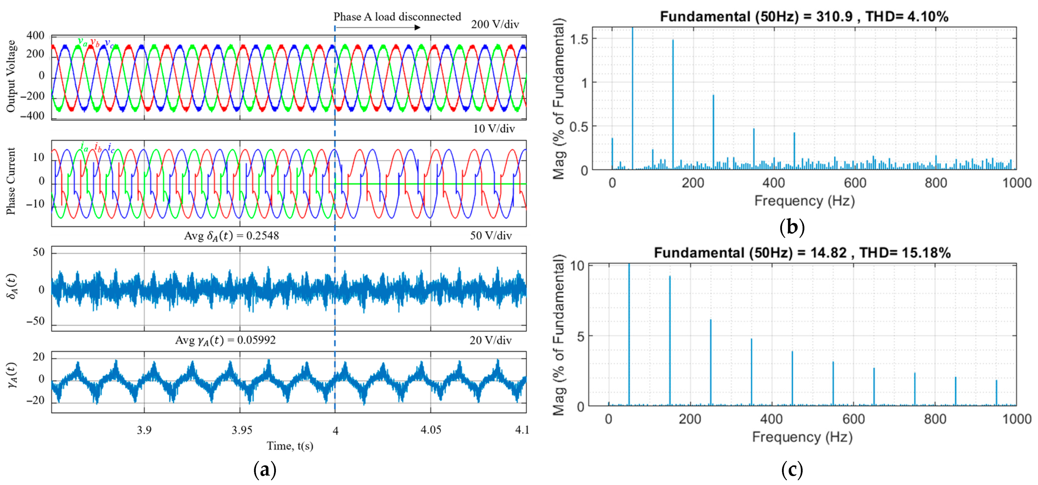
| Tustin | 4.10 | 15.18 |
| Zero-Order Hold | 4.02 | 15.26 |
| Impulse Invariance | 4.07 | 15.36 |
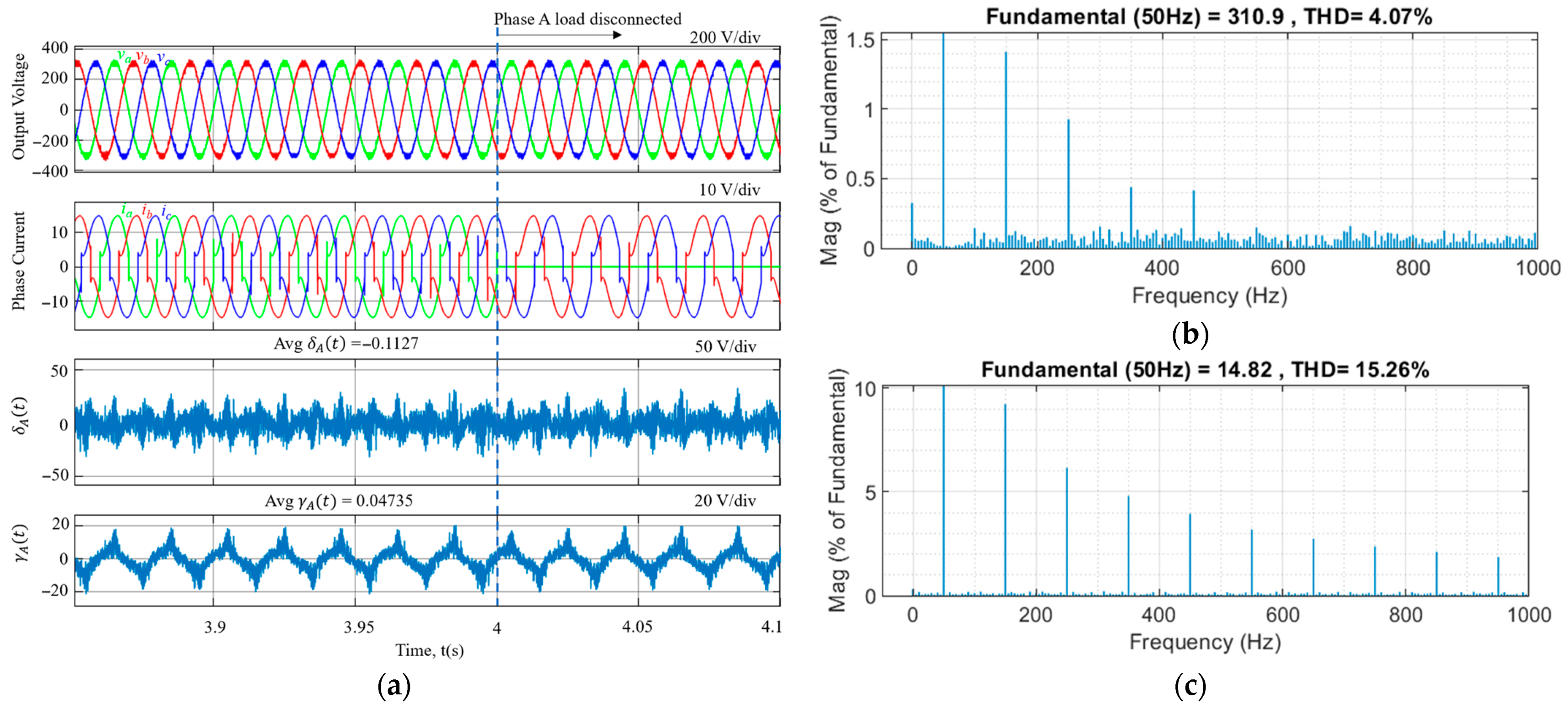
| Forward Euler and Backward Euler | 4.06 | 15.18 |
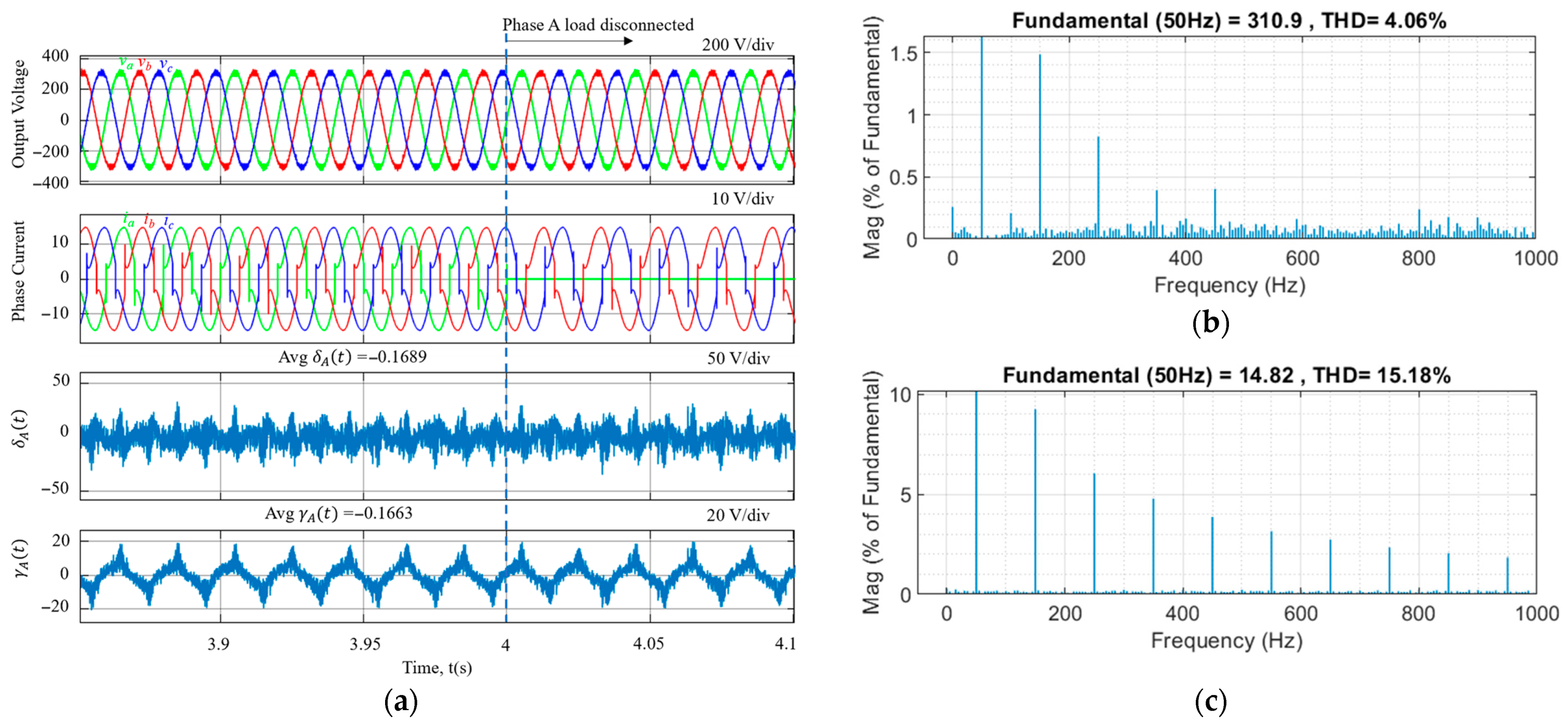
| Backward Euler and Backward Euler plus delay | 4.01 | 15.27 |
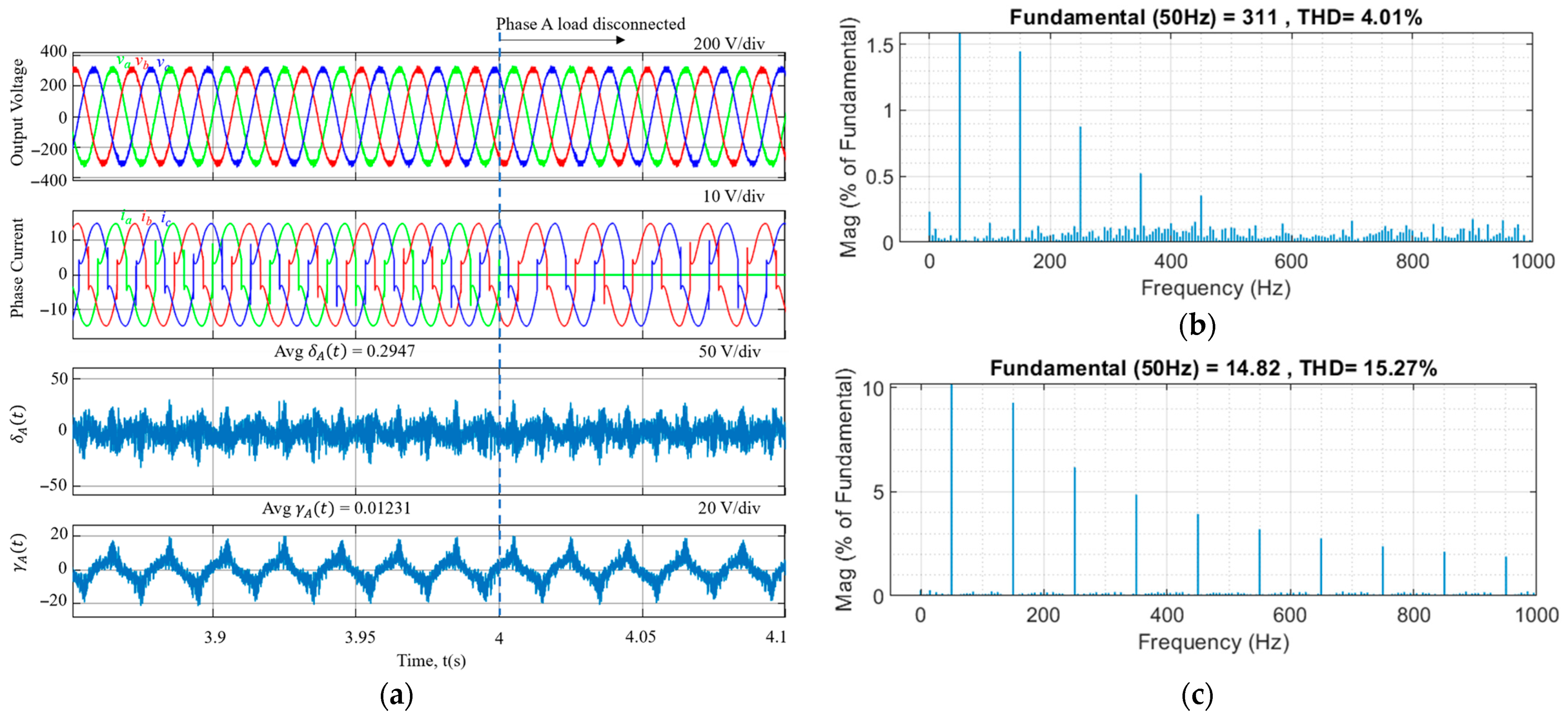
| Tustin and Tustin | 4.07 | 15.22 |
Disclaimer/Publisher’s Note: The statements, opinions and data contained in all publications are solely those of the individual author(s) and contributor(s) and not of MDPI and/or the editor(s). MDPI and/or the editor(s) disclaim responsibility for any injury to people or property resulting from any ideas, methods, instructions or products referred to in the content. |
© 2025 by the author. Published by MDPI on behalf of the World Electric Vehicle Association. Licensee MDPI, Basel, Switzerland. This article is an open access article distributed under the terms and conditions of the Creative Commons Attribution (CC BY) license (https://creativecommons.org/licenses/by/4.0/).
Share and Cite
Nguyen, A.T. Comparative Study of Discretization Methods for Non-Ideal Proportional-Resonant Controllers in Voltage Regulation of Three-Phase Four-Wire Converters with Vehicle-to-Home Mode. World Electr. Veh. J. 2025, 16, 335. https://doi.org/10.3390/wevj16060335
Nguyen AT. Comparative Study of Discretization Methods for Non-Ideal Proportional-Resonant Controllers in Voltage Regulation of Three-Phase Four-Wire Converters with Vehicle-to-Home Mode. World Electric Vehicle Journal. 2025; 16(6):335. https://doi.org/10.3390/wevj16060335
Chicago/Turabian StyleNguyen, Anh Tan. 2025. "Comparative Study of Discretization Methods for Non-Ideal Proportional-Resonant Controllers in Voltage Regulation of Three-Phase Four-Wire Converters with Vehicle-to-Home Mode" World Electric Vehicle Journal 16, no. 6: 335. https://doi.org/10.3390/wevj16060335
APA StyleNguyen, A. T. (2025). Comparative Study of Discretization Methods for Non-Ideal Proportional-Resonant Controllers in Voltage Regulation of Three-Phase Four-Wire Converters with Vehicle-to-Home Mode. World Electric Vehicle Journal, 16(6), 335. https://doi.org/10.3390/wevj16060335