Research on the Evaluation of Urban Green Transportation Development Level in Guangzhou Under the Promotion of New Energy Vehicles

Abstract

Assessing the urban green transportation development level (UGTDL) is of great significance for addressing traffic issues in megacities and promoting urban sustainable development. An evaluation framework for the UGTDL is proposed based on Multi-Criteria Decision Analysis (MCDA) methods. Firstly, from both macro and micro perspectives, a comprehensive evaluation indicator system is constructed, covering multiple dimensions such as traffic spatial organization efficiency, green travel, new energy vehicle development, traffic safety, and the traffic environment. Secondly, to address the uncertainties and fuzziness in the evaluation process, the Probability Language Term Set (PLTS) is introduced to represent expert evaluation information, thereby reducing the information loss. Thirdly, the improved Step-wise Weight Assessment Ratio Analysis (SWARA) method is employed to calculate the weights of the indicators, improving the computational efficiency. Finally, the extended Combined Compromise Solution (CoCoSo) method is used to calculate the UGTDL, avoiding the compensatory issues in the traditional decision-making methods. The proposed approach is applied to assess the UGTDL in Guangzhou from 2020 to 2023. The results show that the UGTDL scores for Guangzhou from 2020 to 2023 are 1.6367, 2.2325, 2.1141, and 1.8575, respectively. Sensitivity analysis verifies the effectiveness and stability of the approach. Further obstacle analysis shows that the promotion of new energy vehicles (NEVs) has led to a marginal decrease in the utility of Guangzhou’s UGTDL. In the future, Guangzhou should take further measures to improve the traffic space organization efficiency and traffic safety.

1. Introduction

With the increasingly severe global climate change and energy crisis, new energy vehicles (NEVs), as important green transportation tools, have become key measures in the green transformation of urban transport. In November 2020, the Chinese government released the “New Energy Vehicle Industry Development Plan (2021–2035)” with the target of achieving a 40% market penetration rate for (NEVs) by 2030 to promote energy transition and sustainable development in the transportation sector [1]. Driven by this policy, the promotion of NEVs in major cities across China has made significant progress, becoming an important part of the green transportation system. However, as NEVs become more widespread, the sole focus on “NEV promotion” will no longer be the key limiting factor for urban green transportation development. Other bottlenecks, such as transportation infrastructure construction, the optimization of public transport systems, and transportation behaviors, may become significant obstacles to further urban green transportation development. Therefore, how to comprehensively evaluate and identify the current status and potential constraints of urban green transportation development under the promotion of NEVs will provide guidance for the improvement and implementation of future urban green transportation policies.

The evaluation of the urban green transportation development level (UGTDL) has become a popular research topic. Several studies have explored this topic [2,3,4,5,6,7,8,9] (as shown in

Table 1. Major studies on urban green transportation development evaluation.

Authors	Research Methods	Research Areas
Wang et al. [2]	Analytic Hierarchy Process (AHP), Entropy Method	Chongqing (China)
Wang et al. [3]	Entropy Method, Grey Relational Analysis Method (GRA)	Lanzhou (China)
Pan et al. [4]	Entropy Method, GRA Method, Technique for Order Preference by Similarity to Ideal Solution (TOPSIS)	Wuhan (China)
Deng et al. [5]	Ordinal Relationship Analysis (G1) Method, Entropy Method, Addition Integration Method	Harbin (China)
Zhang et al. [6]	DEMATEL, Entropy Method, Fuzzy AHP	30 Cities (China)
Shen et al. [7]	Entropy Method, TOPSIS	Zhoushan (China)
Yu et al. [8]	Entropy Method, TOPSIS, Obstacle Degree Model	National Central Cities (China)
Kraus et al. [9]	Integrative Structural Modeling with Polarity (ISM-P), Preference Preference Ranking Organization Method for Enrichment Evaluations (PROMETHEE) method	Ruhr region (Germany)

). According to the findings of reference [2], Yuzhong is identified as the district with the highest level of green transportation development in Chongqing, while Jiulongpo is ranked the lowest. The assessment results in reference [3] reveal that the green transportation development level in Lanzhou experienced a rise, followed by a decline and then another rise from 2011 to 2017, indicating an overall upward trend. Reference [4] indicates that from 2015 to 2019, Wuhan’s green transportation development level exhibited a slight fluctuation with an overall increasing trend, achieving a comprehensive growth of 61.3%. The main limiting factors influencing this development shifted from the proportion of NEVs, public transportation share, and transportation noise levels to indicators such as per capita road area and pedestrian pathway area. Reference [5] evaluates Harbin’s green transportation in 2021 as being at a “good” level, though its public transport service still requires further improvement. Reference [6], which analyzed 30 provincial capital and central cities in China, reports an average composite score of 2.871 for green transportation development, suggesting a moderate level overall. Between 2011 and 2020, the cities’ scores showed a trend of “initial decline—fluctuating rise—subsequent decline”. Reference [7] finds that Zhoushan’s green transportation development in 2017 outperformed that of 2018 and was also superior to that in 2016. The study in reference [8] identifies total passenger transport volume, taxi ownership, NEV production, transport expenditure, and freight volume as the main obstacles to the UGTDL in China’s national central cities. Finally, reference [9] highlights that public transportation services are the primary driver of sustainable urban green transportation development.

According to Table 1, the existing studies mostly focus on general cities or specific types of cities, such as mountainous cities or valley-type cities, while there is relatively little research on megacities with significant transportation environmental problems. Furthermore, most of the existing studies have employed Multi-Criteria Decision Analysis (MCDA) methods such as AHP, the entropy method, TOPSIS, and PROMETHEE to evaluate the UGTDL, indicating that UGTDL evaluation is a typical MCDA problem. However, with the continuous development of MCDA methods, novel and advanced MCDA models have been widely developed and applied in supply chain management [10], financial engineering [11,12], the hydrological environment [13], aviation transportation [14], biomedical engineering [15], and energy management [16]. In comparison, the development of urban green transportation evaluation models has been relatively slow. There is a clear need for the development of new MCDA models that provide better evaluation results in urban green transportation evaluation. Typically, the construction of an MCDA model involves three issues: (1) the representation of evaluation information, which refers to the appropriate quantification of indicators for the evaluation object; (2) the determination of the weights of indicators; and (3) the ranking of the evaluation objects.

Regarding the representation of evaluation information, due to the complexity, fuzziness, and multi-level nature of the real-world decision-making environment, decision information is often difficult to express using precise real numbers [17]. Therefore, Zadeh [18] proposed the concept of Linguistic Term Sets (LTSs) to represent fuzzy decision information, expanding the application of decision theory [19]. Subsequently, scholars proposed various new types of LTS, such as 2-tuple LTS [20], Pythagorean fuzzy linguistic sets (PFLS) [21], intuitionistic fuzzy linguistic sets (IFLSs) [22], and hesitant fuzzy linguistic term sets (HFLTS) [23], to deal with the uncertainty and hesitation in decision making. However, these LTSs do not consider the frequency or importance of linguistic term elements (LTEs) in decision information. Therefore, Pang et al. [24] introduced the Probability Language Term Set (PLTS) and its basic operations to address this gap. The PLTS can reduce the information loss and more accurately express the probabilistic information of linguistic terms when dealing with complex decision problems, thus improving the accuracy and reliability of decision analysis. As a result, the PLTS is introduced to represent expert evaluation information on the specific indicator dimensions of the UGTDL.

The calculation of indicator weights mainly includes objective and subjective methods. The common objective weighting methods include the entropy method [4,8,25], CRiteria Importance Through Intercriteria Correlation (CRITIC) [26], MEthod based on the Removal Effects of Criteria (MEREC) [27], while common subjective weighting methods include AHP [2,5], the Best Worst Method (BWM) [28], and Step-wise Weight Assessment Ratio Analysis (SWARA) [29]. Objective weighting methods typically consider only the characteristics of the data in the decision matrix, which can lack decision flexibility and ignore the decision maker’s preferences. Therefore, objective weighting methods are not suitable for policy-oriented evaluation problems. In subjective weighting methods, AHP requires multiple pairwise comparisons between indicators, which significantly increases the computational complexity when there are many indicators. Additionally, AHP often requires consistency checks, further complicating its application in practical evaluation problems [30]. The BWM, as a newer subjective weighting method, offers computational convenience compared to AHP but still requires multiple pairwise comparisons when facing decision problems with many indicators [31]. SWARA, however, only requires pairwise comparisons between a small number of indicators, greatly reducing the difficulty of weighting calculations in high-dimensional MCDA problems. Furthermore, the application of SWARA in MCDA has been proven to be stable and reliable in numerous studies [32,33,34]. Given the large number of indicators considered in the UGTDL evaluation system, the SWARA method is chosen to simplify the computation process while ensuring the reasonableness of the weight calculation results.

In the context of NEV promotion, many ranking methods (e.g., TOPSIS, VIKOR, and PROMETHEE) have been applied to various decision-making problems, such as shared car station location selection [35], NEV supplier selection [36], and autonomous vehicle risk assessment [37]. For instance, the Technique for Order Preference by Similarity to Ideal Solution (TOPSIS) ranks alternatives based on their geometric distance to ideal and anti-ideal solutions; the VlseKriterijuska Optimizacija I Komoromisno Resenje (VIKOR) method is based on a compromise solution and ranks alternatives with conflicting criteria; and the Preference Ranking Organization Method for Enrichment Evaluation (PROMETHEE) employs a pairwise comparison-based approach using preference functions to evaluate the alternatives. However, these traditional methods are often compensatory, meaning that a poor performance in one criterion can be offset by a good performance in another, which may lead to biased decisions in complex, real-world problems.

In comparison, the Combined Compromise Solution (CoCoSo) method [38], which is based on a combination and compromise perspective, offers advantages such as avoiding compensatory issues in decision making, achieving an internal balance in the final utility, and relatively low computational complexity. The calculation results of CoCoSo have been proven stable and reliable in many decision-making fields [39,40,41]. Therefore, the CoCoSo method is applicable to solve the calculation and ranking problem of the UGTDL.

In summary, Guangzhou is taken as a case study, and the PLTS-SWARA-CoCoSo model is constructed to evaluate the city’s UGTDL from 2020 to 2023. This study offers several novel contributions to the evaluation of the UGTDL, both methodologically and in its application to megacities.

(1)

It is the first to introduce the PLTS into the evaluation of the UGTDL, addressing the issue of uncertainty in representing the evaluation information in the existing studies.

(2)

It constructs a PLTS-based SWARA-CoCoSo combined model to handle the weighting and ranking problems in the UGTDL evaluation, overcoming the limitations of the traditional methods in handling high-dimensional indicators while avoiding the compensatory issues in decision making.

(3)

On the basis of further improving the green transportation evaluation indicator system, the UGTDL of Guangzhou is evaluated, thereby filling the gap in the research on the UGTDL evaluation for megacities.

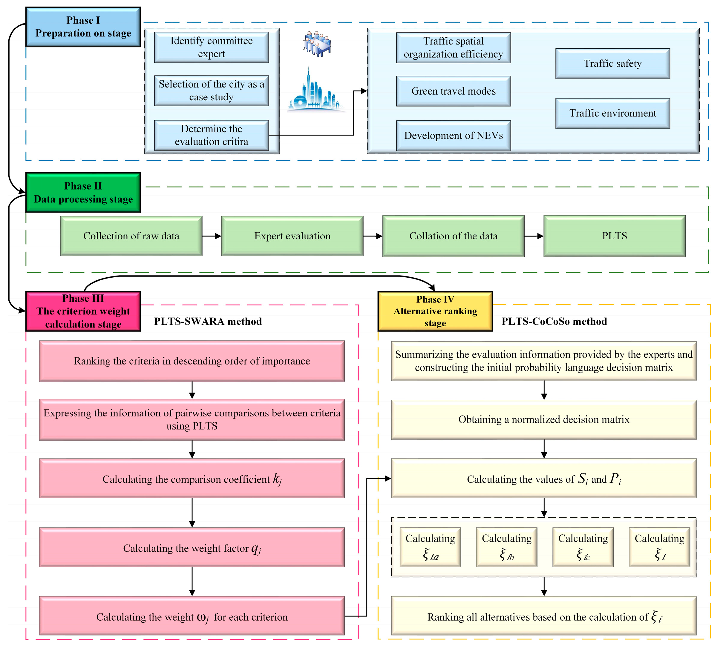
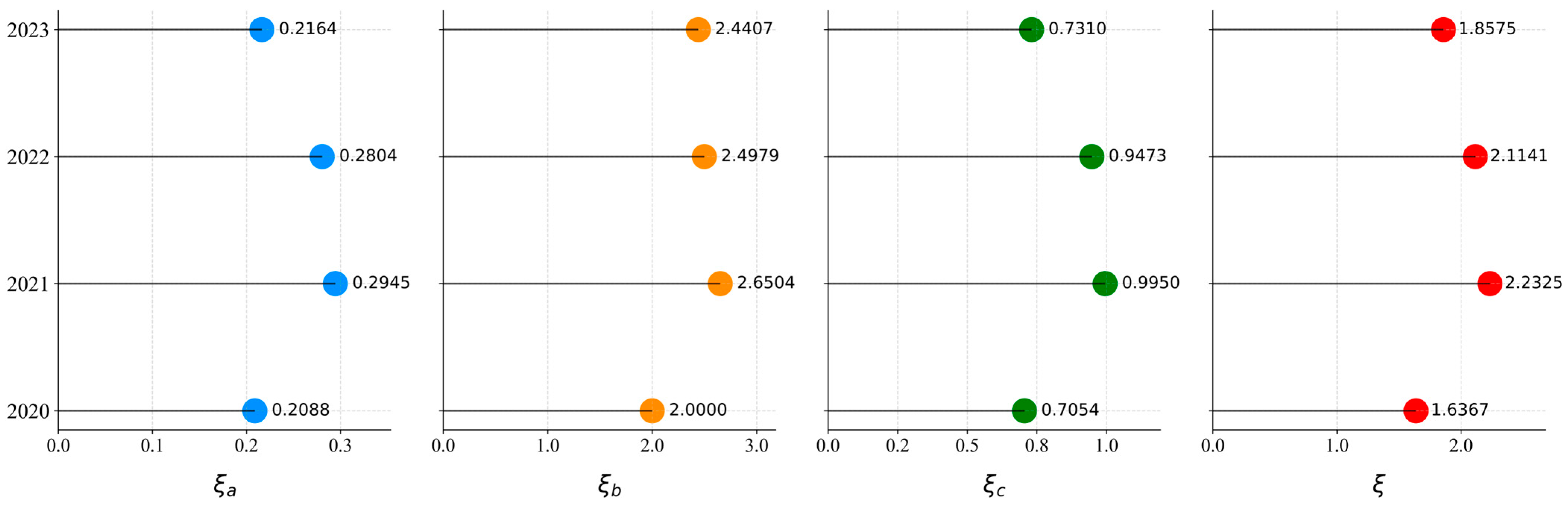
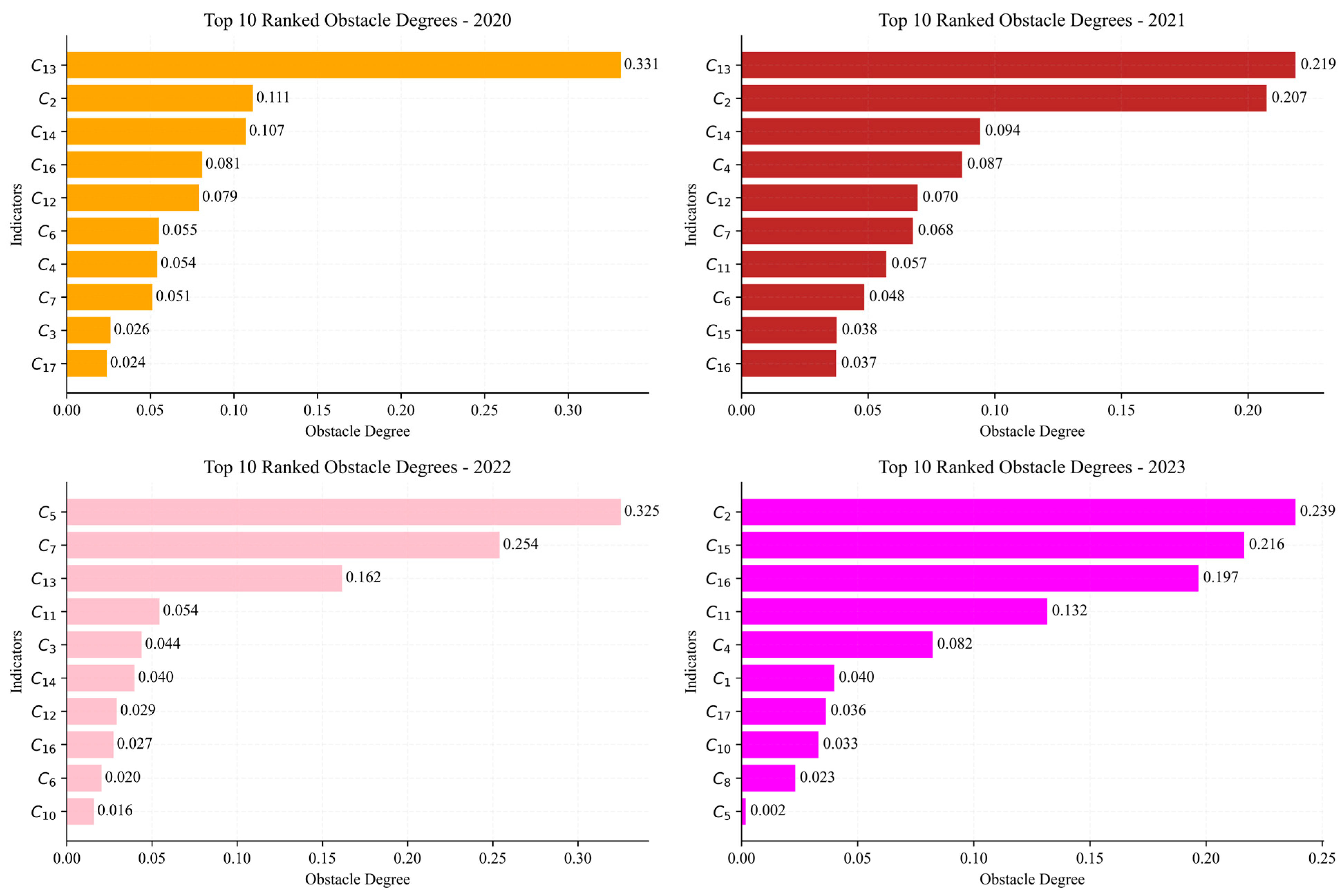
The following sections are organized as follows: Section 2 constructs the evaluation indicator system for the UGTDL; Section 3 establishes the PLTS-based SWARA-CoCoSo evaluation model; Section 4 calculates the UGTDL of Guangzhou from 2020 to 2023 as a case study and verifies the effectiveness and stability of the model through sensitivity analysis; Section 5 analyzes Guangzhou’s green transportation development status and proposes policy recommendations; Section 6 summarizes the paper and provides the future research directions.

2. The UGTDL Evaluation Index System

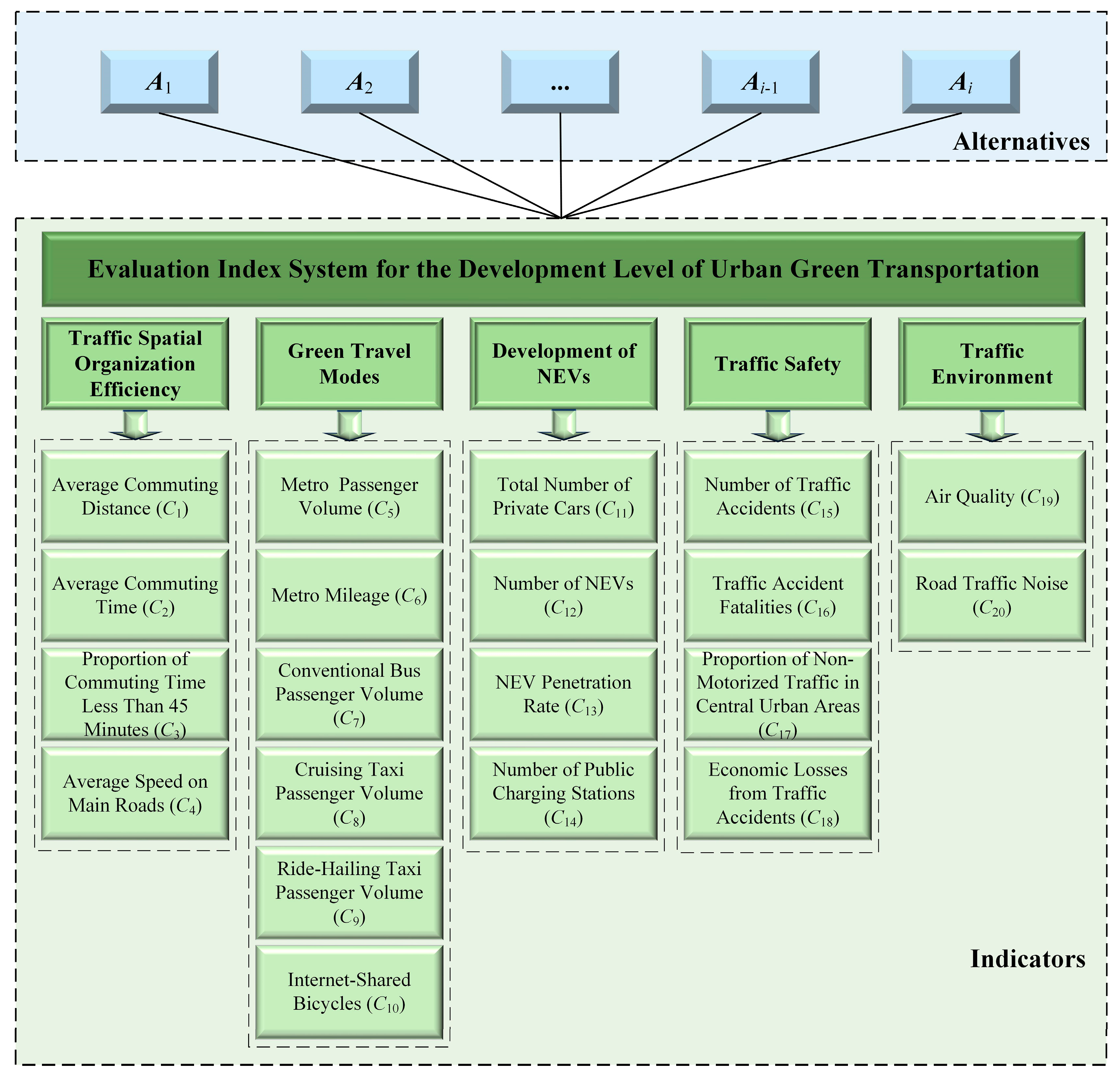
The existing studies on the UGTDL evaluation systems typically focus on the macro-level indicators, such as the urban GDP, carbon emissions, transportation infrastructure development, and public transportation systems [2,3,4,5,6,7,8,9]. However, these studies often neglect the micro-level indicators, such as citizens’ green travel habits and urban commuting conditions, which somewhat limits the comprehensiveness and accuracy of the evaluation systems. Therefore, based on the existing research and incorporating the micro-level indicators, a new UGTDL evaluation index system is proposed. This system consists of five primary indicators: transportation spatial organization efficiency, green travel, the development of NEVs, transportation safety, and the transportation environment (as shown in Figure 1). Each primary indicator is further subdivided into several secondary indicators, which are elaborated in detail below.

2.1. Traffic Spatial Organization Efficiency

The traffic spatial organization efficiency is reflected through four core indicators: average commuting distance ($C_1$), average commuting time ($C_2$), proportion of commuting within 45 min ($C_3$), and average speed on main roads ($C_4$).

The average commuting distance refers to the straight-line distance from the residence to the workplace (or school) for urban commuters, reflecting the rationality of the spatial layout of residential and employment areas in the city. According to the “2024 China Major Cities Commuting Monitoring Report” jointly released by the China Academy of Urban Planning and Design and Baidu Maps, a commuting distance within 5 km is defined as “happy commuting” [42]. The average commuting time measures the time required for residents’ daily commute, influenced by factors such as city size, population density, and transportation modes. Generally, commuting times over 60 min are considered “extreme commuting”, which significantly affects residents’ quality of life [42]. The proportion of commuting within 45 min measures the proportion of trips made within a reasonable commuting time (≤45 min). According to New York 2040—Planning a Strong and Just City, a 90% commuting rate within 45 min is an important standard for evaluating a city’s fairness and sustainable development [43]. Finally, the average speed on main roads refers to the average traffic speed on the primary and secondary roads in the core urban area during the evening peak hours, reflecting the road capacity during commuting rush hours. The level of congestion increases significantly during peak times, and this indicator is used to assess the operational efficiency of urban road traffic.

2.2. Green Travel Modes

Green travel modes are assessed using six indicators: metro passenger volume ($C_5$), metro mileage ($C_6$), conventional bus passenger volume ($C_7$), cruising taxi passenger volume ($C_8$), ride-hailing taxi passenger volume ($C_9$), and internet-shared bicycles ($C_{10}$).

The metro passenger volume reflects the actual passenger capacity of the metro as the core mode of urban public transportation. Due to its high punctuality and stable operations, the metro is a preferred choice for commuters. Complementing this, metro mileage measures the coverage of the metro system and reflects the accessibility of public transportation. The economies of scale in metro networks become apparent once the system reaches a certain size, which in turn enhances its attractiveness for commuting. The conventional bus passenger volume reflects the actual carrying capacity of urban surface public transportation. As the main low-cost travel option for residents, the number of buses and the coverage of bus routes directly affect the variation in this indicator. The cruising taxi passenger volume evaluates the traditional taxi service that supplements public transport, though it is often subject to peak-hour imbalances due to the tidal nature of urban flows. In contrast, the ride-hailing taxi passenger volume reflects the growing adoption of app-based, algorithm-driven transport services that offer improved matching between supply and demand. Lastly, regarding the internet-shared bicycles as a “last mile” solution for public transportation [44], the share of internet-shared bicycles has been increasing in short-distance travel. This mode is convenient, environmentally friendly, and aligns with the development trend of green transportation.

2.3. Development of NEVs

The development and adoption of NEVs are measured by reference to four indicators: the total number of private cars ($C_{11}$), number of NEVs ($C_{12}$), NEV penetration rate ($C_{13}$), and the number of public charging stations ($C_{14}$).

The total number of private cars reflects the degree of private motorization, which is directly linked to road congestion and environmental pressure. The number of NEVs quantifies the scale of clean-energy vehicle adoption, aligned with the national policies for pollution and carbon emission reduction [45]. The NEV penetration rate, defined as the share of NEVs among all motor vehicles, serves as a direct measure of the greening of the urban transport fleet. Supporting infrastructure is captured by the number of public charging stations, which directly affects the convenience, usability, and continued growth of NEV ownership across the city.

2.4. Traffic Safety

Urban traffic safety is evaluated through four key indicators: the number of traffic accidents ($C_{15}$), traffic accident fatalities ($C_{16}$), proportion of non-motorized transport in central urban areas ($C_{17}$), and economic losses from traffic accidents ($C_{18}$).

The number of traffic accidents represents the overall frequency of safety incidents on city roads, while traffic accident fatalities focus on the severity of such incidents in terms of human loss [46]. The proportion of non-motorized transport in central urban areas reflects the extent to which residents adopt walking, cycling, or electric bike modes in high-density districts, which also indicates the city’s progress in promoting active and sustainable mobility. Finally, the economic losses from traffic accidents quantify the total costs resulting from road incidents, including vehicle damage, healthcare expenses, and broader social and economic impacts.

2.5. Traffic Environment

The impact of transportation on the urban environment is assessed through two indicators: the air quality ($C_{19}$) and road traffic noise ($C_{20}$).

The air quality indicator measures the contribution of transport emissions to urban air pollution, a problem intensified by a high vehicle density and poor fuel standards [47]. Despite being influenced by multiple sources, vehicle exhaust remains a dominant factor. The road traffic noise indicator captures the level of acoustic pollution caused by urban road traffic, which directly affects residents’ quality of life and is a key environmental constraint in the development of green transportation systems.

3. Methodology

The SWARA and CoCoSo methods are extended using the PLTS to develop a new evaluation model for the UGTDL. The framework for implementing the model is shown in Figure 2, and the specific concepts and implementation steps will be detailed in this section.

3.1. PLTS

A PLTS is a collection of semantics and their corresponding probabilities, representing the semantic evaluation information expressed by experts using probabilistic linguistic terms. This term set not only captures the uncertainty of experts during the evaluation process but also reflects their preferences. Compared to other semantic evaluation methods, it can avoid the loss of expert preference information during the evaluation process.

Definition 1

([48]).  Let $S=\{s_0,\cdots ,s_{\alpha }\}$ be an LTS. A PLTS is defined as:

$$L(P)=\{L^{(x)}(p^{(x)})|L^{(x)}\in S,p^{(x)}\ge 0,x=1,2,\cdots ,\#L(p),{\displaystyle \sum _{x=1}^{\#L(p)}{p}^{(x)}\le 1}\}$$

(1)

where  $L^{(x)}(p^{(x)})$ denotes that the probability of  $L^{(x)}$ is  $p^{(x)}$ , and  $\#L(p)$ is the number of semantic elements contained in  $L(p)$.

Let the LTS be a language term set with five granularity levels $S^5=\{S_0=VL,S_1=L,S_2=M,S_3=H,S_4=VH\}$. When the expert panel evaluates that an alternative’s performance under a certain criterion is “significantly influential most of the time, occasionally with a moderate influence”, this is recorded as “significantly influential most of the time” denoted as $S_4$ with a probability of 0.8, and “occasionally with moderate influence” denoted as $S_2$ with a probability of 0.1. Thus, the $L(p)=\{(S_4,0.8),(S_2,0.1)\}$.

Let $L{(p)}_1$ and $L{(p)}_2$ be two PLTSs, where:

$$\begin{array}{l}L{(p)}_1=\left.\{L_1^{(x)}(p_1^{(x)})\right|x=1, 2, \dots , \#L{(p)}_1\}\\ L{(p)}_2=\{\left.L_2^{(x)}(p_2^{(x)})\right|x=1, 2, \dots , \#L{(p)}_2\}\end{array}$$

(2)

If $\#L{(p)}_1>\#L{(p)}_2$, it is necessary to add $\#L{(p)}_1-\#L{(p)}_2$ semantic elements to the set $L{(p)}_2$, making the two probabilistic linguistic term sets have the same number of elements. The added semantic elements should be the smallest linguistic terms in the $L{(p)}_2$, with a probability of 0.

Definition 2

([48]). Let ${\displaystyle \sum _{x=1}^{\#L(p)}{p}^{(x)}}<1$, and after normalization, it becomes:

$$\overline{L}(p)=\{\left.L^{(x)}({\overline{p}}^{(x)})\right|x=1, 2, \dots , \#L(p)\}$$

(3)

where  ${\overline{p}}^{(x)}=p^{(x)}/{\displaystyle \sum _{x=1}^{\#L(p)}{p}^{(x)}}$ , and  $L^{(x)}({\overline{p}}^{(x)})$ arranged in ascending order.

Definition 3

([49]). Let $L(p)=\{L^{(x)}(p^{(x)})\left|x=1, 2, \dots , \#L(p)\right.\}$ be a PLTS, and let $r^{\left(x\right)}$ be the subscript of the linguistic term $L^{\left(x\right)}$. The score function of $L(p)$ is defined as:

$$G(L(p))=S_{\overline{\alpha }}$$

(4)

where  $\overline{\alpha }={\displaystyle \sum _{x=1}^{\#L(p)}{r}^{(x)}{p}^{(x)}}/{\displaystyle \sum _{x=1}^{\#L(p)}{p}^{(x)}}$. For PLTSs  $L{(p)}_1$ and  $L{(p)}_2$, if  $G(L{(p)}_1)>G(L{(p)}_2)$, then  $L{(p)}_1>L{(p)}_2$.

Definition 4

([49]). Let $L(p)=\{L^{(x)}(p^{(x)})\left|x=1, 2, \dots , \#L(p)\right.\}$ be a PLTS, and $r^{\left(x\right)}$ be the subscript of the linguistic term $L^{\left(x\right)}$. The score function is $G(L(p))=S_{\overline{\alpha }}$, where  $\overline{\alpha }={\displaystyle {\sum }_{x=1}^{\#L(p)}{r}^{(x)}{p}^{(x)}/}{\displaystyle {\sum }_{x=1}^{\#L(p)}{p}^{(x)}}$, and the deviation degree of $L(p)$ is given by:

$$\sigma (L(p))=({\displaystyle \sum _{x=1}^{\#L(P)}{(p^{(x)}(r^{(x)}-\stackrel{\_}{\alpha }))}^2{)}^{1/2}}/{\displaystyle \sum _{x=1}^{\#L(P)}{p}^{(x)}}$$

(5)

Let  $L{(p)}_1$ and  $L{(p)}_2$ be two PLTSs with score functions  $G(L{(p)}_1)$ and $G(L{(p)}_2)$, and deviation degrees  $\sigma (L{(p)}_1)$ and  $\sigma (L{(p)}_2)$, respectively. When   $G(L{(p)}_1)=G(L{(p)}_2)$, if  $\sigma (L{(p)}_1)<\sigma (L{(p)}_2)$, then  $L{(p)}_1>L{(p)}_2$; if  $\sigma L{(p)}_1=\sigma L{(p)}_2$, then  $L{(p)}_1=L{(p)}_2$; if $\sigma (L{(p)}_1)>\sigma (L{(p)}_2)$, then   $L{(p)}_1<L{(p)}_2$.

Definition 5

([49]).  Let $S=\{s_0,\dots ,s_{\alpha }\}$ be an LTS, and $L(p)=\{L^{(x)}(p^{(x)})\left|x=1, 2,\dots , \#L(p)\right.\}$ be a PLTS. Let $r^{\left(x\right)}$ be the subscript of the linguistic term $L^{\left(x\right)}$. The greater the granularity of the $L^{\left(x\right)}$ in  $L(p)$, the more hesitant the evaluation. The degree of hesitation for  $L(p)$ is given by:

$$H(L(p))={\displaystyle \frac{\frac{1}{\#L(p)}{\displaystyle \sum _{x=1}^{\#L(p)}{(p^{(x)}(r^{(x)}-\overline{\alpha }))}^2}}{\alpha +1}}$$

(6)

Definition 6

([49]).  Let $L(p)=\{L^{(x)}(p^{(x)})\left|x=1, 2,\dots , \#L(p)\right.\}$ be a PLTS. The transformation function that converts  $L(p)$ to an precise value is as follows: 

$$G^{*}(L(p))=\stackrel{\_}{\alpha }-\sigma (L(p))-H(L(p))$$

(7)

As the value of $\overline{\alpha }$ increases, the deviation degree decreases, the hesitation degree decreases, and the probabilistic language term set $L(p)$ becomes more optimal.

3.2. Extended SWARA Method Under the PLTS

The traditional SWARA method determines the subjective weights of indicators by rationally judging the relative importance between adjacent criteria. To improve this method, which does not account for hesitation, uncertainty, and probabilistic information in the evaluation, the SWARA method is extended using probabilistic language as proposed by Pang et al. [24]. This extension ensures the accuracy of the evaluation information. For example, the granularity and meaning of the probabilistic language in the SWARA method are shown in

Table 2. Granularity of PLTS in SWARA.

Granularity	Meaning
0.0	$C_j$  $\mathrm{is}\mathrm{equally}\mathrm{as}\mathrm{important}\mathrm{as}{C}_{j-1}$
0.2	$C_j$  $\mathrm{is}\mathrm{slightly}\mathrm{less}\mathrm{important}\mathrm{than}{C}_{j-1}$
0.4	$C_j$  $\mathrm{is}\mathrm{clearly}\mathrm{less}\mathrm{important}\mathrm{than}{C}_{j-1}$
0.6	$C_j$ is strongly less important than $C_{j-1}$
0.8	$C_j$  $\mathrm{is}\mathrm{extremely}\mathrm{less}\mathrm{important}\mathrm{than}{C}_{j-1}$
1.0	$C_j$  $\mathrm{is}\mathrm{absolutely}\mathrm{less}\mathrm{important}\mathrm{than}{C}_{j-1}$

Note: in this study, granularity is a continuous variable, and the expert panel may use any value within the range as the evaluation granularity.

[27]. The following describes the specific steps for solving the subjective weights of each indicator using the SWARA method extended by using the PLTS.

Step 1: Establish a panel of experts for urban green transportation evaluation. The panel discusses and determines the ordinal relationship of the indicators. Based on the ranking, designate the j-th important indicator as $C_j$, where $C_{j-1}$ is considered more important than $C_j$. The expert panel uses the PLTS to judge the relative importance of adjacent indicators. The judgment results in the PLTS are then converted into precise values using Formulas (5)–(7).

Step 2: Use Formulas (8) and (9) to calculate the coefficient $k_j$ and the weight factor $q_j$, respectively.

$$k_j=\left\{\begin{array}{l}1, j=1\\ G^{*}{(L(p))}_j+1, j>1 \end{array}\right.$$

(8)

$$q_j=\left\{\begin{array}{l}1, j=1\\ {\displaystyle \frac{q_{j-1}}{k_j}}, j>1 \end{array}\right.$$

(9)

Step 3: Calculate the weights of each indicator ${\omega }_j$ according to Formula (10).

$${\omega }_j={\displaystyle \frac{q_j}{{\displaystyle \sum _{j=1}^n{q}_j}}}$$

(10)

3.3. Extended CoCoSo Method Under the PLTS

The CoCoSo method proposed by Yazdani et al. [38] combines a simple additive weighting method with the exponential weighted product model, making it a novel MCDA approach. It can be used for ranking or selecting among various options. By effectively integrating the PLTS with CoCoSo, the granularity of the probabilistic language in CoCoSo is determined. For example, $L(p)=\{(S_6,0.2),(S_7,0.8)\}$ is a PLTS with 9 granularities, represented as “Most of the time, the evaluated object has a high evaluation value on the indicator, but sometimes the evaluation value is slightly higher”, is used, with the specific granularities shown in

Table 3. Granularity of PLTS in CoCoSo.

Granularity	Description
$S_1$	Extremely Low
$S_2$	Very Low
$S_3$	Low
$S_4$	Slightly Low
$S_5$	Average
$S_6$	Slightly High
$S_7$	High
$S_8$	Very High
$S_9$	Extremely High

. The SWARA method and the CoCoSo method are extended in the PLTS environment to determine the weights of the indicators and ultimately calculate the scores and rankings of the alternatives. The specific procedure includes the following five steps [50].

Step 1: Assume that there are $m$ alternatives and $n$ indicators. The evaluation values of the alternatives under each indicator are obtained through discussions within an expert panel, and these values are represented using the PLTS. By using Equations (5)–(7), the PLTSs are converted into precise values, resulting in the initial decision matrix $X$.

$$X={(G^{*}{(L(p))}_{ij})}_{m\times n}=\left[\begin{array}{cccc}{G}^{*}{(L(p))}_{11}& G^{*}{(L(p))}_{12}& \cdots & G^{*}{(L(p))}_{1n}\\ G^{*}{(L(p))}_{21}& G^{*}{(L(p))}_{22}& \cdots & G^{*}{(L(p))}_{2n}\\ ⋮& ⋮& \ddots & ⋮\\ G^{*}{(L(p))}_{m1}& G^{*}{(L(p))}_{m2}& \cdots & G^{*}{(L(p))}_{mn}\end{array}\right]$$

(11)

where $i=1,2,\dots ,m$, $j=1,2,\dots ,n$.

Step 2: The decision matrix $X$ is standardized according to Equations (12) and (13), resulting in the standardized decision matrix $D={(d_{ij})}_{m\times n}$.

$$d_{ij}={\displaystyle \frac{G^{*}{(L(p))}_{ij}-{\min }_j(G^{*}{(L(p))}_{ij})}{{\max }_j(G^{*}{(L(p))}_{ij})-{\min }_j(G^{*}{(L(p))}_{ij})}}, j\in Benefitindicators$$

(12)

$$d_{ij}={\displaystyle \frac{{\max }_j(G^{*}{(L(p))}_{ij})-G^{*}{(L(p))}_{ij}}{{\max }_j(G^{*}{(L(p))}_{ij})-{\min }_j(G^{*}{(L(p))}_{ij})}}, j\in Costindicators$$

(13)

$$D={(d_{ij})}_{m\times n}=\left[\begin{array}{cccc}{d}_{11}& d_{12}& \cdots & d_{1n}\\ d_{21}& d_{22}& \cdots & d_{2n}\\ ⋮& ⋮& \ddots & ⋮\\ d_{m1}& d_{m2}& \cdots & d_{mn}\end{array}\right]$$

(14)

where $i=1,2,\dots ,m$, $j=1,2,\dots ,n$.

Step 3: Calculate the values of $S_i$ and $P_i$. The value of $S_i$ is determined using the grey relational generation method, i.e., Equation (15), while the value of $P_i$ is determined based on the multiplicative properties of Weighted Aggregated Sum Product Assessment (WASPAS), i.e., Equation (16).

$$S_i={\displaystyle \sum _{j=1}^n({\omega }_j}\times d_{ij})$$

(15)

$$P_i={\displaystyle \sum _{j=1}^n(}{d}_{ij}{)}^{{\omega }_j}$$

(16)

where ${\omega }_j$ represents the weight of the indicator j, which is calculated using the PLTS-SWARA method.

Step 4: The relative weights of the alternatives are calculated using the following aggregation strategies. In this step, three evaluation scoring strategies are used to generate the relative weights of the other alternatives, which are derived through Equations (17)–(19).

$${\xi }_{ia}={\displaystyle \frac{P_i+S_i}{{\displaystyle \sum _{i=1}^n(P_i+S_i)}}}$$

(17)

$${\xi }_{ib}={\displaystyle \frac{S_i}{\underset{i}{\min }{S}_i}}+{\displaystyle \frac{P_i}{\underset{i}{\min }{P}_i}}$$

(18)

$${\xi }_{ic}={\displaystyle \frac{\lambda (S_i)+(1-\lambda )(P_i)}{\left(\lambda \underset{i}{\max }{S}_i+(1-\lambda )\underset{i}{\max }{P}_i\right)}};0\le \lambda \le 1$$

(19)

Typically, the value of $\lambda$ in Equation (19) is set to 0.5.

Step 5: The score of each alternative ${\xi }_i$ is calculated according to Equation (20). Based on the principle that a higher ${\xi }_i$ value is better, the ranking of all alternatives is obtained.

$${\xi }_i=\sqrt[3]{{\xi }_{ia}\times {\xi }_{ib}\times {\xi }_{ic}}+{\displaystyle \frac{{\xi }_{ia}+{\xi }_{ib}+{\xi }_{ic}}{3}}$$

(20)

4. Case Study

4.1. Case Introduction

This study is based on data from 2020 to 2023, focusing on Guangzhou as the research subject. It analyzes the UGTDL in the city, while exploring the driving forces and obstacles behind this process. As the capital of Guangdong Province and a national central city, Guangzhou ranks among the top Chinese cities in terms of GDP—specifically, it ranked 4th nationwide in 2020, 2021, and 2023, and 5th in 2022. This consistently high economic performance underscores its leading role in southern China’s economic growth. By the end of 2023, the city’s permanent population had reached 18.83 million. As a megacity, Guangzhou ranks at the forefront nationwide in terms of urban scale, population density, and GDP. The city’s geographic advantages and industrial foundation make it an ideal location for the application of NEVs. However, as a megacity, Guangzhou faces greater challenges in promoting the transformation to green transportation, including issues such as traffic congestion, complex travel demands, and pressure on infrastructure construction. Therefore, the experiences and challenges faced by Guangzhou in its transition to green transportation offer valuable lessons for other major cities in China and globally. Data from the period of 2020–2023 were selected to analyze the rapid development and widespread adoption of NEVs in China, particularly in the context of NEV promotion, highlighting the characteristics exhibited in the development of urban green transportation during this period.

4.2. Implementation and Computation

All computations and modeling tasks in this study were carried out using Python 3.12.4. The main Python packages used included numpy, pandas, pymcdm, and matplotlib.

In this study, a group of five experts from the field of transportation were invited to form an expert panel. The panel discussed and evaluated the importance of the 20 indicators in the urban green transportation evaluation index system shown in Figure 1, and then ranked the indicators in descending order of importance. The indicators were compared pairwise, with comparison values represented using the PLTS. The PLTS values were then converted to precise values using Equations (5)–(7). The coefficient $k_j$ was calculated using Equation (8). The weight factor $q_j$ was computed using Equation (9). The weight of each indicator ${\omega }_j$ was then determined using Equation (10). The specific results are shown in

Table 4. Weight calculation results for each indicator based on the PLTS-SWARA method.

${\mathit{C}}_{\mathit{j}}$	L(p)j	G*(L(p))j	kj	Qj	ωj
$C_{13}$	/	/	1.0000	1.0000	0.1796
$C_5$	$\{S_{0.1}(0.3),S_{0.2}(0.6)\}$	0.1381	1.1381	0.8786	0.1578
$C_7$	$\{S_{0.2}(0.3),S_{0.4}(0.7)\}$	0.2800	1.2800	0.6864	0.1233
$C_2$	$\{S_{0.4}(0.2),S_{0.5}(0.6)\}$	0.4484	1.4484	0.4739	0.0851
$C_{15}$	$\{S_{0.1}(0.6),S_{0.2}(0.3)\}$	0.1019	1.1019	0.4301	0.0773
$C_{16}$	$\{S_{0.1}(0.7),S_{0.2}(0.3)\}$	0.1002	1.1002	0.3909	0.0702
$C_{14}$	$\{S_{0.2}(0.5),S_{0.3}(0.3)\}$	0.2101	1.2101	0.3231	0.0580
$C_{11}$	$\{S_{0.2}(0.3),S_{0.3}(0.6)\}$	0.2350	1.2350	0.2616	0.0470
$C_{11}$	$\begin{array}{c}\{S_{0.1}(0.8),S_{0.2}(0.2)\}\end{array}$	0.0973	1.0973	0.2384	0.0428
$C_4$	$\{S_{0.2}(0.8),S_{0.3}(0.2)\}$	0.1973	1.1973	0.1991	0.0358
$C_6$	$\{S_{0.2}(0.6),S_{0.3}(0.2)\}$	0.1984	1.1984	0.1661	0.0298
$C_3$	$\{S_{0.4}(0.7),S_{0.5}(0.2)\}$	0.3978	1.3978	0.1189	0.0214
$C_1$	$\{S_{0.5}(0.6),S_{0.6}(0.2)\}$	0.4984	1.4984	0.0793	0.0143
$C_{17}$	$\{S_{0.1}(0.7),S_{0.2}(0.2)\}$	0.0978	1.0978	0.0723	0.0130
$C_{10}$	$\{S_{0.1}(0.7),S_{0.2}(0.1)\}$	0.0970	1.0970	0.0659	0.0118
$C_9$	$\{S_{0.1}(0.6),S_{0.2}(0.3)\}$	0.1019	1.1019	0.0598	0.0107
$C_8$	$\{S_{0.3}(0.7),S_{0.4}(0.3)\}$	0.3002	1.3002	0.0460	0.0083
$C_{19}$	$\{S_{0.4}(0.5),S_{0.6}(0.5)\}$	0.4285	1.4285	0.0322	0.0058
$C_{18}$	$\begin{array}{c}\{S_{0.3}(0.7),S_{0.4}(0.3)\}\end{array}$	0.3002	1.3002	0.0248	0.0044
$C_{20}$	$\begin{array}{c}\{S_{0.3}(0.6),S_{0.4}(0.2)\}\end{array}$	0.2984	1.2984	0.0191	0.0034

.

Subsequently, based on the evaluation index system of the UGTDL, the raw data for all evaluation indicators of Guangzhou from 2020 to 2023 were collected (the data were mainly sourced from the respective years’ Guangzhou Statistical Yearbook and Statistical Reports). The expert panel further discussed the original data and obtained the evaluation values for Guangzhou in each green transportation evaluation indicator $C_j$ from 2020 to 2023, represented using a PLTS, as shown in

Table 5. Evaluation information table based on PLTS.

	$C_1$	$C_2$	$C_3$	$C_4$	$C_5$
A2020	$\{S_5(0.9)\}$	$\{S_6(0.9)\}$	$\{S_4(0.9)\}$	$\{S_5(0.8)\}$	$\{S_5(0.8)\}$
A2021	$\{S_5(0.9)\}$	$\{S_7(0.7)\}$	$\{S_5(0.9)\}$	$\{S_4(0.2),S_5(0.8)\}$	$\{S_5(0.9)\}$
A2022	$\{S_3(0.4),S_4(0.6)\}$	$\{S_3(0.2),S_4(0.8)\}$	$\{S_3(0.9)\}$	$\{S_7(0.8)\}$	$\{S_2(0.5),S_3(0.5)\}$
A2023	$\{S_6(0.8)\}$	$\{S_7(0.8)\}$	$\{S_6(0.9)\}$	$\{S_5(0.8)\}$	$S_5(0.7),S_6(0.3)$
	$C_6$	$C_7$	$C_8$	$C_9$	$C_{10}$
A2020	$\{S_5(0.8)\}$	$\{S_5(0.9)\}$	$\{S_4(0.3),S_5(0.7)\}$	$\{S_4(0.8)\}$	$\{S_5(0.8)\}$
A2021	$\{S_6(0.8)\}$	$\{S_5(0.8)\}$	$\{S_5(0.8)\}$	$\{S_5(0.8)\}$	$\{S_7(0.8)\}$
A2022	$\{S_7(0.8)\}$	$\{S_1(0.2),S_2(0.8)\}$	$\{S_4(0.8)\}$	$\{S_6(0.8)\}$	$\{S_4(0.3),S_5(0.7)\}$
A2023	$\{S_8(0.8)\}$	$\{S_6(0.9)\}$	$\{S_3(0.9)\}$	$\{S_7(0.7)\}$	$\{S_3(0.8)\}$
	$C_{11}$	$C_{12}$	$C_{13}$	$C_{14}$	$C_{15}$
A2020	$\{S_5(0.8)\}$	$\{S_3(0.8)\}$	$\{S_3(0.9)\}$	$\{S_2(0.9)\}$	$\{S_4(0.5),S_5(0.5)\}$
A2021	$\{S_6(0.8)\}$	$\{S_4(0.8)\}$	$\{S_4(0.9)\}$	$\{S_4(0.9)\}$	$\{S_5(0.9)\}$
A2022	$\{S_6(0.5),S_7(0.5)\}$	$\{S_5(0.8)\}$	$\{S_4(0.5),S_5(0.5)\}$	$\{S_6(0.9)\}$	$\{S_4(0.8)\}$
A2023	$\{S_7(0.7)\}$	$\{S_6(0.7)\}$	$\{S_5(0.9)\}$	$\{S_8(0.9)\}$	$\{S_6(0.8)\}$
	$C_{16}$	$C_{17}$	$C_{18}$	$C_{19}$	$C_{20}$
A2020	$\{S_6(0.5),S_7(0.5)\}$	$\{S_3(0.8)\}$	$\{S_5(0.8)\}$	$\{S_6(0.8)\}$	$\{S_5(0.8)\}$
A2021	$\{S_4(0.7)\}$	$\{S_6(0.5),S_7(0.5)\}$	$\{S_3(0.8)\}$	$\{S_5(0.8)\}$	$\{S_5(0.7)\}$
A2022	$\{S_3(0.8)\}$	$\{S_7(0.8)\}$	$\{S_4(0.8)\}$	$\{S_4(0.8)\}$	$\{S_4(0.5),S_5(0.5)\}$
A2023	$\{S_8(0.9)\}$	$\{S_6(0.4),S_7(0.6)\}$	$\{S_3(0.8)\}$	$\{S_7(0.8)\}$	$S_5\{(0.9)\}$

. The PLTS values were converted into precise values using Equations (5)–(7), resulting in the initial decision matrix, as shown in

Table 6. Initial decision matrix $X$.

	$C_1$	$C_2$	$C_3$	$C_4$	$C_5$
A2020	5	6	4	5	5
A2021	5	7	5	4.5652	5
A2022	3.2414	3.5652	3	7	2.1256
A2023	6	7	6	5	4.9883
	$C_6$	$C_7$	$C_8$	$C_9$	$C_{10}$
A2020	5	5	4.3883	4	5
A2021	6	5	5	5	7
A2022	7	1.5652	4	6	4.3883
A2023	8	6	3	7	3
	$C_{11}$	$C_{12}$	$C_{13}$	$C_{14}$	$C_{15}$
A2020	5	3	3	2	4.1256
A2021	6	4	4	4	5
A2022	6.1256	5	4.1256	6	4
A2023	7	6	5	8	6
	$C_{16}$	$C_{17}$	$C_{18}$	$C_{19}$	$C_{20}$
A2020	6.1256	3	5	6	5
A2021	4	6.1256	3	5	5
A2022	3	7	4	4	4.1256
A2023	8	6.2414	3	7	5

. Since indicators $C_1$, $C_2$, $C_{11}$, $C_{15}$, $C_{16}$, and $C_{18}$ belong to cost-type indicators, while the other indicators are benefit-type indicators, Equations (12) and (13) were used to standardize the benefit-type and cost-type indicators in Table 6, respectively, resulting in a standardized decision matrix $D$, as shown in

Table 7. Standardized decision matrix $D$.

	$C_1$	$C_2$	$C_3$	$C_4$	$C_5$
A2020	0.3625	0.2911	0.3333	0.1786	1.0000
A2021	0.3625	0.0000	0.6667	0.0000	1.0000
A2022	1.0000	1.0000	0.0000	1.0000	0.0000
A2023	0.0000	0.0000	1.0000	0.1786	0.9959
	$C_6$	$C_7$	$C_8$	$C_9$	$C_{10}$
A2020	0.0000	0.7745	0.6942	0.0000	0.5000
A2021	0.3333	0.7745	1.0000	0.3333	1.0000
A2022	0.6667	0.0000	0.5000	0.6667	0.3471
A2023	1.0000	1.0000	0.0000	1.0000	0.0000
	$C_{11}$	$C_{12}$	$C_{13}$	$C_{14}$	$C_{15}$
A2020	1.0000	0.0000	0.0000	0.0000	0.9372
A2021	0.5000	0.3333	0.5000	0.3333	0.5000
A2022	0.4372	0.6667	0.5628	0.6667	1.0000
A2023	0.0000	1.0000	1.0000	1.0000	0.0000
	$C_{16}$	$C_{17}$	$C_{18}$	$C_{19}$	$C_{20}$
A2020	0.3749	0.0000	0.0000	0.6667	0.0000
A2021	0.8000	0.7814	1.0000	0.3333	0.0000
A2022	1.0000	1.0000	0.5000	0.0000	1.0000
A2023	0.0000	0.8104	1.0000	1.0000	0.0000

.

Then, the weighted comparable sequence $S_i$ and the power-weighted comparable sequence $P_i$ were determined using Formulas (15) and (16) in the CoCoSo method, with the results shown in

Table 8. Calculation of the value of $S_i$.

	$C_1$	$C_2$	$C_3$	$C_4$	$C_5$	$C_6$	$C_7$
A2020	0.0052	0.0248	0.0071	0.0064	0.1578	0.0000	0.0955
A2021	0.0052	0.0000	0.0142	0.0000	0.1578	0.0099	0.0955
A2022	0.0143	0.0851	0.0000	0.0358	0.0000	0.0199	0.0000
A2023	0.0000	0.0000	0.0214	0.0064	0.1572	0.0298	0.1233
	$C_8$	$C_9$	$C_{10}$	$C_{11}$	$C_{12}$	$C_{13}$	$C_{14}$
A2020	0.0057	0.0000	0.0059	0.0470	0.0000	0.0000	0.0000
A2021	0.0083	0.0036	0.0118	0.0235	0.0143	0.0898	0.0193
A2022	0.0041	0.0072	0.0041	0.0205	0.0286	0.1011	0.0387
A2023	0.0000	0.0107	0.0000	0.0000	0.0428	0.1796	0.0580
	$C_{15}$	$C_{16}$	$C_{17}$	$C_{18}$	$C_{19}$	$C_{20}$	$S_i$
A2020	0.0724	0.0263	0.0000	0.0000	0.0039	0.0000	0.4581
A2021	0.0386	0.0562	0.0101	0.0044	0.0019	0.0000	0.5647
A2022	0.0773	0.0702	0.0130	0.0022	0.0000	0.0034	0.5255
A2023	0.0000	0.0000	0.0105	0.0044	0.0058	0.0000	0.6501

and

Table 9. Calculation of the value of $P_i$.

	$C_1$	$C_2$	$C_3$	$C_4$	$C_5$	$C_6$	$C_7$
A2020	0.9856	0.9003	0.9768	0.9402	1.0000	0.0000	0.9690
A2021	0.9856	0.0000	0.9914	0.0000	1.0000	0.9677	0.9690
A2022	1.0000	1.0000	0.0000	1.0000	0.0000	0.9880	0.0000
A2023	0.0000	0.0000	1.0000	0.9402	0.9994	1.0000	1.0000
	$C_8$	$C_9$	$C_{10}$	$C_{11}$	$C_{12}$	$C_{13}$	$C_{14}$
A2020	0.9970	0.0000	0.9918	1.0000	0.0000	0.0000	0.0000
A2021	1.0000	0.9883	1.0000	0.9680	0.9540	0.8829	0.9382
A2022	0.9943	0.9957	0.9876	0.9619	0.9828	0.9019	0.9767
A2023	0.0000	1.0000	0.0000	0.0000	1.0000	1.0000	1.0000
	$C_{15}$	$C_{16}$	$C_{17}$	$C_{18}$	$C_{19}$	$C_{20}$	$P_i$
A2020	0.9950	0.9334	0.0000	0.0000	0.9977	0.0000	11.6868
A2021	0.9479	0.9845	0.9968	1.0000	0.9937	0.0000	16.5679
A2022	1.0000	1.0000	1.0000	0.9969	0.0000	1.0000	15.7857
A2023	0.0000	0.0000	0.9973	1.0000	1.0000	0.0000	11.9369

. The comprehensive evaluation scores ${\xi }_{ia}$, ${\xi }_{ib}$, and ${\xi }_{ic}$, were calculated based on Formulas (17)–(19). To calculate the scores for the years under evaluation, we used Formula (20) to obtain the value of $\xi$. The calculation results for all the parameters and rankings are detailed in

Table 10. Calculation results of Guangzhou’s UGTDL based on the PLTS-SWARA-CoCoSo model.

	${\mathit{\xi }}_{\mathit{a}}$	Rank	${\mathit{\xi }}_{\mathit{b}}$	Rank	${\mathit{\xi }}_{\mathit{c}}$	Rank	$\mathit{\xi }$	Final Rank
A2020	0.2088	4	2.0000	4	0.7054	4	1.6367	4
A2021	0.2945	1	2.6504	1	0.9950	1	2.2325	1
A2022	0.2804	2	2.4979	2	0.9473	2	2.1141	2
A2023	0.2164	3	2.4407	3	0.7310	3	1.8575	3

. At this point, the calculation process of Guangzhou’s UGTDL, based on the 20 evaluation indicators and the PLTS-SWARA-CoCoSo model, has been fully provided. According to the results obtained, A₂₀₂₁ > A₂₀₂₂ > A₂₀₂₃ > A₂₀₂₀, which shows that the UGTDL in Guangzhou was the lowest in 2020. With the promotion of NEVs, there was a leap in the city’s UGTDL in 2021, but it decreased consecutively in 2022 and 2023. Figure 3 shows the ranking trends of Guangzhou’s UGTDL from 2020 to 2023 based on various parameter indicators.

4.3. Sensitivity Analysis

This section explores the impact of fluctuations in the indicator weights on the UGTDL scores and rankings, and verifies the reliability of the model through sensitivity analysis. The weights of indicator $C_j$ were adjusted upward and downward by 10%, 20%, and 30% based on the original weights calculated using the PLTS-SWARA method. As the weight of $C_j$ changed, the weights of the other indicators were also adjusted accordingly to ensure that the sum of all the indicator weights equaled 1. Based on the above weight adjustment principles, the sensitivity analysis results for 140 different scenarios, corresponding to 20 indicators and seven weight schemes, were calculated. These results are illustrated in Figure 4.

As shown in Figure 4, it can be observed that, first, fluctuations in the indicator weights within the range of 0.7, 0.8, 0.9, 1.0, 1.1, and 1.2 did not affect the ranking results of the UGTDL evaluation in Guangzhou from 2020 to 2023, with the ranking always remaining as A₂₀₂₁ > A₂₀₂₂ > A₂₀₂₃ > A₂₀₂₀. This indicated that the calculation results of the proposed urban green transportation development evaluation model were highly stable and reliable.

Second, when the indicator weights changed, the scores for the urban green transportation development level in 2020 and 2021 showed minimal changes and remained very stable, while in 2022 and 2023, although the rankings remained unchanged, the scores experienced significant fluctuations.

Finally, it can be observed that changes in $C_2$, $C_5$, $C_{11}$, $C_{12}$, $C_{13}$, $C_{14}$, $C_{15}$, and $C_{16}$ noticeably influenced the score changes in 2022 and 2023, indicating that these factors were the key influences on the UGTDL in Guangzhou over the past two years.

5. Evaluation Analysis and Recommendations

5.1. Evaluation Analysis

In order to further analyze the constraints affecting the UGTDL in Guangzhou from 2020 to 2023, and to provide direction for the future development of the urban transportation in Guangzhou, the obstacle degree model [45] was used to calculate the top ten obstacle degree indicators for the green transportation development in Guangzhou from 2020 to 2023 (as shown in Figure 5). The specific analysis was as follows.

5.1.1. The Analysis of Traffic Spatial Organization Efficiency

According to the obstacle degree analysis in Figure 5, the $C_2$ ranked second in both 2020 and 2021, but by 2023, it became the highest obstacle degree. However, in 2022, this indicator did not appear in the top ten obstacle rankings, as the average commuting time significantly decreased in that year. The $C_4$ is highly correlated with $C_2$. In 2020, 2021, and 2023, the road speed was one of the top ten obstacle factors, while its ranking dropped in 2022. The data show that the road speed in 2022 significantly improved compared to the other years. This suggests that the average commuting time is a core factor influencing the urban green transportation development and has an inverse relationship with the road speed.

5.1.2. The Analysis of Green Travel Modes

In 2020 and 2021, under the first-level indicator of green travel modes, two second-level indicators were in the top ten obstacle degree rankings, namely $C_6$ and $C_7$. In 2022, four second-level indicators under the green travel first-level indicator appeared in the top ten obstacle degree rankings ($C_5$, $C_6$, $C_7$, $C_{10}$), with $C_5$ ranking first in obstacle degree. This was because the metro passenger volume in that year was the lowest among the four years. By 2023, $C_6$ and $C_7$ were no longer in the top ten obstacle degree rankings. However, $C_{10}$ were an obstacle degree factor in both 2022 and 2023.

5.1.3. The Analysis of Development of NEVs

In 2020, 2021, and 2022, nearly all the second-level indicators under the first-level indicator of NEV development appeared in the top ten obstacle degree rankings (2020: $C_{12}$, $C_{13}$, $C_{14}$; 2021: $C_{11}$, $C_{12}$, $C_{13}$, $C_{14}$; 2022: $C_{11}$, $C_{12}$, $C_{13}$, $C_{14}$). The $C_{13}$ and the $C_{14}$ ranked first and third, respectively, in 2020 and 2021. However, by 2022, the rankings of these two indicators significantly dropped to third and sixth, respectively. With the increase in the penetration rate of NEVs and the number of charging piles, by 2023, only the $C_{11}$ remained as the only second-level indicator under this first-level indicator in the top ten obstacle degree rankings.

5.1.4. The Analysis of Traffic Safety and Traffic Environment

From 2020 to 2023, the traffic environment indicators never appeared in the top ten obstacle degree rankings. However, the $C_{16}$ consistently ranked as a top-ten obstacle in all four years. In 2021 and 2022, the obstacle degree of $C_{16}$ was relatively low. In contrast, in 2020 and 2023, the obstacle degree of $C_{16}$ ranked higher, being fourth and third, respectively. In 2023, $C_{15}$ ranked second in the obstacle degree rankings. In the two years when $C_{16}$ ranked higher (2020 and 2023), $C_{17}$ also appeared in the top ten obstacle degree rankings. This indicates that the traffic safety has a significant impact on the UGTDL.

5.2. Analysis Discussion

5.2.1. Discussion of the Research Results

Based on the comprehensive evaluation results and obstacle factor analysis, several core insights into Guangzhou’s urban green transportation development level (UGTDL) from 2020 to 2023 can be derived:

(1)

The average commuting time serves as a core constraint reflecting the overall efficiency of the urban traffic spatial organization. In all the years except 2022, this indicator consistently appeared among the top obstacle factors. Its performance is closely tied to the average road speed, with longer commuting times reflecting systemic congestion or inefficiencies. The sharp drop in this indicator in 2022—coinciding with a significant rise in the average road speed—demonstrates how infrastructure optimization and operational improvements can have immediate positive effects on the UGTDL. Therefore, the traffic spatial layout and commuting efficiency remain foundational to sustainable transportation development.

(2)

The role of diversified green travel modes has become increasingly prominent. In particular, the utilization of metro systems, internet-shared bicycles, and non-motorized travel options showed strong correlations with the UGTDL rankings, especially in 2022. When the metro passenger volume declined that year, the related indicators quickly emerged as the key obstacles. This suggests that beyond the infrastructure presence, user adoption and system integration (e.g., metro–bus–bike connectivity) are critical to maintaining momentum in the green transportation uptake.

(3)

The development of NEVs has played a catalytic but gradually saturating role. From 2020 to 2021, NEV-related indicators (number of NEVs, penetration rate, number of charging stations) were among the top contributors to the UGTDL growth. However, from 2022 onward, their marginal utility declined. This indicates a typical diffusion pattern in green technology adoption, where early-stage growth is rapid but later stages demand deeper systemic integration (e.g., intelligent mobility, multi-modal sharing, battery recycling systems) to sustain value creation.

(4)

Traffic safety is a persistent structural obstacle and a crucial foundation for green transportation. Indicators like traffic accident fatalities and the total number of accidents appeared repeatedly in the obstacle rankings, particularly in 2020 and 2023. Despite the technological advancements and improved infrastructure, safety risks remain a deterrent to modal shift, especially toward vulnerable travel forms such as cycling and walking. This underscores the need for a “people-centered” planning philosophy that prioritizes the protection of vulnerable road users through improved infrastructure, monitoring systems, and public education.

5.2.2. Discussion of Research Innovation

The methods applied in the research on green transportation development evaluation in existing cities include AHP, the entropy weight method, TOPSIS, DEMATEL, and GRA, etc. (Refs. [2,3,4,5,6,7,8,9]). These studies have provided valuable insights into understanding the green transportation trends of specific cities. However, most of these methods heavily rely on unidimensional weighting schemes (e.g., entropy or expert-based methods) or compensatory decision rules (e.g., TOPSIS), which may lead to distorted results when inefficient key indicators are offset by efficient ones. In contrast, the PLTS-SWARA-CoCoSo method overcomes some of these limitations:

(1)

Compared to traditional crisp values or basic fuzzy logic, the PLTS allows experts to express hesitant or uncertain judgments more accurately, capturing the inherent subjectivity and fuzziness in green transportation assessments.

(2)

SWARA ensures that the weighting process is more intuitive, cognitively more economical, and reflects experts’ continuous judgments of importance—something that the entropy method cannot achieve.

(3)

CoCoSo, as a non-compensatory ranking method, enhances the stability and interpretability of the results by preventing poor performance in critical areas (e.g., safety and commuting time) from being unfairly offset by strong performance in other areas (e.g., NEV numbers).

(4)

Furthermore, the sensitivity analysis results further demonstrate the robustness of this model.

5.3. Recommendations

To enhance the UGTDL, the following recommendations are proposed:

(1)

Optimize the urban traffic spatial layout and improve the commuting efficiency. Specifically, traffic management departments should use Intelligent Traffic Systems to monitor and predict the traffic flow on major roads in real time, dynamically adjust traffic signal timings, and maximize the road capacity to reduce unnecessary travel time. In addition, there should be an active promotion of increasing the share of non-motorized transport in the central urban area, providing more convenient pathways for non-motorized travel, optimizing the traffic environment, and alleviating road congestion.

(2)

Promote diversified green travel modes and improve the green transportation infrastructure. Especially in suburban areas with insufficient public transportation coverage, it is recommended to accelerate the development of shared bicycles, shared electric scooters, and other emerging green travel modes, and improve the related infrastructure and management. At the same time, the public transport network layout, particularly the connectivity between subways and buses, should be further optimized to shorten travel times, enhancing the attractiveness of green travel and reducing the reliance on private cars.

(3)

Accelerate the layout of NEVs and charging facilities, and promote the development of intelligent transportation. As the ownership and penetration rate of NEVs increase year by year, their effectiveness in promoting green transportation development is gradually diminishing. However, their importance in the green transportation system remains significant. Therefore, government policies should continue to support the promotion of NEVs and increase the investment in the construction of charging facilities, especially in public charging stations to address the “charging difficulties” issue. Additionally, it is essential to promote the integration of smart driving technologies with NEVs, advancing the intelligent and digital management of traffic to improve the traffic flow management efficiency and reduce the traffic accidents caused by human factors.

(4)

Enhance the traffic safety and implement a “people-centered” development philosophy. It is recommended that traffic management departments strengthen the safety supervision in high-risk areas and during peak hours, increase the construction of traffic safety infrastructure such as more pedestrian crossings, and install traffic monitoring equipment. In addition, it is crucial to raise the public awareness of traffic safety, improve the safety technology standards, and particularly ensure that the application of intelligent traffic management systems safeguards the safety of all road users, especially vulnerable groups such as pedestrians and cyclists. The human-centered philosophy should be fully integrated into the design, management, and implementation of the entire transportation system.

(5)

Promote green transportation environment construction. The government should strengthen the control of the transportation pollution sources and further promote the adoption of environmentally friendly vehicles such as new energy buses and taxis. Introducing green transportation subsidy policies to encourage citizens to choose environmentally friendly transport options will help reduce pollution emissions at the source and improve the traffic environment. Additionally, increasing the urban greenery coverage and improving the ecological environment around roads can help mitigate traffic noise pollution, enhancing the travel experience and well-being of citizens.

6. Conclusions

This study proposes a UGTDL assessment framework based on the PLTS and SWARA-CoCoSo combined model. By introducing the PLTS model into the assessment system, it effectively addresses the limitations of traditional evaluation methods when dealing with uncertainty and hesitation, thus improving the accuracy of expert evaluation information. For weight distribution, the SWARA method is employed, significantly reducing the computational complexity under high-dimensional indicators while maintaining the rationality of the assessment. The CoCoSo method is used for the comprehensive ranking of the indicators, which not only enhances the computational efficiency but also avoids the compensatory issues in decision making, thereby strengthening the scientific and practical nature of the model.

Using Guangzhou as a case study, this framework successfully evaluates the UGTDL from 2020 to 2023 and verifies the stability and reliability of the model through sensitivity analysis. The evaluation results provide strong support for the optimization of the green transportation policies in Guangzhou, offering practical policy recommendations, particularly in areas such as transportation infrastructure, green travel modes, and the promotion of NEVs.

Importantly, the proposed framework is not city specific and can be readily reproduced in other urban regions. As long as the required multi-dimensional transportation data are available and expert knowledge can be elicited for linguistic evaluation, the PLTS–SWARA–CoCoSo methodology can be applied with minimal modifications. This enhances the generalizability of the study and provides a scalable analytical tool for assessing the UGTDL in different geographic and policy contexts. However, this study also has several limitations. For instance, while the reliance on expert judgment for linguistic evaluation facilitates the quantification of qualitative data, it may lead to excessive subjectivity or difficulties in reaching a consensus among the experts, especially when there are discrepancies in the data quality or variations in experts’ expertise. In addition, due to the data availability constraints, an in-depth analysis of the intra-city disparities in the green transportation development across the districts and counties in Guangzhou, as well as the comparisons between Guangzhou and other cities, has not been explored. Future research could integrate large-scale group decision-making methods to further enhance the evaluation accuracy or collect data from more cities and different periods to conduct spatiotemporal evolution analysis of the UGTDL, thereby providing more comprehensive decision support for the formulation of green transportation policies.

References

1. Dong, Y.; Wang, D.; Zeng, F.; Zhang, Y. A novel MADM model integrating hybrid information for evaluating the development prospects of urban new energy vehicles. PLoS ONE 2025, 20, e0314026. [Google Scholar] [CrossRef] [PubMed]
2. Wang, M.; Lin, X.; Yu, L. Comprehensive evaluation of green transportation in Chongqing main urban area based on sustainable development theory. Syst. Sci. Control Eng. 2019, 7, 369–378. [Google Scholar] [CrossRef]
3. Wang, Q.; Qian, Y.; Zeng, J.; Guang, X. Research on evaluation of green transportation development in valley city under the background of new urbanization: Taking lanzhou as an example. Ecol. Econ. 2020, 36, 95–99. [Google Scholar]
4. Pan, S.; Zhang, Q. Evaluation study on urban green transportation development in Wuhan. Environ. Eng. 2023, 41 (Suppl. 1), 555–560. [Google Scholar]
5. Deng, C.; Shi, Z.; Chi, B.; Wang, J. Evaluating the development levels of green urban transportation systems. Sustainability 2024, 16, 4795. [Google Scholar] [CrossRef]
6. Zhang, C.; Li, W.; Huang, W.; Wu, H.; Skitmore, M.; Xia, B.; Wang, W. Comprehensive evaluation in urban green transportation development: Evidence from 30 cities in China. Res. Transp. Bus. Manag. 2024, 57, 101231. [Google Scholar] [CrossRef]
7. Shen, Z.; Zhao, Q.; Fang, Q. Analysis of green traffic development in Zhoushan based on entropy weight TOPSIS. Sustainability 2021, 13, 8109. [Google Scholar] [CrossRef]
8. Yu, H.; Yang, Q. Evaluation of the development level of green transportation in national central cities. Sustainability 2024, 16, 7270. [Google Scholar] [CrossRef]
9. Kraus, L.; Wittowsky, D.; Proff, H. Multi-method analysis to identify criteria interrelations for sustainability assessment of urban transportation services. J. Clean. Prod. 2023, 412, 137416. [Google Scholar] [CrossRef]
10. Petrudi, S.H.H.; Arabi, H.S. Barriers to product return in a circular supply chain: A case from a retailing industry. Ann. Oper. Res. 2025, 1–35. [Google Scholar] [CrossRef]
11. Stanković, A.; Petrović, G. Priority decision rules with a fuzzy MCDM approach for solving flexible job shop problem: A real case study of optimizing manufacturing. Acta Polytech. Hung. 2025, 22, 143–162. [Google Scholar] [CrossRef]
12. Katrancı, A.; Kundakcı, N.; Pamucar, D. Financial performance evaluation of firms in BIST 100 index with ITARA and COBRA methods. Financ. Innov. 2025, 11, 34. [Google Scholar] [CrossRef]
13. Tavosi, M.; Vafakhah, M.; Sadeghi, S.H.; Shekohideh, H.; Moosavi, V. Comparative assessment of Watershed Hydrological Health (WHH) using multi-criteria decision-making approach based on PSR framework. J. Environ. Manag. 2025, 373, 123833. [Google Scholar] [CrossRef] [PubMed]
14. Pamucar, D.; Özçalıcı, M.; Gurler, H.E. Evaluation of the efficiency of world airports using WENSLO-ARTASI and Monte-Carlo simulation. J. Air Transp. Manag. 2025, 124, 102749. [Google Scholar] [CrossRef]
15. Kumar, A.; Rajak, S. Selection of bio-implant materials based on metal additive manufacturing using integrated SWARA and WASPAS MCDM technique. J. Mater. Eng. Perform. 2025, 1–21. [Google Scholar] [CrossRef]
16. Anjum, M.; Kraiem, N.; Min, H.; Daradkeh, Y.I.; Dutta, A.K.; Shahab, S. Integrating intuitionistic fuzzy and MCDM methods for sustainable energy management in smart factories. PLoS ONE 2025, 20, e0315251. [Google Scholar] [CrossRef]
17. Liu, Y.; Eckert, C.M.; Earl, C. A review of fuzzy AHP methods for decision-making with subjective judgements. Expert Syst. Appl. 2020, 161, 113738. [Google Scholar] [CrossRef]
18. Zadeh, L.A. Linguistic variables, approximate reasoning and dispositions. Med. Inform. 1983, 8, 173–186. [Google Scholar] [CrossRef]
19. Li, Y.; Chen, X.; Dong, Y.; Herrera, F. Linguistic group decision making: Axiomatic distance and minimum cost consensus. Inf. Sci. 2020, 541, 242–258. [Google Scholar] [CrossRef]
20. Martinez, L.; Herrera, F. A 2-tuple fuzzy linguistic representation model for computing with words. IEEE Trans. Fuzzy Syst. 2000, 8, 746–752. [Google Scholar] [CrossRef]
21. Yager, R.R. Pythagorean membership grades in multicriteria decision making. IEEE Trans. Fuzzy Syst. 2013, 22, 958–965. [Google Scholar] [CrossRef]
22. Wang, X.-F.; Wang, J.-Q.; Yang, W.-E. Multi-criteria group decision making method based on intuitionistic linguistic aggregation operators. J. Intell. Fuzzy Syst. 2014, 26, 115–125. [Google Scholar] [CrossRef]
23. Rodriguez, R.M.; Martinez, L.; Herrera, F. Hesitant fuzzy linguistic term sets for decision making. IEEE Trans. Fuzzy Syst. 2011, 20, 109–119. [Google Scholar] [CrossRef]
24. Pang, Q.; Wang, H.; Xu, Z. Probabilistic linguistic term sets in multi-attribute group decision making. Inf. Sci. 2016, 369, 128–143. [Google Scholar] [CrossRef]
25. Khan, H.U.; Abbas, M.; Nazir, S.; Khan, F.; Moon, Y.K. The intersection of finTech adoption, HR competency potential, service innovation, and firm growth in the banking sectors using Entropy and TOPSIS. PLoS ONE 2025, 20, e0313210. [Google Scholar] [CrossRef]
26. Su, J.; Liu, H.; Chen, Y.; Zhang, N.; Li, J. A novel multi-criteria decision making method to evaluate green innovation ecosystem resilience. Eng. Appl. Artif. Intell. 2025, 139, 109528. [Google Scholar] [CrossRef]
27. Zeng, F.; Sun, H. Spatial network analysis of coupling coordination between digital financial inclusion and common prosperity in the Yangtze River Delta Urban Agglomeration. Mathematics 2024, 12, 1285. [Google Scholar] [CrossRef]
28. Kiptum, C.K.; Bouraima, M.B.; Ibrahim, B.; Oloketuyi, E.A.; Makinde, O.O.; Qiu, Y. Implementation of effective supply chain management practice in the national oil corporation in developing country: An integrated BWM-AROMAN approach. Decis. Mak. Adv. 2024, 2, 199–212. [Google Scholar] [CrossRef]
29. Zhou, Q.; Ye, C.; Geng, X. A decision framework of offshore wind power station site selection using a MULTIMOORA method under pythagorean hesitant fuzzy environment. Ocean Eng. 2024, 291, 116416. [Google Scholar] [CrossRef]
30. Zeng, F.; Ni, J.; Ruan, J.; Wang, Y. Multi-criteria decision making method based on probabilistic linguistic combination weighting and MULTIMOORA. J. Yanbian Univ. (Nat. Sci. Ed.) 2022, 2, 123–131. [Google Scholar]
31. Geng, X.; Zhou, Q. Multi-criteria decision making method based on probabilistic language BWM and PROMETHEE II. Oper. Res. Manag. Sci. 2020, 29, 124–129. [Google Scholar]
32. Akram, M.; Ilyas, F.; Deveci, M. Interval rough integrated SWARA-ELECTRE model: An application to machine tool remanufacturing. Expert Syst. Appl. 2024, 238, 122067. [Google Scholar] [CrossRef]
33. Saputra, V.H.; Setiawansyah, S. Penerapan Metode SWARA dan Grey Relational Analysis Dalam Pemilihan Karyawan Terbaik. J. Artif. Intell. Technol. Inf. 2024, 2, 51–61. [Google Scholar] [CrossRef]
34. Sarğın, B.; Alaboz, P.; Karaca, S.; Dengiz, O. Pythagorean fuzzy SWARA weighting technique for soil quality modeling of cultivated land in semi-arid terrestrial ecosystems. Comput. Electron. Agric. 2024, 227, 109466. [Google Scholar] [CrossRef]
35. Deveci, M.; Canıtez, F.; Gökaşar, I. WASPAS and TOPSIS based interval type-2 fuzzy MCDM method for a selection of a car sharing station. Sustain. Cities Soc. 2018, 41, 777–791. [Google Scholar] [CrossRef]
36. Liu, G.; Fan, S.; Tu, Y.; Wang, G. Innovative supplier selection from collaboration perspective with a hybrid MCDM model: A case study based on NEVs manufacturer. Symmetry 2021, 13, 143. [Google Scholar] [CrossRef]
37. Abdel-Basset, M.; Gamal, A.; Moustafa, N.; Abdel-Monem, A.; El-Saber, N. A security-by-design decision-making model for risk management in autonomous vehicles. IEEE Access 2021, 9, 107657–107679. [Google Scholar] [CrossRef]
38. Yazdani, M.; Zarate, P.; Zavadskas, E.K.; Turskis, Z. A combined compromise solution (CoCoSo) method for multi-criteria decision-making problems. Manag. Decis. 2019, 57, 2501–2519. [Google Scholar] [CrossRef]
39. Zhu, Y.; Zeng, S.; Lin, Z.; Ullah, K. Comprehensive evaluation and spatial-temporal differences analysis of China’s inter-provincial doing business environment based on Entropy-CoCoSo method. Front. Environ. Sci. 2023, 10, 1088064. [Google Scholar] [CrossRef]
40. Ulutaş, A.; Karakuş, C.B.; Topal, A. Location selection for logistics center with fuzzy SWARA and CoCoSo methods. J. Intell. Fuzzy Syst. 2020, 38, 4693–4709. [Google Scholar] [CrossRef]
41. Torkayesh, A.E.; Pamucar, D.; Ecer, F.; Chatterjee, P. An integrated BWM-LBWA-CoCoSo framework for evaluation of healthcare sectors in Eastern Europe. Socio-Economic Plan. Sci. 2021, 78, 101052. [Google Scholar] [CrossRef]
42. China Academy of Urban Planning and Design; Baidu Maps. 2024 China Major Cities Commuting Monitoring Report. Baidu Huiyan. Available online: https://huiyan.baidu.com/boswebsite/cms/report/2024tongqin/2024%E5%B9%B4%E5%BA%A6%E4%B8%AD%E5%9B%BD%E4%B8%BB%E8%A6%81%E5%9F%8E%E5%B8%82%E9%80%9A%E5%8B%A4%E7%9B%91%E6%B5%8B%E6%8A%A5%E5%91%8A.pdf (accessed on 16 November 2024).
43. Huang, J.; Song, Y.; Gao, W.; Chen, Y. Learning from the experience of inclusive urban planning in New York city. Urban Dev. Stud. 2019, 6, 45–51. [Google Scholar]
44. Zuo, T.; Wei, H.; Chen, N.; Zhang, C. First-and-last mile solution via bicycling to improving transit accessibility and advancing transportation equity. Cities 2020, 99, 102614. [Google Scholar] [CrossRef]
45. Hua, G.; Zeng, F.; Sun, H. Analyzing new quality productive forces in new energy vehicle companies based on a new multi-criteria decision analysis model. World Electr. Veh. J. 2024, 15, 503. [Google Scholar] [CrossRef]
46. Tešić, M.; Hermans, E.; Lipovac, K.; Pešić, D. Identifying the most significant indicators of the total road safety performance index. Accid. Anal. Prev. 2018, 113, 263–278. [Google Scholar] [CrossRef] [PubMed]
47. Lu, J.; Li, B.; Li, H.; Al-Barakani, A. Expansion of city scale, traffic modes, traffic congestion, and air pollution. Cities 2021, 108, 102974. [Google Scholar] [CrossRef]
48. Liao, H.; Jiang, L.; Xu, Z.; Xu, J.; Herrera, F. A linear programming method for multiple criteria decision making with probabilistic linguistic information. Inf. Sci. 2017, 415, 341–355. [Google Scholar] [CrossRef]
49. Geng, X.; Pan, Y. Importance degree determination approach for product service system modules based on user experience. Comput. Integr. Manuf. Syst. 2020, 26, 1295. [Google Scholar]
50. Wang, Q.; Cheng, T.; Lu, Y.; Liu, H.; Zhang, R.; Huang, J. Underground mine safety and health: A hybrid MEREC–CoCoSo system for the selection of best sensor. Sensors 2024, 24, 1285. [Google Scholar] [CrossRef]
Figure 1. Evaluation index system for UGTDL.
Wevj 16 00253 g001
Figure 2. Evaluation framework for UGTDL based on the PLTS-SWARA-CoCoSo model.
Wevj 16 00253 g002
Figure 3. Distribution of the values of ξ a , ξ b , ξ c , and ξ from 2020 to 2023.
Wevj 16 00253 g003
Figure 4. Sensitivity analysis of indicator weight fluctuations. Note: refer to Figure 1 for indicator definitions.
Wevj 16 00253 g004
Figure 5. Top ten obstacle degree indicators affecting green transportation development in Guangzhou from 2020 to 2023. Note: refer to Figure 1 for indicator definitions.
Wevj 16 00253 g005