

Predicting the Tensile Properties of Automotive Steels at Intermediate Strain Rates via Interpretable Ensemble Machine Learning


Abstract

1. Introduction
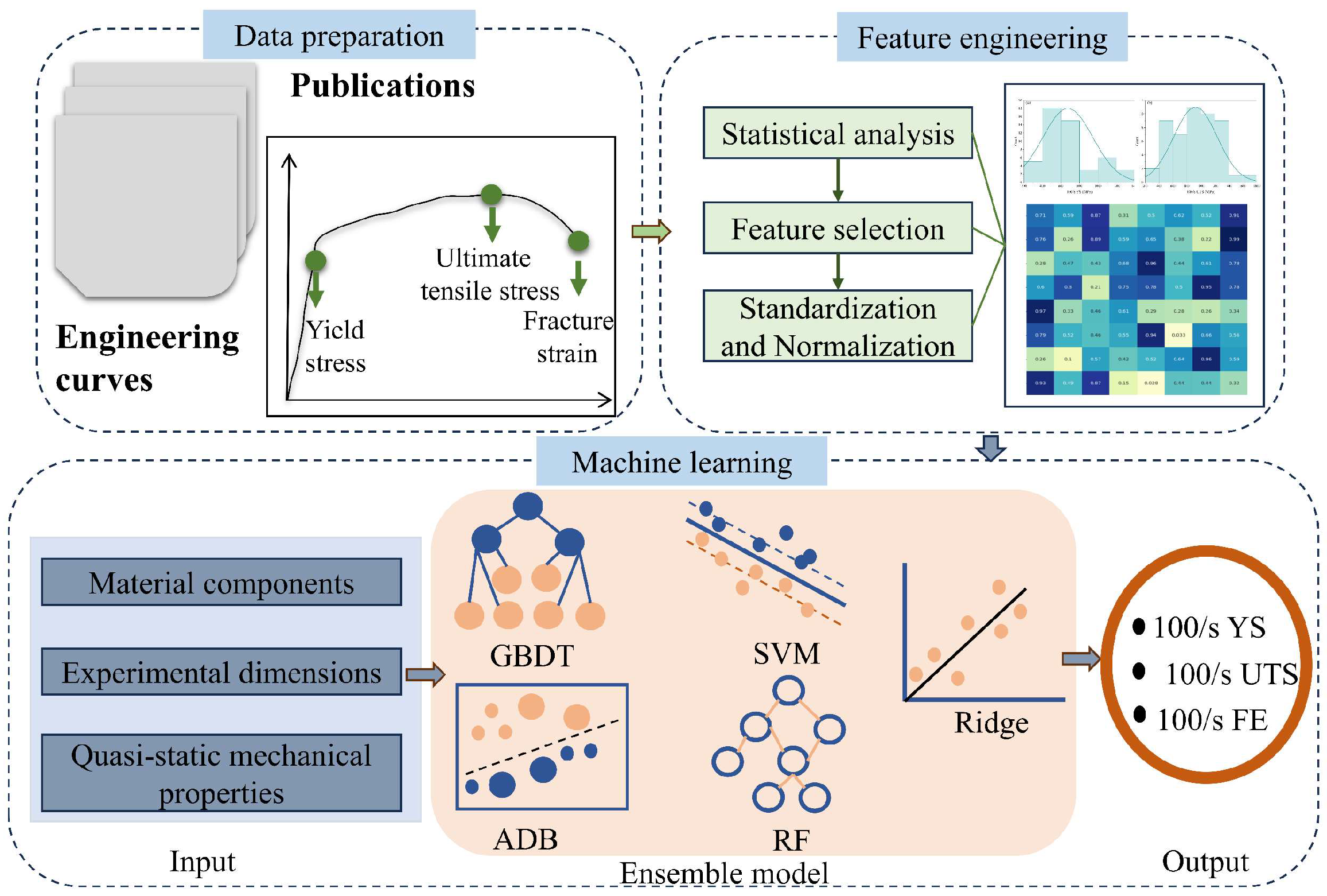
2. Methods
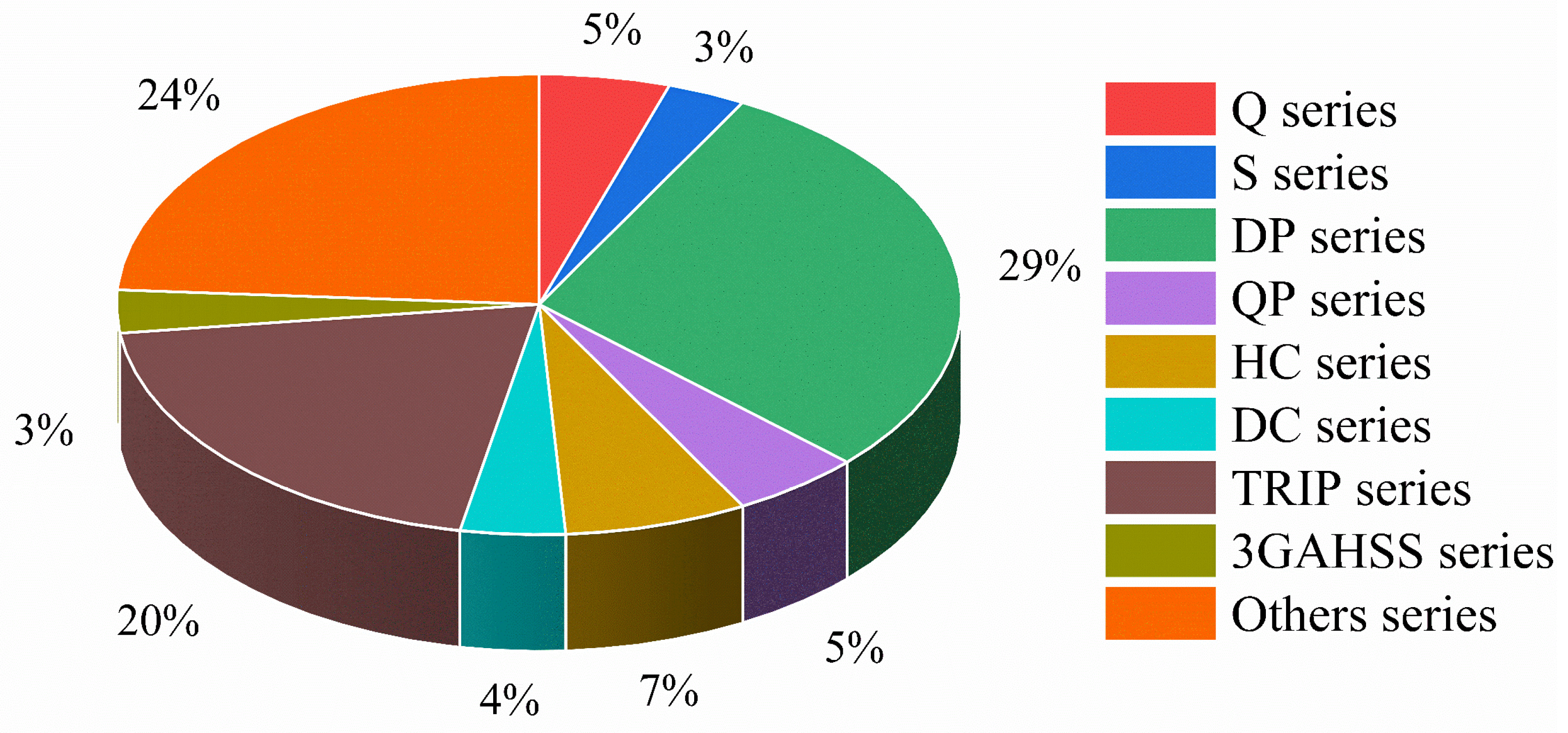
2.1. Data Collection and Preprocessing
2.2. Machine Learning Model Building and Performance Evaluation
2.3. Shapley Additive Explanation (SHAP)
3. Results and Discussion
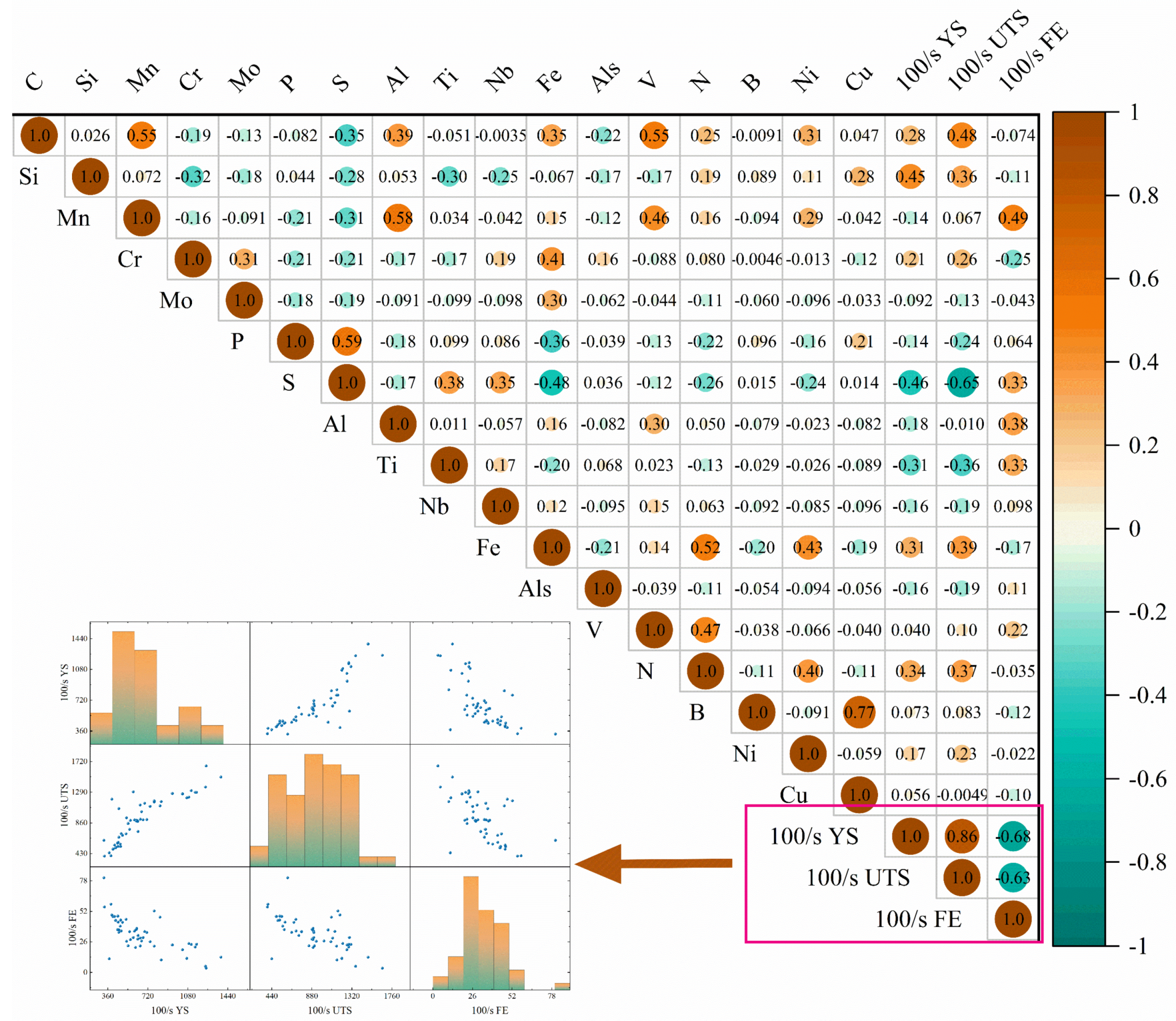
3.1. Feature Selection Results
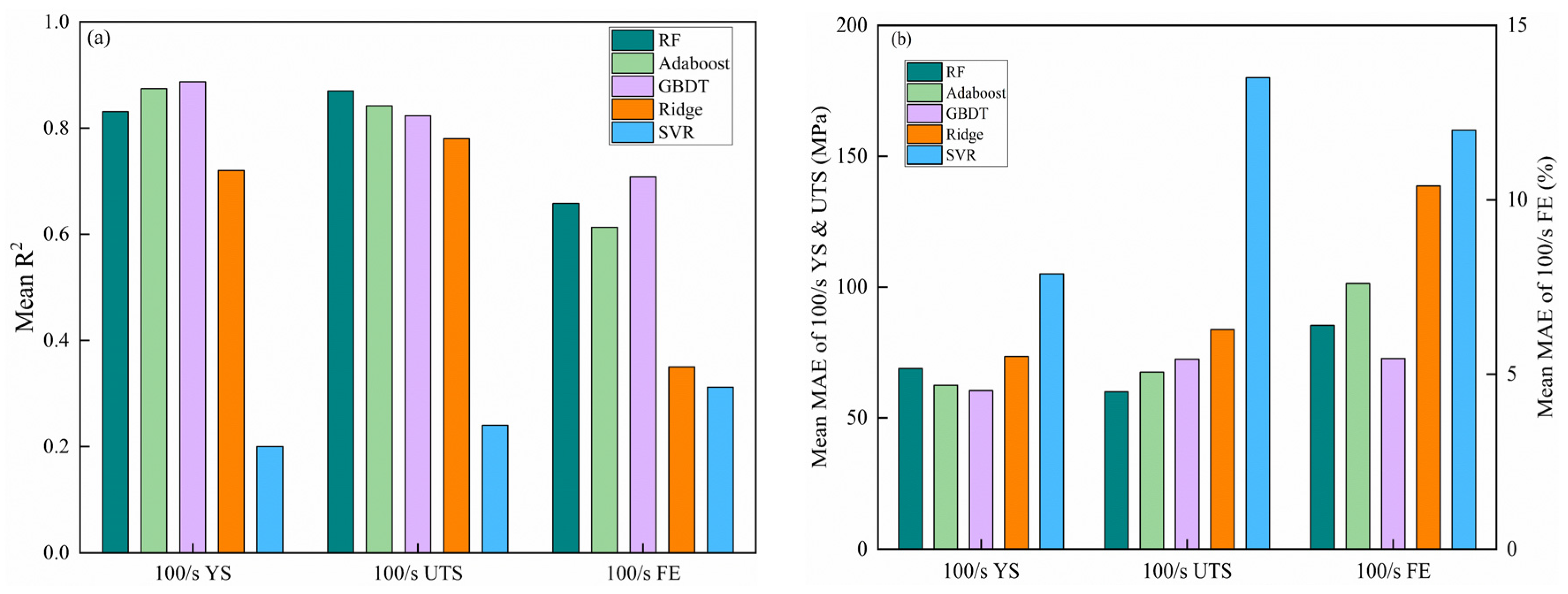
3.2. Model-Predicted Performance Results
3.2.1. Single Model
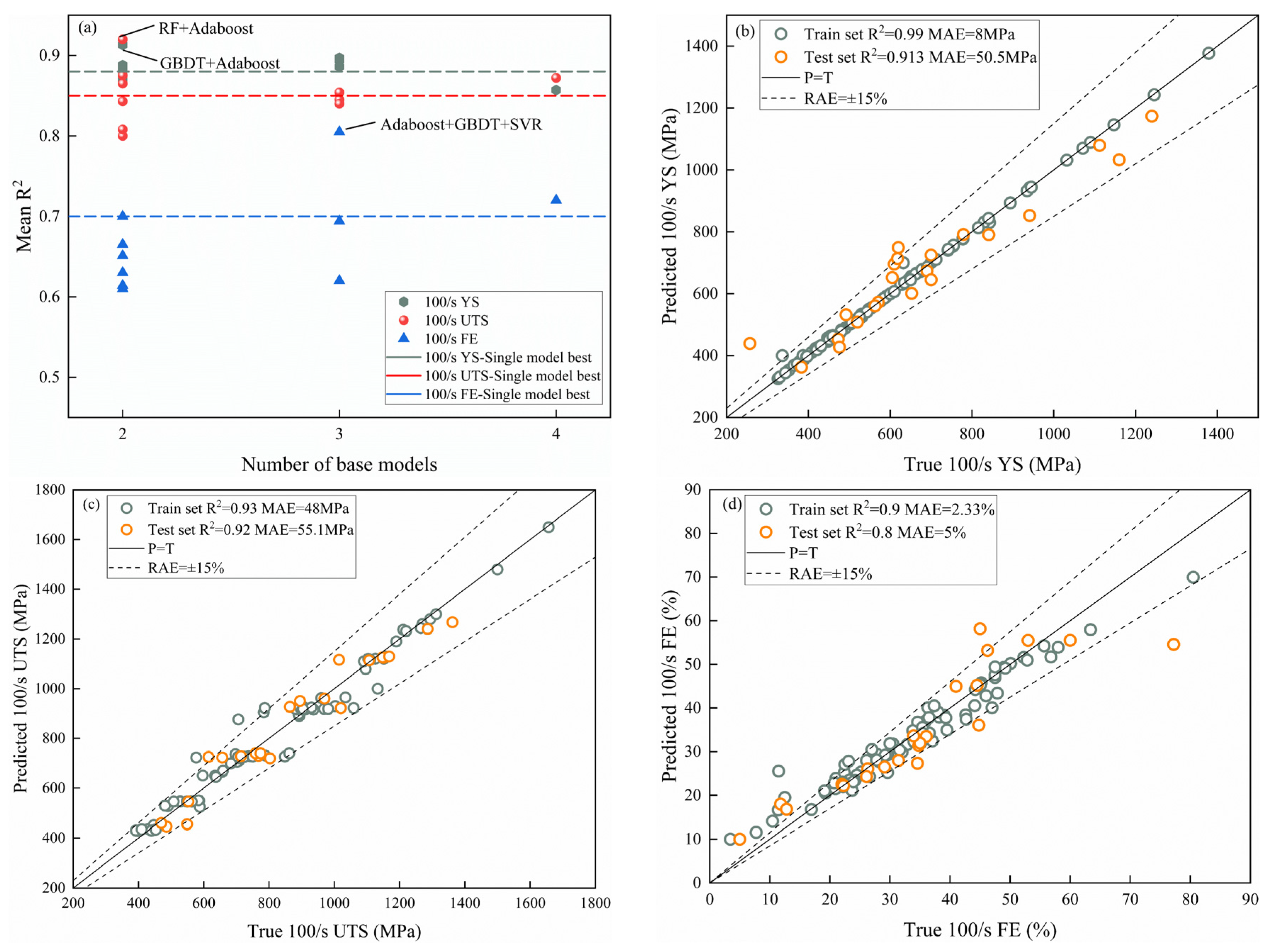
3.2.2. Ensemble Model
3.3. SHAP-Based Analysis of Feature Importance
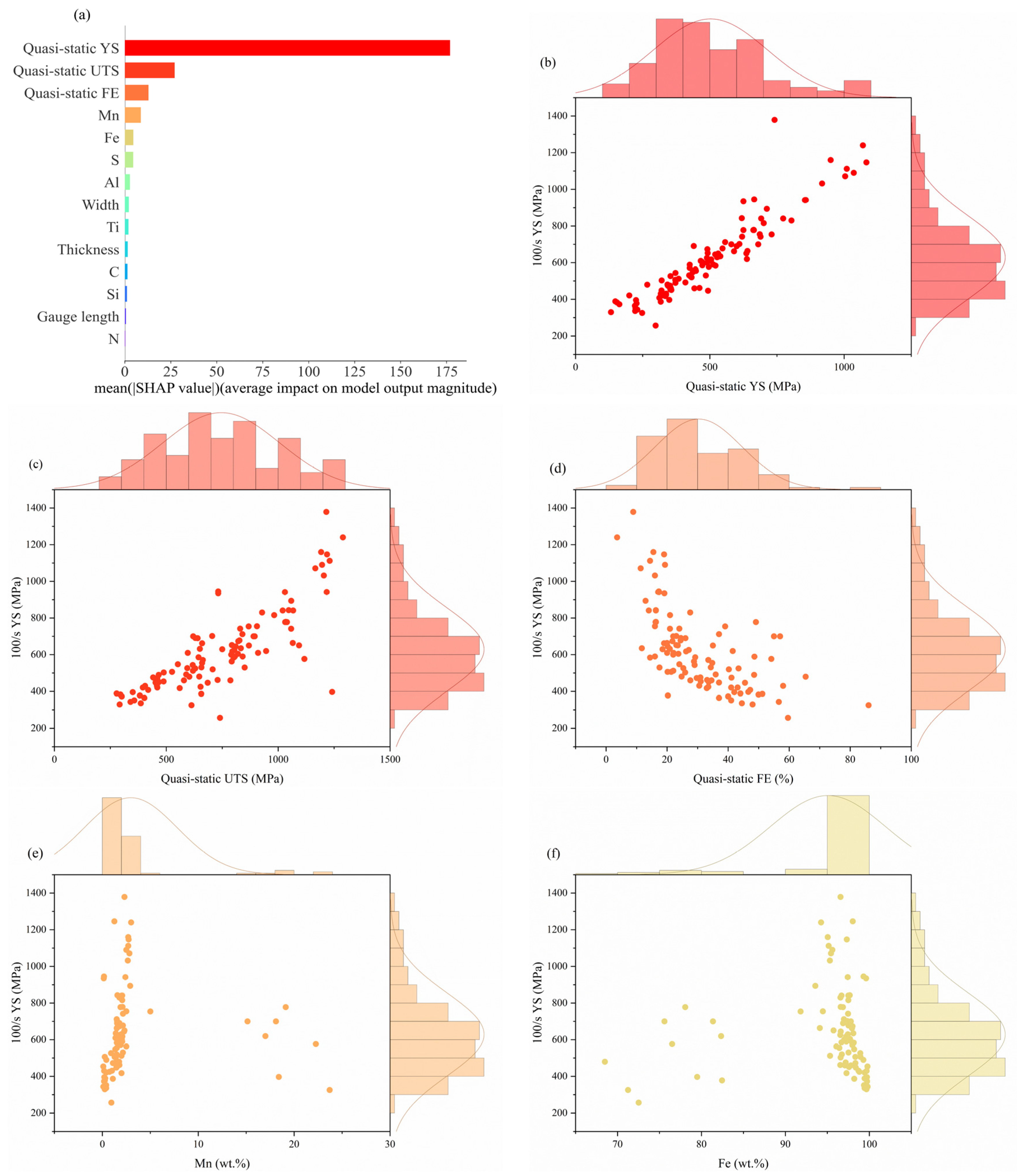
3.3.1. For 100/s YS
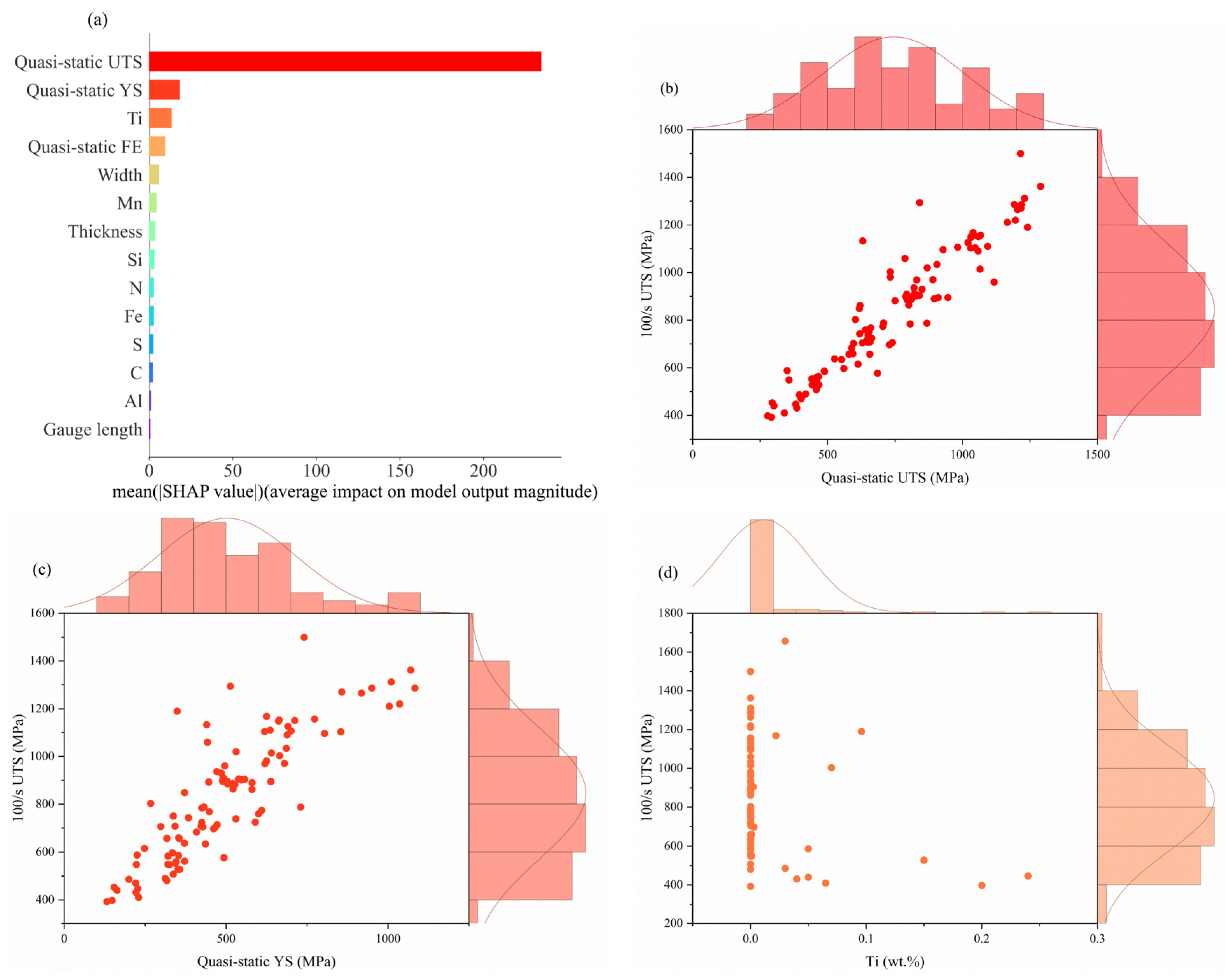
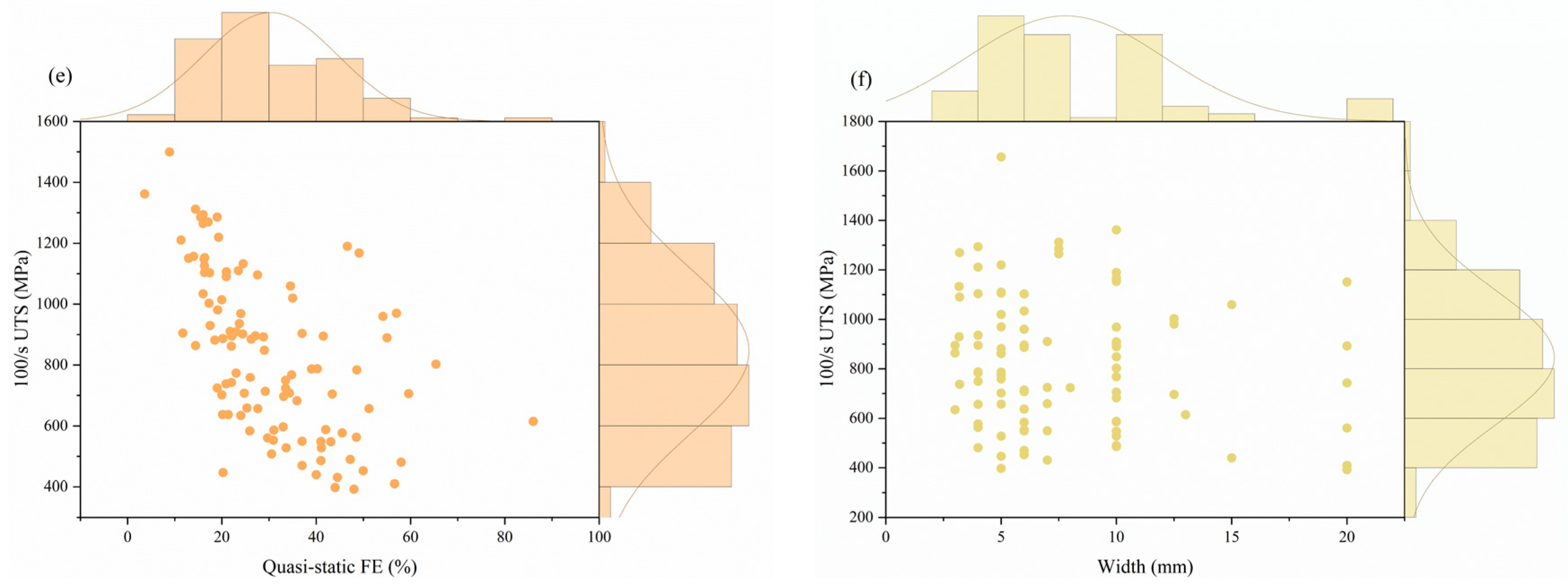
3.3.2. For 100/s UTS
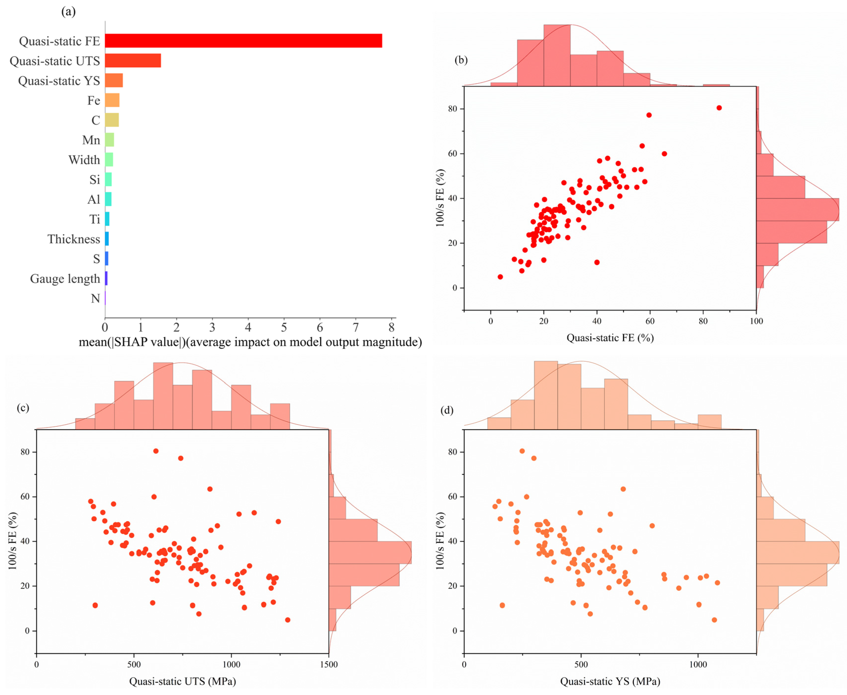
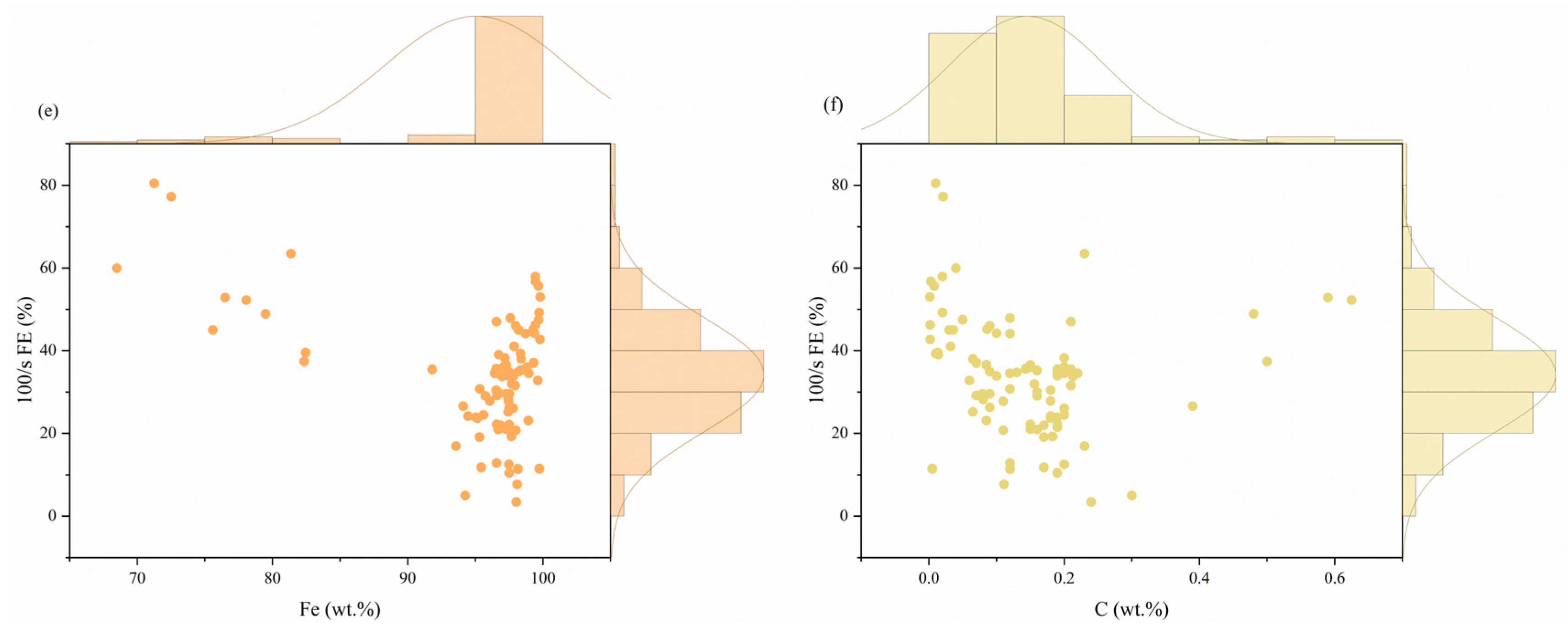
3.3.3. For 100/s FE
4. Conclusions
- A dataset was constructed by collecting the high-speed tensile experimental data of 65 kinds of automotive steels. Based on five ML algorithms, including Ridge regression, SVR, RF, GBDT, and Adaboost, the composition, sample size, quasi-static mechanical properties, and mechanical properties at 100/s were established. Compared with these models, GBDT is considered to be the best model for predicting 100/s YS and 100/FE, and RF is the best model for predicting 100/s UTS.
- Based on the idea of stacking integration, a super learner is built based on the ML model mentioned above to further improve the model prediction performance. The results show that the integrated model has better predictive performance and generalization performance, and the R2 scores are as high as 0.913, 0.92, and 0.8, with lower MAE on the test sets of 100/s YS, 100/s UTS, and 100/s FE.
- Based on a SHAP analysis, the main characteristics that significantly affect the tensile properties at intermediate strain rates are revealed, in which the quasi-static mechanical properties dominate. Secondly, Mn, Ti, and C have significant effects on the prediction of YS, UTS, and FE, respectively.
Supplementary Materials
Author Contributions
Funding
Data Availability Statement
Conflicts of Interest
References
- Tang, Z.Y.; Huang, J.N.; Ding, H.; Cai, Z.; Misra, R. On the dynamic behavior and relationship to mechanical properties of cold-rolled Fe-0.2 C-15Mn-3Al steel at intermediate strain rate. Mater. Sci. Eng. A 2019, 742, 423–431. [Google Scholar] [CrossRef]
- Yang, X.; Yang, H.; Lai, Z.; Zhang, S. Dynamic tensile behavior of S690 high-strength structural steel at intermediate strain rates. J. Constr. Steel Res. 2020, 168, 105961. [Google Scholar] [CrossRef]
- Li, W.; Chen, H. Tensile performance of normal and high-strength structural steels at high strain rates. Thin-Walled Struct. 2023, 184, 110457. [Google Scholar] [CrossRef]
- Cui, J.; Wang, Q.; Dong, D.; Jiang, H.; Zhang, X.; Li, G. A study on the constitutive equation of HC420LA steel subjected to high strain rates. J. Mater. Res. 2019, 34, 1034–1042. [Google Scholar] [CrossRef]
- Rajendra, P.; Girisha, A.; Naidu, T.G. Advancement of machine learning in materials science. Mater. Today Proc. 2022, 62, 5503–5507. [Google Scholar] [CrossRef]
- Golmohammadi, M.; Aryanpour, M. Analysis and evaluation of machine learning applications in materials design and discovery. Mater. Today Commun. 2023, 35, 105494. [Google Scholar] [CrossRef]
- Bhat, N.; Barnard, A.S.; Birbilis, N. Improving the prediction of mechanical properties of aluminium alloy using data-driven class-based regression. Comput. Mater. Sci. 2023, 228, 112270. [Google Scholar] [CrossRef]
- Gong, H.; Fan, Q.; Xie, W.; Zhang, H.; Yang, L.; Xu, S.; Cheng, X. Mining the relationship between the dynamic compression performance and basic mechanical properties of Ti20C based on machine learning methods. Mater. Des. 2023, 226, 111633. [Google Scholar] [CrossRef]
- Li, S.-G.; Chen, Q.-R.; Huang, L.; Chen, M.; Wei, C.-D.; Yue, Z.-J.; Liu, R.-X.; Tong, C.; Liu, Q. Data-driven approach to predict the fatigue properties of ferrous metal materials using the cGAN and machine-learning algorithms. Adv. Manuf. 2024, 12, 447–464. [Google Scholar] [CrossRef]
- Wang, S.; Li, J.; Zuo, X.; Chen, N.; Rong, Y. An optimized machine-learning model for mechanical properties prediction and domain knowledge clarification in quenched and tempered steels. J. Mater. Res. Technol. 2023, 24, 3352–3362. [Google Scholar] [CrossRef]
- Zhu, Y.; Yang, H.; Zhang, S. Dynamic mechanical behavior and constitutive models of S890 high-strength steel at intermediate and high strain rates. J. Mater. Eng. Perform. 2020, 29, 6727–6739. [Google Scholar] [CrossRef]
- Wang, H.; Huo, J.; Liu, Y. Experimental study on dynamic tensile performance of Q345 structural steel considering thickness differences. In Structures; Elsevier: Amsterdam, The Netherlands, 2023; pp. 891–910. [Google Scholar]
- Chen, J.; Shu, W.; Li, J. Constitutive model of Q345 steel at different intermediate strain rates. Int. J. Steel Struct. 2017, 17, 127–137. [Google Scholar] [CrossRef]
- Yu, P.; Zhang, J.; Zhang, C.; Zhao, J. Strain-rate-dependent constitutive and damage models for a low-yielding-strength steel under dynamic loadings. J. Mech. Sci. Technol. 2021, 35, 4405–4417. [Google Scholar] [CrossRef]
- Alturk, R.; Hector, L.G.; Matthew Enloe, C.; Abu-Farha, F.; Brown, T.W. Strain rate effect on tensile flow behavior and anisotropy of a medium-manganese TRIP steel. JOM 2018, 70, 894–905. [Google Scholar] [CrossRef]
- Madivala, M.; Bleck, W. Strain rate dependent mechanical properties of TWIP steel. JOM 2019, 71, 1291–1302. [Google Scholar] [CrossRef]
- Benesty, J.; Chen, J.; Huang, Y. On the importance of the Pearson correlation coefficient in noise reduction. IEEE Trans. Audio Speech Lang. Process. 2008, 16, 757–765. [Google Scholar] [CrossRef]
- Ruppert, D. The Elements of Statistical Learning: Data Mining, Inference, and Prediction; Taylor & Francis: Abingdon, UK, 2004. [Google Scholar]
- Laan, M.J.v.d.; Polley, E.C.; Hubbard, A.E. Super Learner. Stat. Appl. Genet. Mol. Biol. 2007, 6, 23. [Google Scholar] [CrossRef]
- Lundberg, S.M.; Lee, S.-I. A unified approach to interpreting model predictions. Adv. Neural Inf. Process. Syst. 2017, 30, 4765–4774. [Google Scholar]
- Mangalathu, S.; Hwang, S.-H.; Jeon, J.-S. Failure mode and effects analysis of RC members based on machine-learning-based SHapley Additive exPlanations (SHAP) approach. Eng. Struct. 2020, 219, 110927. [Google Scholar] [CrossRef]
- Hou, H.; Wang, J.; Ye, L.; Zhu, S.; Wang, L.; Guan, S. Prediction of mechanical properties of biomedical magnesium alloys based on ensemble machine learning. Mater. Lett. 2023, 348, 134605. [Google Scholar] [CrossRef]
- Suh, J.S.; Kim, Y.M.; Yim, C.D.; Suh, B.-C.; Bae, J.H.; Lee, H.W. Interpretable machine learning-based analysis of mechanical properties of extruded Mg-Al-Zn-Mn-Ca-Y alloys. J. Alloys Compd. 2023, 968, 172007. [Google Scholar] [CrossRef]
- Mukhopadhyay, A.; Das, S.; Mukhopadhyay, G. Effect of Pre-Strain and Strain Rate on Deformation and Fracture Behavior of Automotive Grade Interstitial Free Steel Sheets. J. Mater. Eng. Perform. 2024, 1–17. [Google Scholar] [CrossRef]

| Features | Min | Max | Mean | SD | |
|---|---|---|---|---|---|
| Input features | C (wt.%) | 0.0014 | 0.625 | 0.1453 | 0.11719 |
| Si (wt.%) | 0 | 3.15 | 0.53 | 0.66627 | |
| Mn (wt.%) | 0.1 | 23.7 | 2.96183 | 4.87571 | |
| Cr (wt.%) | 0 | 18.31 | 0.64016 | 3.12958 | |
| Mo (wt.%) | 0 | 2.11 | 0.03593 | 0.23381 | |
| P (wt.%) | 0 | 0.25 | 0.0207 | 0.03024 | |
| S (wt.%) | 0 | 0.5 | 0.01248 | 0.05293 | |
| Al (wt.%) | 0 | 3.5 | 0.33424 | 0.82122 | |
| Ti (wt.%) | 0 | 0.24 | 0.01182 | 0.03915 | |
| Nb (wt.%) | 0 | 0.12 | 0.00778 | 0.02073 | |
| Fe (wt.%) | 68.493 | 99.805 | 95.071 | 6.8766 | |
| Als (wt.%) | 0 | 0.04 | 0.00198 | 0.00822 | |
| V (wt.%) | 0 | 0.487 | 0.01085 | 0.06213 | |
| N (wt.%) | 0 | 0.019 | 0.0009 | 0.00277 | |
| B (wt.%) | 0 | 3.15 | 0.53024 | 0.66627 | |
| Ni (wt.%) | 0 | 10.72 | 0.21765 | 1.39556 | |
| Cu (wt.%) | 0 | 0.4 | 0.01674 | 0.0672 | |
| Gauge length (mm) | 5 | 50 | 18.077 | 8.673 | |
| Width (mm) | 3 | 20 | 7.79432 | 4.283 | |
| Thickness (mm) | 0.6 | 6 | 1.4681 | 0.702 | |
| Quasi-static YS (MPa) | 132 | 1083 | 502.47 | 212.334 | |
| Quasi-static UTS (MPa) | 278 | 1289 | 745.52 | 261.5 | |
| Quasi-static FE (%) | 3.6 | 86 | 30.32 | 14.26 | |
| Output features | 100/s YS (MPa) | 257 | 1379 | 628.76 | 226.648 |
| 100/s UTS (MPa) | 392.47 | 1656.91 | 845.627 | 272.561 | |
| 100/s FE (%) | 3.437 | 80.5 | 34.193 | 13.91 |
| Base Model | R2 | MAE | ||||
|---|---|---|---|---|---|---|
| 100/s YS | 100/s UTS | 100/s FE | 100/s YS (MPa) | 100/s UTS (MPa) | 100/s FE (%) | |
| RF-Adaboost | 0.913 | 0.875 | 0.7 | 50.5 | 63 | 5.8 |
| RF-GBDT | 0.888 | 0.843 | 0.614 | 58 | 69.7 | 7.8 |
| RF-SVR | 0.87 | 0.865 | 0.665 | 60 | 64 | 6.98 |
| Adaboost-GBDT | 0.875 | 0.92 | 0.651 | 58.9 | 55.1 | 7.3 |
| Adaboost-SVR | 0.884 | 0.8 | 0.63 | 58.5 | 75.8 | 7.4 |
| GBDT-SVR | 0.868 | 0.808 | 0.61 | 62 | 75 | 6.2 |
| RF-Adaboost-GBDT | 0.886 | 0.854 | 0.694 | 60.4 | 68 | 6 |
| RF-Adaboost-SVR | 0.897 | 0.845 | 0.62 | 54 | 70 | 6.1 |
| Adaboost-GBDT-SVR | 0.894 | 0.84 | 0.8 | 54.8 | 69 | 5 |
| Adaboost-GBDT-SVR-RF | 0.857 | 0.872 | 0.557 | 63 | 62 | 6.5 |
Disclaimer/Publisher’s Note: The statements, opinions and data contained in all publications are solely those of the individual author(s) and contributor(s) and not of MDPI and/or the editor(s). MDPI and/or the editor(s) disclaim responsibility for any injury to people or property resulting from any ideas, methods, instructions or products referred to in the content. |
© 2025 by the authors. Published by MDPI on behalf of the World Electric Vehicle Association. Licensee MDPI, Basel, Switzerland. This article is an open access article distributed under the terms and conditions of the Creative Commons Attribution (CC BY) license (https://creativecommons.org/licenses/by/4.0/).
Share and Cite
Wang, H.; Lv, F.; Zhan, Z.; Zhao, H.; Li, J.; Yang, K. Predicting the Tensile Properties of Automotive Steels at Intermediate Strain Rates via Interpretable Ensemble Machine Learning. World Electr. Veh. J. 2025, 16, 123. https://doi.org/10.3390/wevj16030123
Wang H, Lv F, Zhan Z, Zhao H, Li J, Yang K. Predicting the Tensile Properties of Automotive Steels at Intermediate Strain Rates via Interpretable Ensemble Machine Learning. World Electric Vehicle Journal. 2025; 16(3):123. https://doi.org/10.3390/wevj16030123
Chicago/Turabian StyleWang, Houchao, Fengyao Lv, Zhenfei Zhan, Hailong Zhao, Jie Li, and Kangte Yang. 2025. "Predicting the Tensile Properties of Automotive Steels at Intermediate Strain Rates via Interpretable Ensemble Machine Learning" World Electric Vehicle Journal 16, no. 3: 123. https://doi.org/10.3390/wevj16030123
APA StyleWang, H., Lv, F., Zhan, Z., Zhao, H., Li, J., & Yang, K. (2025). Predicting the Tensile Properties of Automotive Steels at Intermediate Strain Rates via Interpretable Ensemble Machine Learning. World Electric Vehicle Journal, 16(3), 123. https://doi.org/10.3390/wevj16030123