Enhancing Thermal Comfort and Efficiency in Fuel Cell Trucks: A Predictive Control Approach for Cabin Heating

Abstract

Fuel cell trucks are a promising solution to reduce the disproportionately high greenhouse gas emissions of heavy-duty long-haul transportation. However, unlike conventional diesel vehicles, they lack combustion engine waste heat for cabin heating. As a result, electric heaters are often employed, which increase auxiliary energy consumption and reduce driving range. To address this challenge, advanced control strategies are needed to improve heating efficiency while maintaining passenger comfort. This study proposes and validates a methodology for implementing Model Predictive Control (MPC) in the cabin heating system of a fuel cell truck. Vehicle experiments were conducted to characterize dynamic heating behavior, passenger comfort indices, and to provide validation data for the mathematical models. Based on these models, an MPC strategy was developed in a Model-in-the-Loop simulation environment. The proposed approach achieves energy savings of up to 8.1% compared with conventional control using purely electric heating, and up to 21.7% when cabin heating is coupled with the medium-temperature cooling circuit. At the same time, passenger comfort is maintained within the desired range (PMV within ±0.5 under typical winter conditions). The results demonstrate the potential of MPC to enhance the energy efficiency of fuel cell trucks. The methodology presented provides a validated foundation for the further development of predictive thermal management strategies in heavy-duty zero-emission vehicles.

1. Introduction

Looking at the automotive industry today, one can observe a fundamental transformation taking place. The electrification of vehicles is progressing rapidly, particularly in the passenger car segment. Although commercial vehicles (CVs) offer considerable potential for reducing greenhouse gas emissions, their electrification is advancing much more slowly.

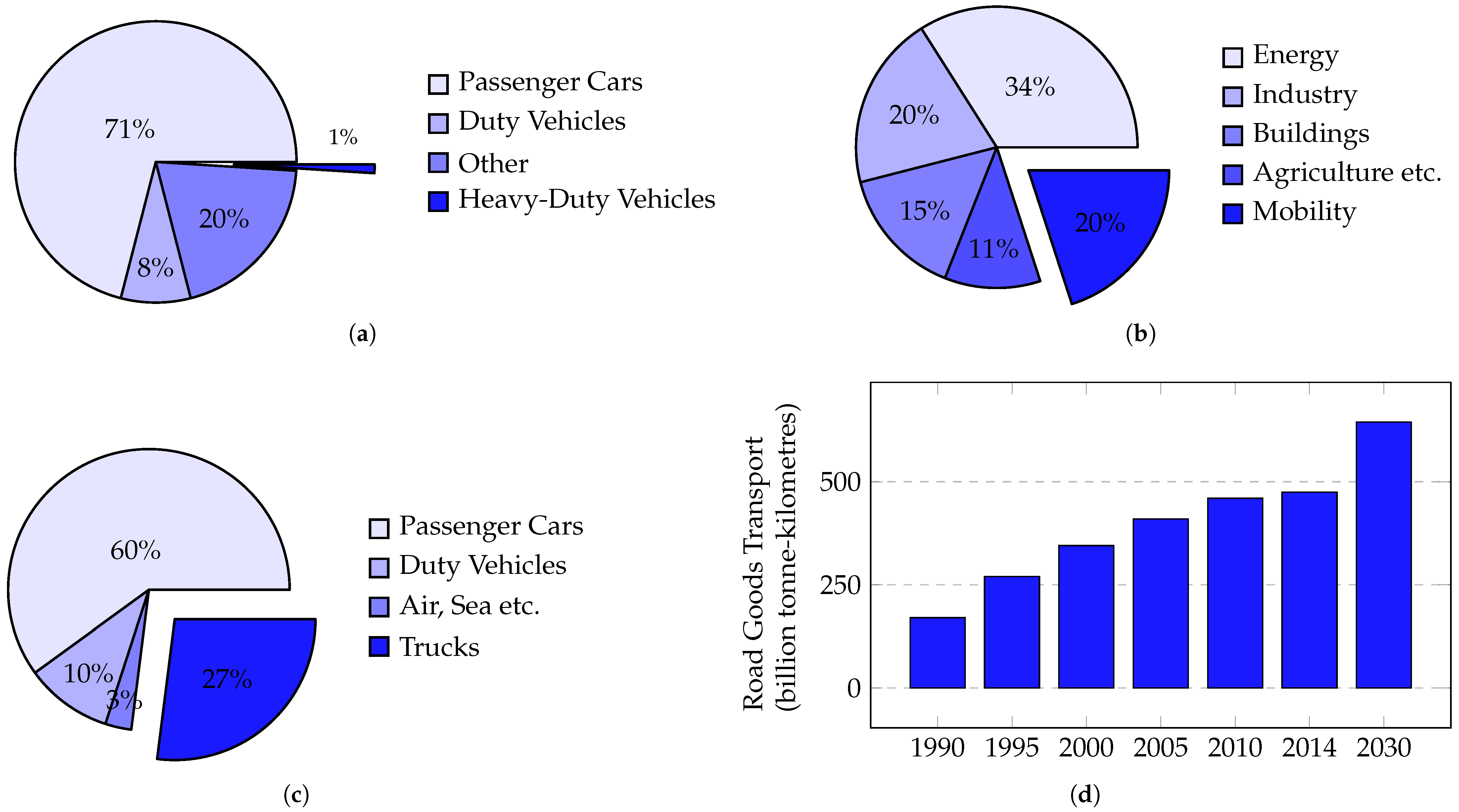
Figure 1 highlights the motivation to electrify heavy-duty trucks. When examining the vehicle distribution in Germany in 2022, shown in Figure 1a, it becomes clear that heavy-duty vehicles account for only about 1% of the total vehicle fleet [1]. However, as illustrated in Figure 1c, they are responsible for approximately 27% of total CO₂ emissions in the mobility sector [2]. Considering that the mobility sector contributes around 20% of total CO₂ emissions in Germany (Figure 1b) [3], the potential for reducing greenhouse gas emissions from heavy-duty trucks is substantial. Furthermore, given the projected increase in road freight transport from 2014 to 2030 (Figure 1d) [4], the electrification of this vehicle class becomes even more crucial to achieving climate goals.

The significant share of total emissions from heavy-duty long-haul trucks is primarily due to their high weight and high mileage. Replacing the traditional diesel drivetrain with an electrified one therefore offers considerable potential for reducing overall greenhouse gas emissions. However, vehicles in this weight class are still predominantly diesel-powered. In 2021, only about 1% of new registrations in the EU met the standard for zero-emission vehicles [5]. This is expected to change in the foreseeable future, as electrification is increasingly emerging in this vehicle segment. Most OEMs (Original Equipment Manufacturers) now offer battery-electric trucks (e.g., DAF, Scania, Daimler, MAN) and some even fuel cell electric trucks (e.g., Hyundai).

The research presented in this paper was conducted within the project SeLv, funded by the Federal Ministry of Transport (BMV). The project’s aim is to develop a modular electric powertrain for long-haul heavy-duty trucks. Its scope includes converting three 40-tonne conventional diesel trucks to electric drivetrains with fuel cells as range extenders [6].

A number of approaches and technologies are currently being considered to enable zero-emission operation of heavy-duty trucks. The most commonly discussed powertrain technologies are battery-electric, fuel cell electric, and catenary electric trucks [7]. Overhead line (catenary) electric trucks pose challenges due to the expensive motorway infrastructure they require [7]. Battery-electric trucks are locally emission-free but face the challenge of excessive drivetrain weight, which limits their suitability for the long ranges required in this vehicle class. Even with expected advancements in battery energy density, a battery-electric heavy-duty truck would still be significantly heavier than both diesel and fuel cell alternatives—by approximately $900\mathrm{kg}$ and $2300\mathrm{kg}$ for $800\mathrm{km}$ and $1200\mathrm{km}$ ranges, respectively [8].

Fuel cell electric trucks, in contrast, can achieve the required long ranges with an acceptable drivetrain weight while producing zero tailpipe emissions. Moreover, the hydrogen used in fuel cells can be produced from renewable energy via water electrolysis, offering a pathway to substantial CO₂ reductions. Complementary approaches, such as solid oxide electrolysis cells (SOECs), enable the conversion of renewable electricity and captured CO₂ into synthetic fuels for power-to-X applications, thereby supporting the broader decarbonization of the transport sector [9].

However, the adoption of such alternative powertrains introduces challenges that are not present in conventional systems. One of the main challenges for fuel cell trucks is thermal management, which offers significant potential for optimization due to its complexity and high energy demand. This has been highlighted by both expert interviews in a study comparing hydrogen combustion engines and fuel cells for trucks [10] and by the findings of the SeLv project [6]. Simulation results from this project suggest that thermal management can account for approximately 14% of total vehicle energy consumption over a driving cycle at cold ambient temperatures (−20 °C) and 12% under hot conditions (40 °C).

The cabin heating system is vital for ensuring thermal comfort, particularly in colder climates. Maintaining cabin comfort is crucial for driver well-being, especially in long-haul trucks where drivers spend extended periods inside. Creating a pleasant cabin environment affects not only comfort but also safety. Human thermal stress is described by the internationally recognized thermal comfort index PMV (Predicted Mean Vote). At $\mathrm{PMV}=0$, approximately 95% of respondents feel thermally comfortable, while at $\mathrm{PMV}=1$, this drops to around 75%. A change from PMV 0 to PMV 1 increases the probability of traffic accidents in urban areas by 11%. At $\mathrm{PMV}=2$, the increase is twice as high, that is, 22%. Outside urban areas, the effect is less pronounced but still relevant: PMV values of 1, 2, and 3 lead to increases in accident frequency of 6%, 13%, and 18%, respectively [11].

Efforts to improve thermal comfort often result in increased energy consumption, as maintaining consistent temperatures becomes more demanding under fluctuating external conditions. In extreme weather scenarios, the heating, ventilation, and air conditioning (HVAC) system can account for up to 50% of total energy usage in a battery electric vehicle (BEV) [12]. This substantial energy demand directly impacts vehicle range, highlighting a critical trade-off between energy efficiency and passenger comfort. Consequently, effective management and control of the heating system are essential to balance these competing priorities.

Traditional controllers, such as Proportional-Integral-Derivative (PID) [13] and On/Off controllers [14], have been widely used in HVAC systems. However, they often struggle to handle the nonlinearities inherent in vehicle HVAC systems and the continuously changing external disturbances [15]. Similarly, in fuel cell vehicles, conventional control strategies may not adequately address challenges such as high-voltage-induced degradation and rapid transient responses [16]. This has motivated the development of advanced control schemes, including fuzzy-LQG and hybrid controllers, to improve performance and durability. Model Predictive Control (MPC) offers another promising solution, as it can predict system behavior, handle constraints, and optimize control actions under varying operating conditions [17,18]. Unlike conventional rule-based or PID controllers, MPC includes a customizable cost function that enables tailored optimization strategies. This paper investigates the potential of MPC to improve the efficiency of the heating system in heavy-duty electrified trucks by anticipating future thermal demands and optimizing the trade-off between energy consumption and cabin comfort.

The main contributions of this paper are threefold. First, one of the first applications of MPC to the heating system of heavy-duty fuel cell trucks is presented, addressing the unique requirements of long-haul commercial vehicles. Second, the energy efficiency improvements and cabin comfort benefits of the proposed approach are quantified in comparison to conventional controllers, based on a validated simulation model. Third, the coupling of the cabin heating loop with the medium-temperature cooling circuit is analyzed, demonstrating how MPC can effectively manage complex multi-input, multi-output subsystem interactions.

2. Fundamentals of Model Predictive Control

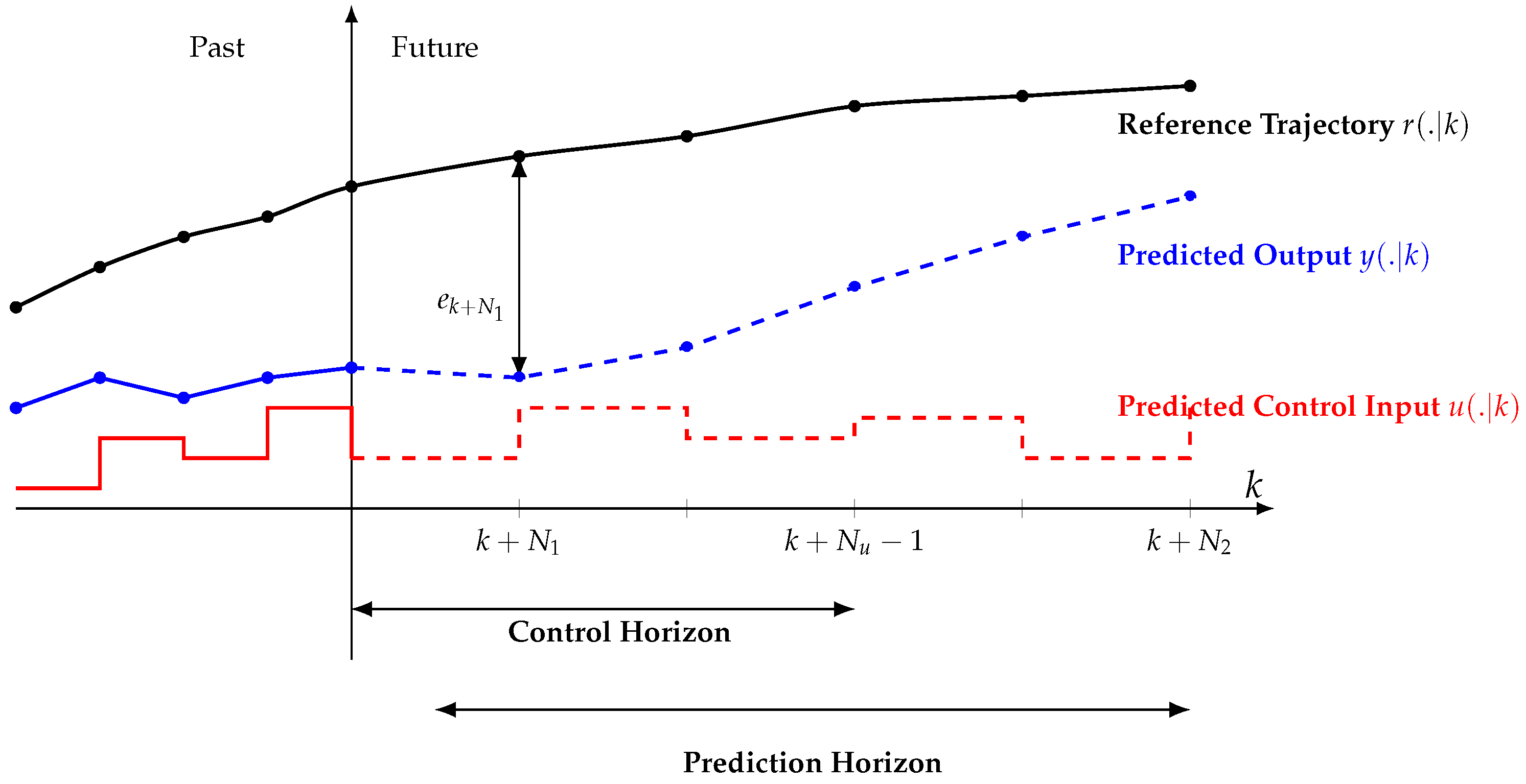
Model predictive control is an advanced control approach that relies on a system model to predict future states and compute a control vector that minimises a cost function over a defined prediction horizon while accounting for disturbances and constraints. At each time step, only the first element of the computed control vector is applied to the system input, and the remaining elements are discarded. This process is then repeated at the subsequent time instant. The cost function can encompass factors such as tracking errors, actuator effort, energy cost, power consumption, or a combination of these elements. Constraints may be imposed on the rate and range limits of the actuators and the manipulated and controlled variables [17]. Figure 2 shows the basic principle of MPC [19].

Most control tasks in thermal management can be formulated as reference tracking problems, where the objective is to ensure the system follows a desired trajectory or operating behavior. A common distinction is made between linear and nonlinear model predictive control (MPC). Since the system model in linear MPC (LMPC) is restricted to being linear or linearized, nonlinear approaches are generally more suitable for real-world problems, as they offer improved control performance [20].

Through physical modeling, one typically obtains continuous-time models of nonlinear systems. These continuous-time nonlinear models serve as the basis for optimization-based control algorithms, resulting in what is known as an Optimal Control Problem (OCP). In an OCP, the controller computes an optimal input trajectory by minimizing a cost function, such as the following example cost function $J_{OCP}$ [20]:

$$J_{OCP}(x\left(t\right),u\left(t\right))=l_f\left(x\left(t_f\right)\right)+{\int }_{t_0}^{t_f}{l}_s(x\left(t\right),u\left(t\right))dt$$

(1)

This standard optimization problem can be defined as follows:

$$\begin{array}{cc}\hfill \underset{x\left(t\right),u\left(t\right)}{min}& J_{OCP}(x\left(t\right),u\left(t\right))\hfill \end{array}$$

(2)

$$\begin{array}{cc}\hfill \mathrm{s}.\mathrm{t}.& \dot{x}=f(x\left(t\right),u\left(t\right),t),\forall t\in [t_0,t_f]\hfill \end{array}$$

(3)

$$\begin{array}{cc}\hfill & x\left(t_0\right)=x_0,\hfill \end{array}$$

(4)

$$\begin{array}{cc}\hfill & h\left(x\left(t_f\right)\right)=0,\hfill \end{array}$$

(5)

$$\begin{array}{cc}\hfill & g(x\left(t\right),u\left(t\right))\le 0,\forall t\in [t_0,t_f]\hfill \end{array}$$

(6)

where:

• $x\left(t\right)\in {\mathbb{R}}^n$ is the system state vector at time t
• $u\left(t\right)\in {\mathbb{R}}^m$ is the control input vector at time t
• $f\left(x\right(t),u(t),t)$ is the system dynamics function, defining the time evolution of the states
• $x_0$ is the initial condition of the state, i.e., $x\left(t_0\right)=x_0$
• $l_s(x\left(t\right),u\left(t\right))$ is the stage cost function, representing running costs over time
• $l_f\left(x\left(t_f\right)\right)$ is the terminal cost function, representing costs at the final time
• $h\left(x\left(t_f\right)\right)=0$ are terminal equality constraints on the state
• $g\left(x\right(t),u(t\left)\right)\le 0$ are path inequality constraints on the state and input.

Equation (3) subjects the cost function $J_{OCP}$ to system dynamics. Equation (4) describes the initial state of the system at $t=t_0$, while Equations (5) and (6) define equality constraints on the final states and path constraints, respectively [20].

3. Implementations of MPC in the Simulation

In this subsection, an MiL (Model-in-the-Loop) approach is presented. First, the modeling of the heating system is described. Next, the results of the model validation are shown, and finally, the implementation of the MPC in MiL is discussed.

3.1. Modeling of the Heating System

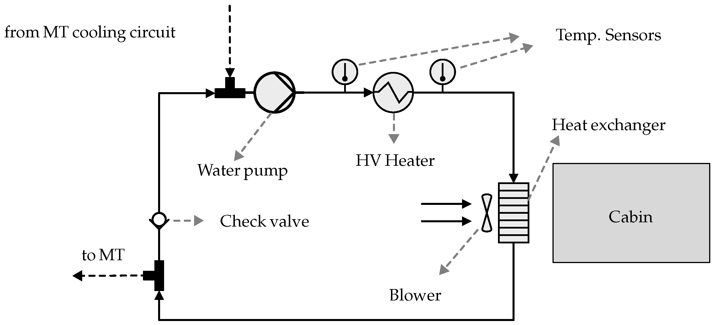
The structure of the cabin heating system in the SeLv truck is shown in Figure 3. The heating system consists of a water pump, a high-voltage heater, and a heat exchanger. The heat exchanger is integrated into a standard HVAC unit in the vehicle cabin. The HVAC unit includes a heater core (heat exchanger for heating), an evaporator for air conditioning, air-guiding flaps, and a blower that draws in ambient or recirculated air and forces it through the heat exchangers.

The working fluid, hereafter referred to as the coolant, is a mixture of 50% water and 50% ethylene glycol. The heater is equipped with sensors that measure the inlet and outlet coolant temperatures. The dashed lines and T-connectors indicate the possibility of coupling the heating circuit with the medium-temperature (MT) cooling circuit, enabling the use of waste heat for cabin heating, as demonstrated in previous PEM research [21].

While the HVAC unit also provides air conditioning via the evaporator, this study focuses on heating mode. A detailed analysis of the cooling functionality, including its modeling and control, is beyond the scope of this paper and would require separate consideration due to its distinct physical dynamics and operating conditions.

Thermodynamic modeling of the heating system describes the thermal dynamics of the coolant circulating through the circuit and passing through the heater and cabin heat exchanger. First, a mathematical model comprising differential equations is developed and then implemented in MATLAB/Simulink R2024a [22]. Two Simulink blocks represent the lumped thermal masses of the heater and the heat exchanger. By applying the first law of thermodynamics, expressions for the coolant outlet temperatures of these components are obtained. To capture transient behavior, the thermal mass of the coolant is also included.

Table 1. Coolant system nomenclature.

Variable	Explanation
$T_{H\text{-}in/out}$	Coolant inlet/outlet temperature of the heater
$T_{HX\text{-}in/out}$	Coolant inlet/outlet temperature of the heat exchanger
$\dot{m}$	Coolant mass flow rate
$c_{p,w}$	Specific heat capacity of coolant

defines the nomenclature used to describe the heating system.

Equation (7) describes the transient behavior of the first portion of the coolant thermal mass, namely, the coolant volume in the system downstream of the heater. This transient formulation is necessary to capture the time-dependent temperature response during variations in heater power or coolant flow, which cannot be represented by a steady-state model. The resulting temperature is then used as the inlet condition for the heat exchanger.

$$m_H·c_{p,w}·{\displaystyle \frac{d{T}_{HX\text{-}in}}{dt}}=\dot{m}·c_{p,w}·(T_{H\text{-}out}-T_{HX\text{-}in})$$

(7)

where $m_H$ is the thermal mass of the coolant volume in the system downstream of the heater.

The volume of coolant in the system after the heat exchanger is considered as the second part of the coolant thermal mass. The corresponding heat balance equation is given in Equation (8), where the resulting temperature is used as the inlet temperature to the HV heater.

$$m_R·c_{p,w}·{\displaystyle \frac{d{T}_{H\text{-}in}}{dt}}=\dot{m}·c_{p,w}·(T_{HX\text{-}out}-T_{H\text{-}in})$$

(8)

Here, $m_R$ denotes the thermal mass of the coolant volume after the heat exchanger.

The coolant outlet temperature of the heater is determined from Equation (9), derived from a steady-state energy balance between the enthalpy change of the coolant and the input power of the heater.

$$T_{H\text{-}out}=T_{H\text{-}in}+{\displaystyle \frac{P_H}{\dot{m}·c_{p,w}}}$$

(9)

Here, $P_H$ denotes the input power of the heater.

The coolant temperature change in the heat exchanger is determined using Equation (10).

$$T_{HX\text{-}out}=T_{HX\text{-}in}+{\displaystyle \frac{-P_{E-NTU}}{\dot{m}·c_{p,w}}}$$

(10)

Here, $P_{E\text{-}NTU}$ represents the energy transferred from the coolant to the air, which will be modeled in the following section.

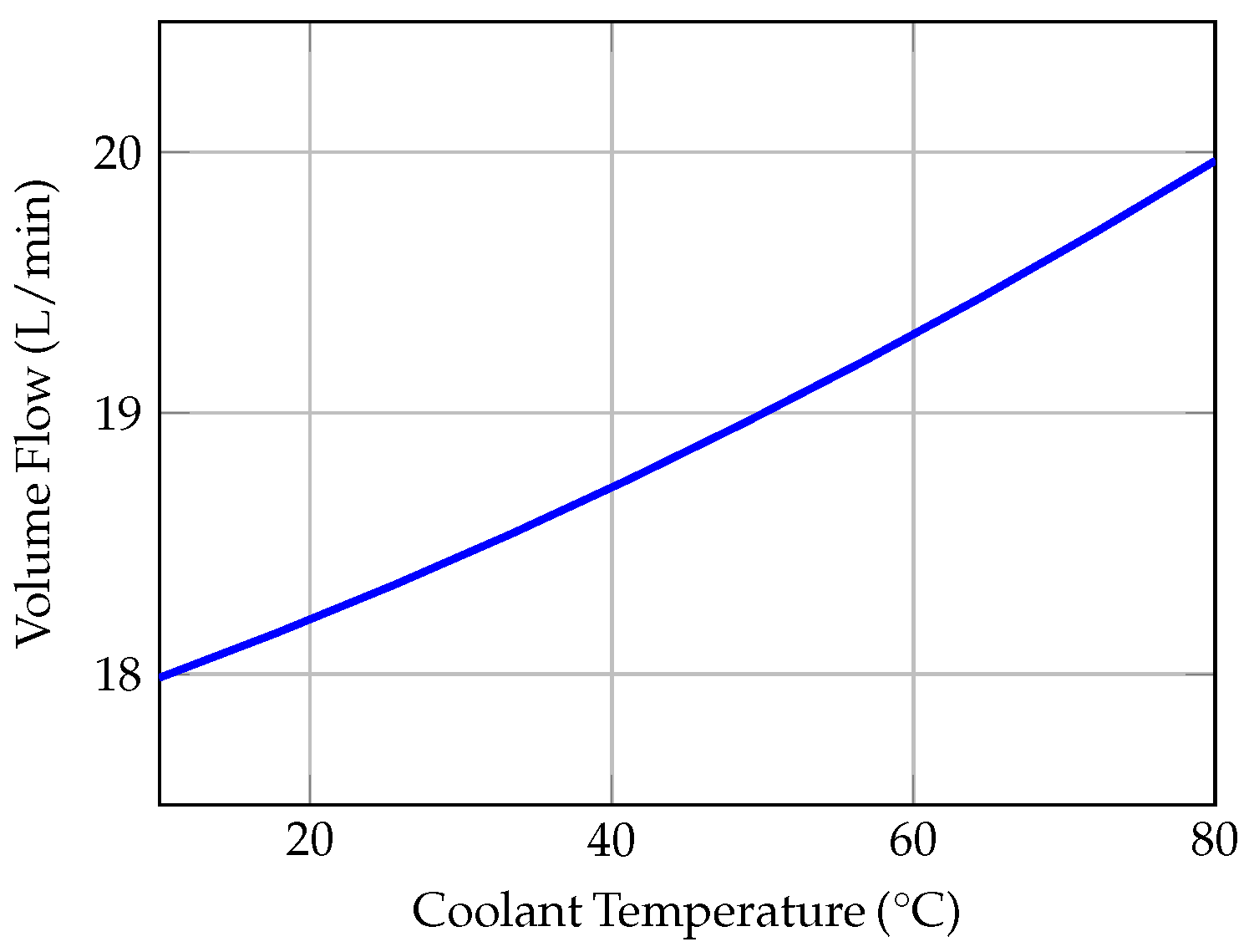
Since the maximum power consumption of the pump ($180\mathrm{W}$) is negligible compared to the maximum heater power ($12\mathrm{kW}$), the pump is operated at maximum speed whenever it is switched on. Consequently, variations in the flow rate are primarily caused by temperature-dependent changes in viscosity. The coolant flow rate is therefore determined experimentally using an ultrasonic volume flow sensor. As the sensor measures volume flow, the temperature-dependent relationship between volume flow and mass flow is incorporated into the model by accounting for the coolant density as a function of temperature. The experimentally determined volume flow and its dependence on temperature are shown in Figure 4.

3.1.1. Heat Exchanger Model

The heat transferred across the heat exchanger is determined using the expression in Equation (11), based on the NTU (Number of Transfer Units) method. A detailed derivation can be found in [23].

$$P_{E\text{-}NTU}=C_{min}·\epsilon ·|T_{HX\text{-}in}-T_{ambient}|$$

(11)

The heat capacity rate C of a fluid is defined as

$$C=\dot{m}·c_p$$

(12)

where $\dot{m}$ is the mass flow rate and $c_p$ is the specific heat capacity. The terms $C_{min}$ and $C_{max}$ denote the smaller and larger of the two heat capacity rates (for the hot and cold fluids), respectively:

$$C_{min}=min(C_{hot},C_{cold}),C_{max}=max(C_{hot},C_{cold})$$

(13)

For a cross-flow heat exchanger with both fluids unmixed, the effectiveness $\epsilon$ is calculated using the following correlation [24]:

$$\epsilon =1-exp\left[{\displaystyle \frac{1}{C_r}}·{\left(NTU\right)}^{0.22}·\left(exp[-C_r·{\left(NTU\right)}^{0.78}]-1\right)\right]$$

(14)

Here, $C_r$ is defined as $C_r=\frac{C_{min}}{C_{max}}$, while the NTU is calculated as

$$NTU={\displaystyle \frac{UA}{C_{min}}}$$

(15)

The overall heat transfer coefficient $UA$ is expressed as

$${\displaystyle \frac{1}{UA}}={\displaystyle \frac{1}{U{A}_1}}+{\displaystyle \frac{1}{G_{wall}}}+{\displaystyle \frac{1}{U{A}_2}}$$

(16)

where $U{A}_1$ and $U{A}_2$ are the convective thermal conductances of fluids 1 and 2, respectively, and $G_{wall}$ is the thermal conductance of the separating wall. The convective conductance on each side is defined by

$$U{A}_i={\displaystyle \frac{N{u}_i·{\lambda }_i·A_i}{c_{dim,i}}}$$

(17)

where $N{u}_i$ is the Nusselt number, ${\lambda }_i$ is the thermal conductivity, $A_i$ is the heat transfer area, and $c_{dim,i}$ is the characteristic length for heat exchange.

The Nusselt number ($Nu$) is calculated using Equation (18). The constants $a_i$, $b_i$, and $c_i$, as well as the Reynolds number ($Re$) and Prandtl number ($Pr$) for both fluids, are determined by performing a least-squares regression using measurement data from the heat exchanger with the E-NTU regression tool in Simcenter Amesim [25]. The dependency of the Nusselt number on the Reynolds and Prandtl numbers is expressed by the following equation:

$$N{u}_i=a_i·{R{e}_i}^{b_i}·{P{r}_i}^{c_i}$$

(18)

The Reynolds number depends on the flow conditions, while the Prandtl number characterizes the fluid properties and is independent of flow conditions. Both numbers are calculated using the formulas provided by the Amesim Regression Tool.

$$Re={\displaystyle \frac{\dot{m}·d_h}{\mu ·S}}$$

(19)

$$Pr={\displaystyle \frac{\mu ·c_p}{\lambda }}$$

(20)

where:

• $d_h$ is the hydraulic diameter
• $\dot{m}$ is the mass flow rate
• $\mu$ is the dynamic viscosity
• S is the cross-sectional area
• $\lambda$ is the thermal conductivity

Calculating the Nusselt number allows the determination of the $NTU$ value in the next step. Using the computed $NTU$, the effectiveness $\epsilon$ of the heat exchanger can be obtained from Equation (14). Finally, Equation (11) is used to calculate the actual heat transferred based on the maximum possible heat exchange. Assuming ideal conditions (i.e., no heat losses and perfect insulation, consistent with the first law of thermodynamics), it can be considered that both the hot and cold fluids exchange the same amount of heat. Under this assumption, the outlet temperature of the coolant can be calculated using Equation (9), while the temperature increase of the air flowing through the heat exchanger is determined using Equation (21).

$$T_{air\text{-}HX\text{-}out}=T_{amb}+{\displaystyle \frac{P_{E-NTU}}{{\dot{m}}_{air}·c_{p,air}}}$$

(21)

3.1.2. Model of the Cabin Volume

The cabin volume is modeled using the heat balance method (HBM), a modeling approach commonly applied in building simulations and presented by the American Society of Heating, Refrigerating, and Air-Conditioning Engineers (ASHRAE) [26]. This approach incorporates three distinct heat balance equations:

• The cabin air volume, assumed to have a uniform temperature $T_{\mathrm{cabin}}$;
• The internal cabin wall temperature $T_{\mathrm{in}}$;
• The external cabin wall temperature $T_{\mathrm{ext}}$.

This layered modeling approach enables improved representation of external heat flows affecting the cabin, including solar radiation and convective heat transfer with the ambient air.

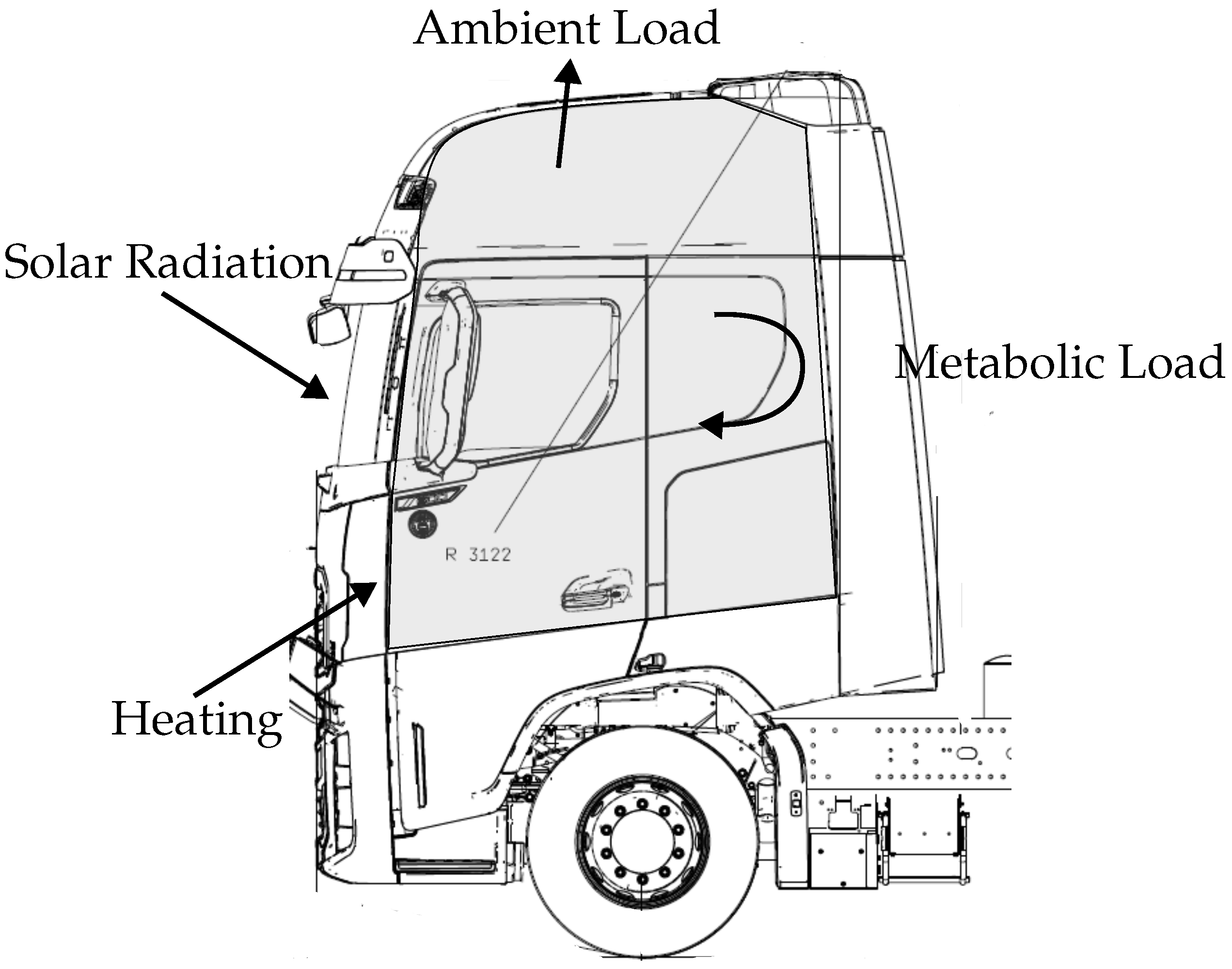
Figure 5 represents the thermal loads affecting the thermal balance of a vehicle cabin.

The thermal loads affecting vehicle cabin are as follows:

• Metabolic Load
  Vehicle occupants produce heat as a result of their metabolic processes. This is considered in the metabolic load modeling. The contribution of this load is relatively small, since physical activity levels are low during driving. Nevertheless, it is included for the sake of completeness in the model. According to ISO 7730 [28], the metabolic rate for a seated person driving is considered constant at $70{\mathrm{W}/\mathrm{m}}^2$. Assuming an average body surface area of $1.8{\mathrm{m}}^2$ [29], the total metabolic load can be calculated using the following equation:

  $${\dot{Q}}_{met}=70{\mathrm{W}/\mathrm{m}}^2·1.8{\mathrm{m}}^2=126\mathrm{W}$$

  (22)
• Ambient Load
  The ambient load describes the heat transfer between the cabin and the environment. In heating mode, heat is transferred from the cabin to the environment, while in air conditioning mode, the direction is reversed. The heat transfer can be separated into the following contributions:

  -

  Heat convection between cabin air and the inner wall, calculated as:

  $${\dot{Q}}_{conv\text{-}int}=(T_{cab}-T_{int})·h_{in}·S$$

  (23)

  where $h_{in}$ is the internal heat transfer coefficient, assumed constant since the blower settings of the HVAC unit remain unchanged.

  S denotes the convective heat transfer surface area obtained from the cabin model.

  -

  Heat conduction from the inner wall to the external wall, expressed as:

  $${\dot{Q}}_{cond\text{-}ext}=(T_{int}-T_{ext})·{\displaystyle \frac{{\lambda }_{wall}}{{\delta }_{wall}}}·S$$

  (24)

  where ${\lambda }_{wall}$ is the thermal conductivity of the cabin walls and ${\delta }_{wall}$ is the wall thickness.

  -

  Heat convection from the external wall to the ambient air, given by:

  $${\dot{Q}}_{conv\text{-}ext}=(T_{ext}-T_{amb})·h_{ext}·S$$

  (25)

  where S denotes the convective heat transfer surface obtained from the cabin CAD model, and $h_{ext}$ is the external heat transfer coefficient. This coefficient is strongly influenced by the air velocity around the vehicle (or the vehicle speed). The convective heat transfer coefficient is modeled as a function of vehicle speed [30]:

  $$h_{ext}=0.6+6.64·\sqrt{V_{veh}}$$

  (26)

• Solar Radiation Load
  Various approaches exist in the literature for modeling solar radiation heat loads. Some studies rely on experimental data [31], while others estimate solar irradiance and sun position based on weather forecasts or historical data [32].
  The radiation load on a surface is calculated as:

  $${\dot{Q}}_{rad}=I·S·cos\left(\theta \right)$$

  (27)

  where:

  -

  I is the solar irradiance,

  -

  $\theta$ is the incident angle, defined as the angle between the sun’s rays and the surface normal,

  -

  S is the surface area.

  The incident solar radiation on a surface can be divided into three components: absorption, reflection, and transmission [33]. Since the reflected component does not directly affect the cabin heat balance, it is neglected in the model. For external walls, solar radiation is primarily absorbed and is calculated using an absorption coefficient $\alpha$, as shown in Equation (28). For windows, solar radiation is predominantly transmitted through the glass, directly impacting the inner walls. This effect is quantified using a transmission factor $\tau$, as shown in Equation (29).

  $${\dot{Q}}_{rad\text{-}\alpha }=I·cos\left(\theta \right)·S·\alpha$$

  (28)

  $${\dot{Q}}_{rad\text{-}\tau }=I·cos\left(\theta \right)·S·\tau$$

  (29)
• Heating Load
  The heat input into the cabin from the heating system is calculated as:

  $${\dot{Q}}_{heater}={\dot{m}}_{air}·c_{p,air}·(T_{air\text{-}HX\text{-}out}-T_{cabin})$$

  (30)

  where $T_{air\text{-}HX\text{-}out}$ is the temperature of the air entering the cabin after passing through the heat exchanger, calculated using Equation (21).

3.1.3. Heat Balance Equations for Thermal Masses in the Cabin

After defining all relevant heat flows, the next step in the modeling process is to establish the heat balance equations for all thermal masses. Although the heat transfer to the ambient is modeled here for the heating scenario, the equations are formulated in a general manner, making them equally applicable to the air-conditioning scenario.

The cabin air temperature, $T_{cab}$, is assumed to be uniform throughout the cabin volume. The heat balance for the cabin air volume is expressed as:

$${\displaystyle \frac{d{T}_{cab}}{dt}}={\displaystyle \frac{1}{V_{air}·{\rho }_{air}·c_{p,air}}}·({\dot{Q}}_{heater}+{\dot{Q}}_{met}-{\dot{Q}}_{conv\text{-}int})$$

(31)

Here, $V_{air}·{\rho }_{air}·c_{p,air}$ represents the thermal mass of the cabin air.

The heat flows affecting the cabin air are as follows:

• ${\dot{Q}}_{heater}$—heat input from the heating system, Equation (30)
• ${\dot{Q}}_{met}$—metabolic heat generation of the driver, Equation (22)
• ${\dot{Q}}_{conv\text{-}int}$—heat transfer between cabin air and internal wall, Equation (23)

The heat balance for the inner wall is expressed as:

$${\displaystyle \frac{d{T}_{int}}{dt}}={\displaystyle \frac{1}{m_{int}·c_{p,int}}}·({\dot{Q}}_{cond,int}+{\dot{Q}}_{rad\text{-}\tau }-{\dot{Q}}_{cond\text{-}ext})$$

(32)

The heat flows considered in the inner wall heat balance are as follows:

• ${\dot{Q}}_{conv\text{-}int}$—heat transfer between cabin air and internal wall, Equation (23)
• ${\dot{Q}}_{cond\text{-}ext}$—heat transfer from the inner wall to the external wall, Equation (24)
• ${\dot{Q}}_{rad\text{-}\tau }$—solar radiation transmitted through the windows, Equation (29)

The heat balance for the external wall is expressed as:

$${\displaystyle \frac{d{T}_{ext}}{dt}}={\displaystyle \frac{1}{m_{ext}·c_{p,ext}}}·({\dot{Q}}_{rad\text{-}\alpha }+{\dot{Q}}_{cond\text{-}ext}-{\dot{Q}}_{conv\text{-}amb})$$

(33)

The heat flows considered in the external wall heat balance are as follows:

• ${\dot{Q}}_{rad\text{-}\alpha }$—heat absorbed from solar radiation, Equation (28)
• ${\dot{Q}}_{cond\text{-}ext}$—heat transferred from the inner wall to the external wall, Equation (24)
• ${\dot{Q}}_{conv\text{-}amb}$—heat transferred between external wall and environment, Equation (25)

3.1.4. Extension of the Model for Coupling with Cooling Circuit

As illustrated in Figure 3, the heating circuit is coupled via a three-way valve with a middle-temperature (MT) cooling circuit operating at approximately 40–60 °C. This cooling circuit manages the temperature of the drivetrain components (motors, inverters, transmission), DC/DC converters, air compressor, fuel cell power electronics, and the on-board charger (OBC). Coupling the circuits in the simulation allows evaluating the effectiveness of the MPC in managing multi-input multi-output (MIMO) systems.

For simplification, the cooling system is modeled with a constant coolant temperature of 40 °C, representing a worst-case scenario for heating due to the low coolant temperature. A simulation of the MT cooling circuit using a dedicated model, the details of which are beyond the scope of this investigation, showed that the coolant temperature remains nearly constant after the initial heating phase (<3% of the driving cycle). In this simulation, the temperature was successfuly controlled to 40 °C, as exceeding 45 °C would trigger derating of the electric motor. This confirms that the assumption of a constant 40 °C is reasonable for evaluating MPC performance. The valve regulates the volume flow between the heating and cooling systems by adjusting its position. The resulting coolant temperature entering the HV heater is calculated algebraically using an energy balance between the heating system and the cooling system:

$$T_{H\text{-}in,eff}=(1-w_{valve})·T_{H\text{-}in}+w_{valve}·T_{waste}$$

(34)

Here, $T_{H\text{-}in,eff}$ represents the effective coolant temperature entering the heater (Equation (9)), $w_{valve}$ denotes the valve position ($w_{valve}=1$ when fully open, $w_{valve}=0$ when closed), $T_{H\text{-}in}$ is the temperature calculated in Equation (8), and $T_{waste}$ is the temperature of the coolant returning from the drivetrain cooling system.

Although this approach significantly simplifies the cooling system by assuming a constant coolant temperature, it still provides valuable insights into two key aspects: the potential use of drivetrain waste heat for cabin heating, and the effectiveness of the MPC controller in handling MIMO systems.

3.1.5. Thermal Comfort Calculation

Thermal comfort is subjective and dependent on both environmental conditions and individual sensations. It is not merely influenced by temperature, but also by relative air humidity, mean radiant temperature, and air velocity. One of the most common methods for evaluating thermal comfort in the automotive field is the PMV method proposed by Fanger [29]. Its applications range from localized thermal comfort assessments under specific operating conditions, where the cabin is represented as a 3D model and PMV is computed spatially [34], to its integration into HVAC control strategies for optimizing occupant comfort. The PMV index is assessed on a seven-point scale ($-3$: cold, $-2$: cool, $-1$: slightly cool, 0: neutral, $+1$: slightly warm, $+2$: warm, $+3$: hot), with 0 representing neutral conditions where most humans would feel comfortable.

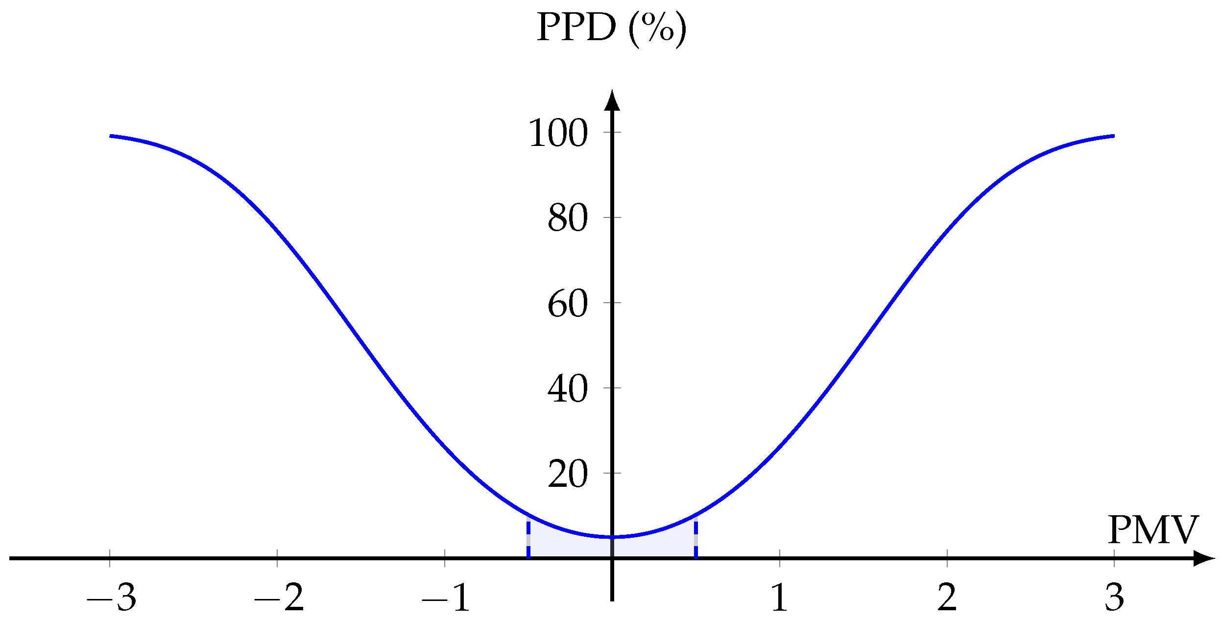
Closely linked to PMV is the Predicted Percentage of Dissatisfied (PPD) index, which is not independent but mathematically derived from PMV. It quantifies the expected share of people dissatisfied with the thermal environment at a given PMV value, according to the following relation [35]:

$$\mathrm{PPD}=100-95·exp(-0.03343·{\mathrm{PMV}}^4-0.2179·{\mathrm{PMV}}^2)$$

(35)

This relationship is nonlinear: even at PMV = 0, at least 5% of people are predicted to feel uncomfortable, and the PPD increases sharply as PMV deviates from neutral. A PPD value of 10% (corresponding approximately to PMV between $-0.5$ and $+0.5$) is usually considered the acceptable threshold for a comfortable thermal environment, as illustrated in Figure 6.

Both the ASHRAEand ISO 7730 thermal comfort standards define thermal comfort assessment using the PMV index. A common feature of both standards is that they provide pseudo-code outlining the calculation procedure for the PMV index [28,35]. In this study, the PMV calculation is implemented in a MATLAB Simulink model, based on the pseudo-code provided in these standards. The Simulink model is organised into three main parts. The first part defines the input parameters required for the PMV calculation, including the computation of relative humidity as a function of the cabin temperature. The second part performs the iterative calculation of the clothing surface temperature using the equations specified in the standards. Finally, the third part computes the PMV index.

In

Table 2. Parameters used for the calculation of PMV.

Parameter	Value
Metabolic rate	$M=70$ W/m2 (driving) [28]
Effective mechanical power	$W=0$ W/m2 (no physical effort) [28]
Clothing insulation	$I_{cl}=1$ clo (typical winter clothes) [28]
Water partial pressure	Equation (36)
Mean radiant temperature	${\overline{t}}_r=T_{int}$ Section 3.2.3
Air velocity	${\overline{v}}_{air}=0.3754$ m/s Section 3.2.3

, the values of the parameters chosen for the PMV calculation are presented. The choice of the parameter values was made with the tables present in the ISO norm 7730 [28].

The partial pressure of water vapor is determined using the relative humidity and the saturation vapor pressure, as shown in Equation (36). The saturation vapor pressure can be estimated with the Tetens equation [36]. Equation (37) illustrates this calculation.

$$p_a=RH·p_{sat}$$

(36)

$$p_{sat}=611.2·exp\left({\displaystyle \frac{17.27·T}{T+237.7}}\right)$$

(37)

where:

• $RH$ is the relative humidity,
• T is the ambient temperature.

Because there is no relative humidity sensor in the vehicle cabin, this value must be estimated from the temperature. The estimation assumes that the water vapor partial pressure remains constant. The initial water vapor partial pressure is calculated using the relative humidity, and for subsequent states, it is estimated based only on temperature. The accuracy of this approach should be assessed using experimental data; see Section 3.2.3. If the results are not sufficiently precise, other methods may be considered, such as applying a different correlation or installing a humidity sensor in the cabin. The initial water vapor pressure can be determined using Equations (36) and (37), and the relative humidity (as a percentage) for a given cabin temperature T is calculated as follows.

$$RH={\displaystyle \frac{p_a\left(T_{\mathrm{start}}\right)}{p_{\mathrm{sat}}\left(T\right)}}·100$$

(38)

The air velocity and mean radiant temperature within a vehicle cabin can vary significantly depending on location. For instance, the air speed at head and torso level often differs from that near the feet. Similarly, the mean radiant temperature is affected by factors such as solar exposure and surface temperatures of the interior, leading to spatial variations. Although cabin models typically assume uniform temperature distributions, these spatial differences in air velocity and radiant temperature should be considered when evaluating thermal comfort. ISO 7730 addresses this by recommending measurements in non-uniform environments at multiple heights, specifically, at three levels with results averaged as summarized in

Table 3. Recommended measurement heights for sitting and standing positions according to ISO 7730.

Position	Sitting	Standing
Head level	1.1 m	1.7 m
Abdomen level	0.6 m	1.1 m
Ankle level	0.1 m	0.1 m

.

The mean radiant temperature in a vehicle cabin is affected by several factors, including cabin air temperature, the temperature of interior surfaces, and incoming solar radiation. To better understand how these variables are correlated, targeted measurements will be conducted (see Section 3.2.3).

The blower settings of the HVAC system will be kept constant to maintain a steady air velocity. For accurate thermal comfort analysis, air velocity will be measured at three specified heights, and these measurements will be averaged to determine the mean air velocity, ${\overline{v}}_{air}$.

3.2. Experimental Setup and Data Acquisition

To enable fast calculations suitable for Model Predictive Control (MPC), considerable simplifications were made when modeling the vehicle cabin. A series of experiments were conducted to verify that these simplifications did not introduce significant errors. This validation is especially important because exact values of some heat transfer coefficients are difficult to calculate, often requiring reliance on approximate or literature values.

Given the hypothesis that the mean radiant temperature can be approximated by the temperature of surrounding surfaces ($T_{int}$), PMV-related measurements were performed. Sensors were installed at various locations throughout the cabin to collect relevant data. These measurements were also essential for acquiring realistic air velocity data. Furthermore, the simplified relative humidity calculation required validation. Lastly, PMV measurements were used to analyze the impact of cabin inhomogeneity on PMV parameter values. An overview of the sensor positions inside the vehicle cabin is shown in Figure 7.

A summary of the sensors used, along with their measurement purposes and accuracies, is provided in

Table 4. Overview of sensors used for experimental validation of simulation models.

Sensor	Measurement Purpose	Accuracy
PT1000 Class A	Air temperature	±(0.15 $\mathrm{°C}+0.002\left|t\right|)$
Type K thermocouple	Surface temperature	±1.5 °C
Capacitive polymer sensor	Air humidity	±2% RH
Silicon radiation sensor	Solar irradiance	±5 W/m2
Black globe thermometer	Radiation temperature	±(0.15 $\mathrm{°C}+0.002\left|t\right|)$
Omnidirectional anemometer	Air velocity	±0.03 m/s (0.05–1 m/s); ±3% of reading (1–3 m/s)
Ultrasonic sensor	Volumetric flow rate	±3 % of reading

.

Data acquisition was performed using a modular Q.brixx system from Gantner [37]. Three XL A107 measurement modules, each featuring four multifunctional analog inputs, were utilized. In total, the following three experiments were conducted to provide a basis for model validation:

• Heating system validation
• Solar radiation–related measurements
• PMV-related measurements (including air velocity and air humidity measurements)

3.2.1. Heating System Validation

The heating system validation experiment was performed on a cold winter day after sunset to eliminate the influence of solar radiation. The heater power was kept constant at $5\mathrm{kW}$ to enable a more straightforward comparison between simulation and measurement. Under these conditions, the only significant heat loads acting on the cabin were the metabolic load, the heating system itself, and heat losses to the ambient environment.

The experiment was carried out with the vehicle in a stationary state and the HVAC system operating in heating mode. The ambient air temperature, interior and exterior surface temperatures, and cabin air temperature were recorded using temperature sensors placed at representative positions inside and outside the cabin. The inner wall temperatures were measured at several heights near the driver’s position and subsequently averaged. The ambient temperature sensor was positioned away from any local heat sources to ensure undistorted measurements.

The chosen constant heating power allowed the thermal response of the cabin to be observed without interference from fluctuating control inputs. This approach simplified the identification of thermal parameters, such as the internal and external convection coefficients, the thermal conductivity of the cabin wall, and the thermal masses of key components. The resulting data formed the basis for parameter estimation in the simulation model, ensuring that the simulated temperature profiles could be matched to the experimental results with minimal deviation.

3.2.2. Solar Radiation Validation

Following the heating system test, a second experiment was conducted to isolate and quantify the effects of solar radiation on the cabin thermal loads. This test was performed with the heating system turned off to exclude its influence, allowing the thermal impact of solar radiation alone to be observed.

Measurements included ambient air temperature, exterior and interior surface temperatures of the cabin, as well as cabin air temperature. Solar radiation was recorded using a sensor insensitive to the angle of incidence, which was suitable given that the vehicle remained stationary throughout the test and the relative positions of the surfaces did not change. The sun’s position during the test was determined using historical solar data.

3.2.3. PMV Measurements

For the PMV measurements, the primary objective was to obtain data for thermal comfort assessment, including parameters such as air velocity. As highlighted in Section 3.1.5, while the PMV calculation assumes homogeneous environmental conditions, ISO 7726 [38] also allows the inclusion of inhomogeneous data. This method involves measuring environmental parameters at three standardised heights and calculating their mean values.

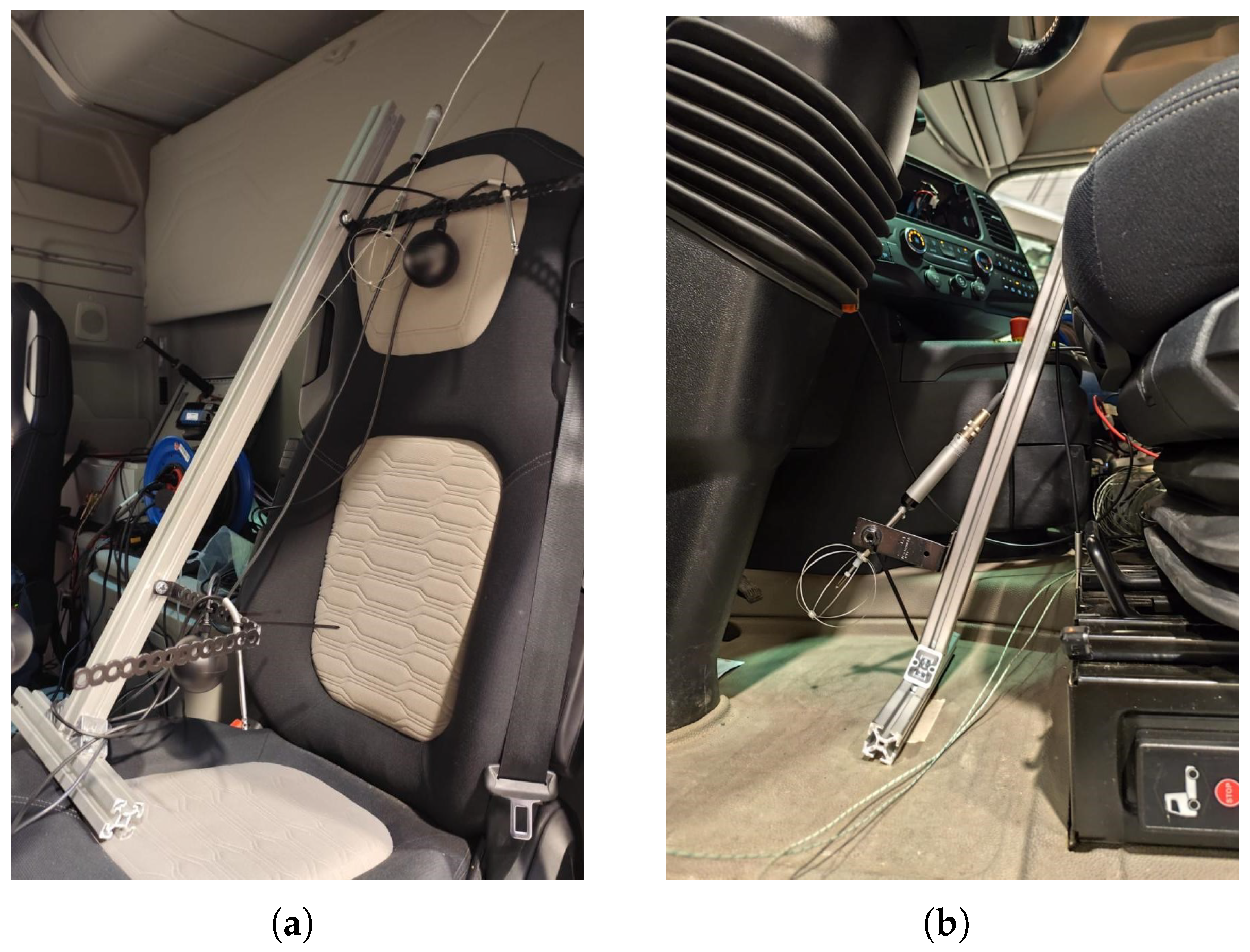
To achieve this, a measurement stand was constructed to facilitate data collection at the three heights specified by ISO 7726, as shown in Table 3. A photo of the stand built for the measurements is provided in Figure 8. Also visible in the photos are the Swema air velocity sensors and the black globe thermometers used for determining the mean radiant temperature.

Since the HVAC blower settings were kept constant throughout the test, the air velocities inside the cabin were also expected to remain relatively stable over time. The air velocity was measured at the three standardised heights during three different tests. The time-averaged values from each height were then computed, and the mean air velocity around the driver’s body was determined for the PMV calculation.

For the measurement of air velocity, an omnidirectional probe (Swema 03) compliant with ISO 7730 was used. It is capable of detecting the velocity magnitude independent of direction.

It was previously decided not to measure relative humidity directly and to treat it as a measured disturbance. Instead, a simple calculation method was introduced in Section 3.1.5. This calculation method must be validated against measurements to ensure that it can accurately reproduce the behavior of relative humidity.

For this purpose, a Telaire T9602 humidity and temperature sensor was installed at head height. Using the same sensor for both temperature and humidity improves the accuracy of the relative humidity measurement.

3.3. Model Validation

This section presents the validation of the developed simulation models using experimental data. The aim is to demonstrate that the models accurately represent the physical behavior of the cabin thermal system under various conditions.

3.3.1. Air Velocity Measurements

To characterize the airflow conditions within the cabin, air velocity measurements were performed at three representative heights corresponding to the head, abdomen, and ankle levels (see Table 3). The measured velocities were averaged over the measurement period and are summarized in

Table 5. Measured air velocities at different heights.

Position	Velocity [m/s]
$v_{air\text{-}Head}$	$0.2386$
$v_{air\text{-}Abdomen}$	$0.5830$
$v_{air\text{-}Ankle}$	$0.3046$

.

These measured velocities serve as input parameters for the thermal comfort model and contribute to the calculation of convective heat transfer and PMV estimations in the simulation. While no direct comparison with simulation results is performed here, these values ensure that the modeled airflow conditions realistically reflect the experimental environment.

3.3.2. Relative Humidity Measurements

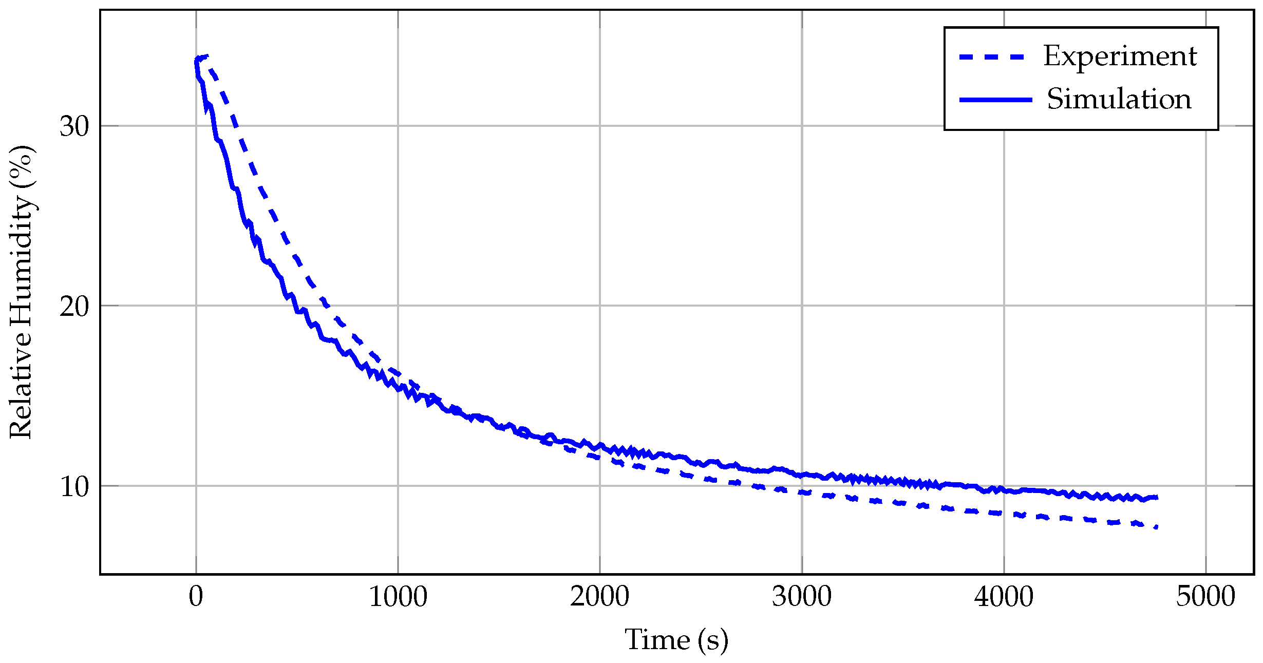
The data obtained in the experiment described in Section 3.2.3 are compared with simulation results. The measured and calculated values are shown in Figure 9.

Since the comparison shows deviations of no more than 3% between the measured and calculated relative humidity values, the approach can be considered valid and sufficient. Therefore, no sensor for relative humidity is required to implement this variable as a measured disturbance.

3.3.3. Mean Radiant Temperature

Similar to the air velocity measurements, the mean radiant temperature (MRT) was recorded using black globe thermometers positioned at three different heights. When calculating the average radiation temperature, it is commonly assumed to be comparable to the air temperature measured with a standard PT1000 sensor or approximated by the interior wall temperature, which represents radiation from the surrounding surfaces.

To verify these assumptions, measurements from the two experiments described in Section 3.2, one conducted without solar radiation and one conducted with solar radiation, were analyzed. The first experiment allows verification of the correlation between MRT and air or interior wall temperatures under baseline conditions, while the second experiment provides insight into how solar radiation influences MRT.

When measuring temperature with black globe thermometers, ISO 7726 [38] recommends a correction to eliminate the influence of convective heat transfer with the environment. This correction is applied using the following formula:

$$\overline{t}r={\left[{(t_g+273)}^4+{\displaystyle \frac{1.1·{10}^8·v{air}^{0.6}·(t_g-t_a)}{{\epsilon }_g·D^{0.4}}}\right]}^{1/4}-273$$

(39)

• ${\epsilon }_g$ is the emissivity of the black globe (${\epsilon }_g=0.95$ for matte black surfaces)
• $v_{air}$ is the air velocity
• $t_g$ is the measured globe temperature
• $t_a$ is the measured air temperature
• D is the diameter of the sphere

Due to the blower configuration during testing, which directed all airflow toward the windshield, noticeable differences in average radiant temperature were observed across different vertical levels. As illustrated in Figure 10, the radiant temperatures at head and torso levels are relatively similar, whereas the value at foot level is considerably lower. These observations further highlight the need to account for non-uniform conditions in the thermal comfort evaluation to avoid overlooking discomfort in specific body regions.

3.3.4. Heating System

The essential part of the simulation model for ensuring robust control is the heat transfer from the coolant to the interior air. To validate the suitability of the model, the coolant temperatures before and after the heater, the coolant mass flow, and the air temperature entering the interior must be compared with measurements. For the coolant temperatures, the measurements available via vehicle CAN communication within the HV heater were used. Losses through the hoses and pipes are neglected, so that the temperature at the outlet of the HV heater corresponds to the temperature at the inlet of the heat exchanger. The volume flow was measured with an ultrasonic flow sensor from Keyence attached to one of the hoses.

By analyzing the steady state, the heat transfer characteristics of the heater and the heat exchanger can be accurately validated. To achieve a steady state, the heating power was set to a constant value of $5\mathrm{kW}$. Since the speed of the water pump does not vary, the hydraulic losses in the system were not modeled. Instead, the volume flow is calculated as a function of the coolant temperature, for which a characteristic curve was created based on measurements.

The results of the coolant temperatures with a constant heating output of 5 kW are shown in Figure 11. As can be seen, the model accurately predicts the coolant temperatures, with deviations of less than 1 °C. Considering that the accuracy of the available temperature measurements in the heater is approximately 1 °C, this represents a satisfactory match.

The recorded data from the same experiment were also used to validate the air temperature at the outlet of the heat exchanger and at the inlet to the cabin. The temperatures were measured with two PT1000 sensors installed in the ventilation opening of the HVAC system. Figure 12 compares the air temperature at the outlet of the heat exchanger in the measurements and in the simulation. Since the sensors used here are more accurate, the model predictions are even closer to reality. The slightly higher temperatures observed in the experimental data may be due to the warming effect of nearby components such as hoses and expansion tanks located near the air intake point.

3.3.5. External Heat Loads

The most challenging part of the model is capturing the external heat loads due to the simplifications involved. For example, representing the cabin air volume as a single thermal mass is a significant simplification, since inhomogeneities occur in reality. The aim of validating this part of the model is to ensure that these effects on the heating system are represented realistically.

The validation of heat loads acting on the interior considers both the heat input from solar radiation and the heat loss to the environment. Since these two loads act simultaneously, they are evaluated separately. Accordingly, the validation is carried out in two steps. In the first step, data from tests without solar radiation are analyzed; in the second step, solar radiation is included.

The heat loss to the environment consists of three components, all of which are validated by measurements. The convective heat transfer between the cabin air and the interior walls is evaluated by measuring the temperature difference between the cabin air and the interior wall. Two surface temperature measurements are used to assess heat conduction through the cabin walls. Finally, heat transfer from the walls to the ambient air is evaluated based on the temperature difference between the ambient air and the outer wall. Surface temperatures were measured with type K thermocouples placed in direct contact with the surfaces. The inner wall temperatures were measured near the driver’s position at various heights and then averaged.

The first test was carried out after sunset to exclude the influence of solar radiation. The two remaining loads acting on the cabin are the heat input from the high-voltage heating system, kept constant at $5\mathrm{kW}$, and the heat loss to the environment. The heat loss consists of three components: $Q_{conv\text{-}int}$, determined by the internal convection coefficient $h_{in}$; $Q_{cond\text{-}ext}$, determined by the ratio of thermal conductivity to wall thickness, ${\displaystyle \frac{{\lambda }_{wall}}{{\delta }_{wall}}}$; and $Q_{conv\text{-}ext}$, determined by the external convection coefficient $h_{ext}$. The following temperatures were recorded for validation: ambient air temperature, exterior and interior surface temperatures of the cabin, and cabin air temperature. The aim was to estimate the heat transfer coefficients for internal and external convection, the thermal resistance of the cabin walls, and the thermal masses of various components in order to match the simulated temperature profiles with the experimental data.

Heat transfer coefficients are challenging to model because they are influenced by many factors. For this reason, the Simulink Parameter Estimation Tool was used to adjust these parameters so that the model matches reality. The final results of this process are shown in Figure 13. The results are highly satisfactory, with deviations between simulation and measurement of less than 1 °C on average.

After completing the test with the heating system, another test was conducted to quantify the effects of solar radiation. This test was performed without activating the heating system in order to isolate the effect of solar radiation. The radiation absorption factor $\alpha$ and the transmission factor $\tau$ were used to correlate the model with the experimental values and to account for the simplifications in the calculation of $Q_{rad}$. The temperature measurements included ambient temperature, exterior and interior surface temperatures, as well as the cabin air temperature. The sensor used to measure solar radiation is insensitive to the angle of incidence; however, since the vehicle was stationary, the positions of the vehicle surfaces remained constant. The position of the sun was determined from historical data.

As shown in Figure 14, the positioning of the temperature sensors has a significant impact on the measurements. Although the sensors in the cabin air and on the interior wall initially display similar values, a clear difference emerges when exposed to sunlight. This is because the interior wall temperature is measured above the driver’s head, where it receives little direct sunlight, whereas the sensor near the driver’s head is directly exposed to sunlight. Although heat convection occurs between the interior wall and the cabin air, it is not sufficient to equalize the temperatures.

Two possible explanations exist for these discrepancies. First, inhomogeneity of the cabin air could account for the temperature difference. Second, solar radiation may directly influence the temperature measurement by heating the sensor itself. This is plausible, as a sharp drop in temperature was observed as soon as the solar radiation was removed.

To estimate the parameters $\alpha$ and $\tau$, the following approach was implemented: Since it was observed that, after the initial influence of solar radiation, both the cabin and interior wall temperatures tend to converge to similar values, it was assumed that in a distributed system, the homogeneous cabin air temperature should converge to these values. Knowing the temperature after the first solar radiation exposure, the parameters $\alpha$ and $\tau$ can be estimated. The comparison between the model calculations and the experimental data is shown in Figure 14.

3.3.6. Repeatability of Experimental Results

Each heating experiment was repeated three times ($n=3$). While environmental conditions such as ambient temperature, solar radiation, and wind varied slightly between runs, the simulation consistently captured the system behavior.

Table 6. Average RMSE between simulation and experiment, and standard deviation of repeated experiments for different measured variables.

Variable	Average RMSE [unit]	Standard Deviation [unit]
Relative humidity	1.426 [%]	0.100 [%]
Heater inlet temperature	0.558 [°C]	0.114 [°C]
Heater outlet temperature	1.427 [°C]	0.119 [°C]
Heat exchanger outlet temperature	0.346 [°C]	0.078 [°C]
Outer wall temperature	0.150 [°C]	0.410 [°C]
Inner wall temperature	0.338 [°C]	1.429 [°C]
Cabin air temperature	0.877 [°C]	0.252 [°C]

reports the root mean square error (RMSE) between the simulation and each experiment, along with the standard deviation across the three runs. The RMSE provides a measure of the deviation between the simulated and measured values. These results highlight that the simulation reliably reproduces the measured dynamics despite variations in the experimental conditions.

3.4. Formulation of the Optimization Problem

To implement MPC in Simulink, the associated optimization problem must first be defined. This involves specifying the optimization objective by formulating an appropriate cost function. The system dynamics are represented using state variables, while control over the system is exerted through manipulated variables (MVs). External influences on the system behavior are treated as measured disturbances (MDs).

Within the cabin thermal model, the state variables X represent the temperatures governed by the five heat balance equations of the system. The system output Y is defined as a function of these state variables. The input vector U comprises both measured disturbances and the manipulated variable, which in this study is the heating power $P_H$. The categorization of these signals is presented in Equation (40).

$$X=\left[\begin{array}{c}{x}_1\\ x_2\\ x_3\\ x_4\\ x_5\end{array}\right]=\left[\begin{array}{c}{T}_{cab}\\ T_{H\text{-}in}\\ T_{HX\text{-}in}\\ T_{int}\\ T_{ext}\end{array}\right],U=\left[\begin{array}{c}{u}_1\\ u_2\\ u_3\\ u_4\\ u_5\\ u_6\\ u_7\\ u_8\end{array}\right]=\left[\begin{array}{c}{I}_{solar}\\ {\dot{Q}}_{met}\\ T_{amb}\\ V_{veh}\\ PW{M}_{WP}\\ P_H\\ v_{air\text{-}R}\\ v_{air\text{-}PMV}\end{array}\right],Y=\left[\begin{array}{c}{y}_1\\ y_2\\ y_3\\ y_4\\ y_5\end{array}\right]=\left[\begin{array}{c}{T}_{cab}\\ T_{H\text{-}in}\\ T_{HX\text{-}in}\\ T_{int}\\ T_{ext}\end{array}\right].$$

(40)

The input vector U includes varying external MDs such as solar irradiance ($u_1=I_{solar}$), ambient temperature ($u_3=T_{amb}$), and vehicle velocity ($u_4=V_{veh}$). Additionally, the metabolic heat load from the passenger ($u_2={\dot{Q}}_{met}$) is modeled as a constant input. The manipulated variable considered in this study is the heater power ($u_6=P_H$). To enable coupling with the cooling system, the valve position ($u_9=w_{valve}$) is also included, as described in Section 3.1.4.

The MPC structure is designed to be extendable with additional MVs, such as pump control ($u_5=PW{M}_{WP}$) to regulate coolant flow in the heating circuit, and two air velocity inputs related to HVAC operation: the air velocity through the heat exchanger ($u_7=v_{air\text{-}R}$) and the average air velocity near the occupant’s body used in the PMV calculation ($u_8=v_{air\text{-}PMV}$).

To ensure that the developed control strategy respects physical and operational boundaries, constraints are introduced. For example, the temperature of the water–glycol mixture is limited as defined in Equation (41):

$$-30\mathit{°C}\le x_2,x_3\le 90\mathit{°C}$$

(41)

The HV electrical heater has a maximum power of $12\mathrm{kW}$, which is enforced in the MPC controller, as shown in Equation (42). A lower power boundary is also introduced to avoid numerical issues when the power approaches zero.

$$0.1\mathrm{W}\le u_6\le 12000\mathrm{W}$$

(42)

It is necessary to limit actuator changes to prevent unphysical variations in the manipulated variables. For this purpose, the rate of change of heating power per time step is constrained, as defined in Equation (43):

$$-3000\mathrm{W}\le \Delta u_6\le +8000\mathrm{W},\mathrm{where}\Delta u_6=u_6\left(k\right)-u_6(k-1)$$

(43)

The implemented possibility of coupling the heating circuit with the middle-temperature (MT) cooling circuit allows evaluation of the MPC’s capability in handling MIMO systems. This implementation introduces a new MV, the valve position, defined as $u_9=w_{valve}$. The valve regulates the coolant volume flow between the cabin heating system and the MT cooling circuit.

This coupling is meaningful only when the outlet temperature of the cabin heat exchanger is lower than the MT coolant temperature; otherwise, more energy would be consumed. The valve position $w_{valve}$ ranges from 0 to 1, where $w_{valve}=0$ represents a fully closed valve, impeding coolant transfer between the systems, and $w_{valve}=1$ represents a fully opened valve, merging both systems into a single circuit.

To ensure system stability and prevent abrupt fluctuations, the rate of change of $w_{valve}$ per controller time step is constrained. The corresponding constraints are as follows:

$$0\le u_9\le 1$$

(44)

$$-0.5\le \Delta u_9\le 0.5,\mathrm{where}\Delta u_9=u_9\left(k\right)-u_9(k-1)$$

(45)

The primary objective of the MPC is to optimize energy consumption while maintaining thermal comfort in the cabin. Energy consumption is quantified by the electrical heater power, whereas thermal comfort is assessed using the PMV index. The MPC is designed to unify and balance these two potentially conflicting goals: maintaining thermal comfort while minimizing energy consumption.

To achieve this, the cost function includes a quadratic penalty term that disproportionately penalizes larger deviations from the desired comfort level. The energy consumption term is formulated as the square of the heater power at each time step, imposing a stronger penalty on higher energy usage. This structure enhances the balance between tracking performance and energy efficiency, providing a flexible and adaptable optimization framework.

As highlighted in Section 3.1.5, an acceptable thermal comfort environment is defined by a PPD of 10%, corresponding to $-0.5\le \mathrm{PMV}\le 0.5$. This range allows the inclusion of a slack variable in the cost function, which penalizes deviations only when the PMV falls outside the defined range.

The cost function consists of three components: the energy usage cost, the PMV deviation cost, and the PMV slack variable. Each component is weighted by a factor that enables prioritization of different elements within the cost function. The defined cost function is shown in Equation (46):

$$J\left(k\right)=\sum _{i=0}^p\left[{\left(u_6(k+i)\right)}^2·R_1+{\left(PMV(k+i)\right)}^2·R_2+{ϵ}_{PMV}(k+i)·R_3\right]$$

(46)

where:

• $R_1$, $R_2$, and $R_3$ are the weighting factors
• $u_6\left(k\right)$ is the heater power
• $PMV$ is the calculated PMV index
• ${ϵ}_{PMV}$ is the PMV slack variable

The slack variable for the PMV penalizes deviations when the absolute value of the PMV exceeds the acceptable range of $\pm 0.5$:

$${ϵ}_{PMV}=max(0,|PMV|-0.5)$$

(47)

The proposed cost function prioritizes maintaining the cabin within an acceptable thermal comfort range over the other objectives. Once this region is reached, the cost function optimally balances thermal comfort and energy consumption. By adjusting the weighting factors, the MPC strategy can be customized to emphasize either thermal comfort or energy efficiency, depending on the desired objective.

To clarify the MPC implementation, the selection of the prediction and control horizons is briefly summarized here. A sensitivity study was conducted to evaluate the effect of the prediction horizon on controller performance, using step sizes of $180\mathrm{s}$ and $300\mathrm{s}$. The prediction horizon p was varied while maintaining a fixed ratio for the control horizon ($c=0.5·p$). The main priority of the MPC was to bring the cabin environment into the acceptable thermal comfort range, after which the controller balanced thermal comfort and energy consumption.

The study showed that a step size of $180\mathrm{s}$ outperforms $300\mathrm{s}$ in responding to sudden changes in external disturbances, with only minor fluctuations in PMV values. Increasing the prediction horizon further improves the MPC’s proactive response, enhancing overall performance without significantly increasing computational demand.

Based on these findings, the combination $T_s=180\mathrm{s}$, $p=25$, and $c=12$ was selected for the simulations. This configuration provides an effective balance between performance, computational efficiency, and robustness against potential model mismatch, making it suitable for realistic vehicle implementation.

4. Results

This section presents the results of the simulations and discusses the conclusions that can be drawn. First, the simulation setup is outlined, including the definition of the driving cycle and the ambient conditions. Next, a traditional PID-based control approach is presented as a benchmark for comparison with MPC. Subsequently, the performance of MPC is compared to the traditional control method to highlight its advantages. Finally, the potential for integrating cabin heating with the MT cooling circuit is discussed.

4.1. Simulation Setup

In this subsection, the ambient conditions, including temperature profiles, and the driving cycles used in the simulations are introduced.

4.1.1. Ambient Conditions

The ambient temperature profile is based on historical data from two winter days in Aachen: 10 January and 27 January 2024. These dates were selected to illustrate two different scenarios. 27 January represents an average winter day in Aachen, aligning with the typical operating conditions of the SeLv truck. 10 January represents an extreme low-temperature scenario for this region, with temperatures reaching −8 °C, which is colder than the typical January average of 0–2 °C. This colder day provides a challenging scenario for evaluating the truck’s thermal management performance. While even colder climates exist, such conditions would require pre-conditioning of the HV battery and/or cabin, as well as different initial conditions, which are beyond the scope of this study.

The temperature variations over both days are illustrated in Figure 15.

4.1.2. Driving Cycles

To assess the performance of the developed controller under realistic driving conditions, two driving cycles were selected. The first cycle was recorded during Project SeLv, while driving through western Germany on both highways and country roads. Details of this cycle have been presented in [39], and it is shown in Figure 16.

To evaluate the controller’s performance under conditions with frequent and abrupt velocity changes, the VECTO urban delivery cycle was selected, shown in Figure 17. VECTO is a simulation tool developed by the European Commission for the calculation of CO₂ emissions and fuel consumption of heavy-duty vehicles [40].

4.2. Tuning of the Weighting Factors

The weighting of variables in the cost function allows prioritization of specific objectives in the MPC optimization process. It can be configured either to maintain the PMV index close to zero for ideal thermal comfort or to minimize energy consumption by operating near the acceptable thermal comfort limits.

In this study, the main goal is to maintain a thermal comfort environment with a PPD below 10% throughout the driving period. Therefore, the highest weight is assigned to the slack variable associated with the PMV, ensuring that it remains within the desired range and that restoring thermal comfort takes precedence over energy consumption whenever deviations occur.

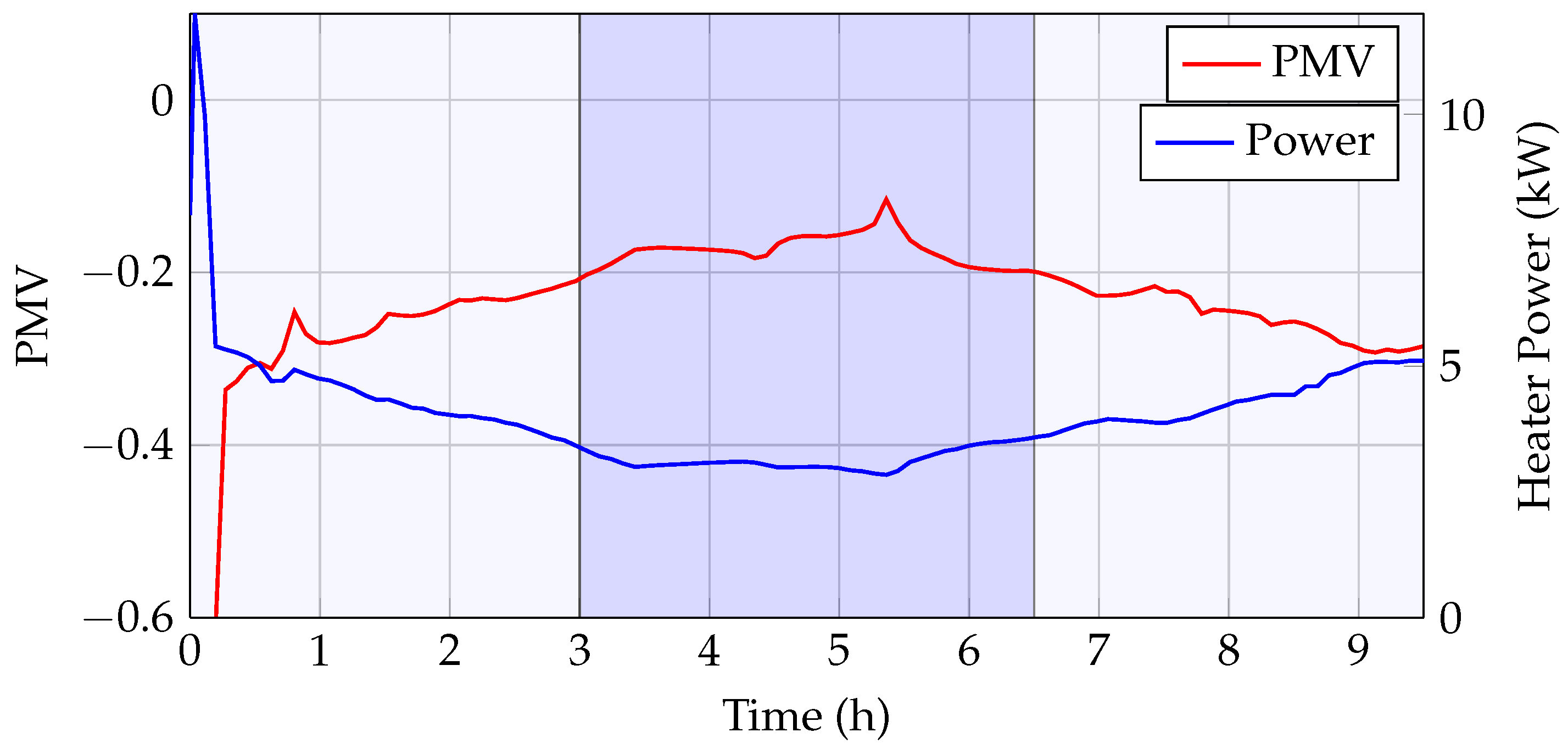
Once the PMV index is within the acceptable range, the MPC balances the remaining factors related to energy consumption and PMV deviation from zero. This approach allows fluctuations within the acceptable thermal comfort region while optimizing energy use. During periods of high energy demand, the MPC may compromise on ideal comfort to reduce energy consumption, whereas during low energy demand, thermal comfort is prioritized. This working principle is illustrated in Figure 18. Light blue regions indicate high energy demand where comfort may be slightly compromised to decrease energy usage, while dark blue regions represent low energy demand phases where thermal comfort is prioritized.

A series of simulations was conducted using different weighting factors, resulting in varying average PMV values. Ultimately, a set of factors was selected that yields a slightly compromised average PMV of $-0.2$ while achieving significant energy savings. The chosen weighting factors are listed in

Table 7. Weighting factors defined for the MPC cost function through simulation.

Factor	Value
$R_1$	$0.000037$
$R_2$	1000
$R_3$	5000

4.3. Simulation Results

The performance of the Model Predictive Controller (MPC) is benchmarked against a conventional PID controller. The evaluation criteria for MPC include the PMV and total energy consumption throughout the driving cycle. The PID controller can maintain a set PMV value but does not consider energy demand. In contrast, MPC provides the additional capability of pursuing multiple objectives, such as minimizing energy consumption.

To ensure a fair comparison, the average PMV achieved with MPC is used as the target PMV for the PID controller. Energy consumption is calculated by integrating the heating power over the driving cycle. This evaluation not only enables a direct comparison between MPC and PID control but also allows assessment of MPC performance under varying operating conditions. Such an analysis provides insights into the importance of optimizing weighting factors for different scenarios, using the PID controller as a reference benchmark.

4.3.1. Average Winter Day with SeLv Velocity Profile

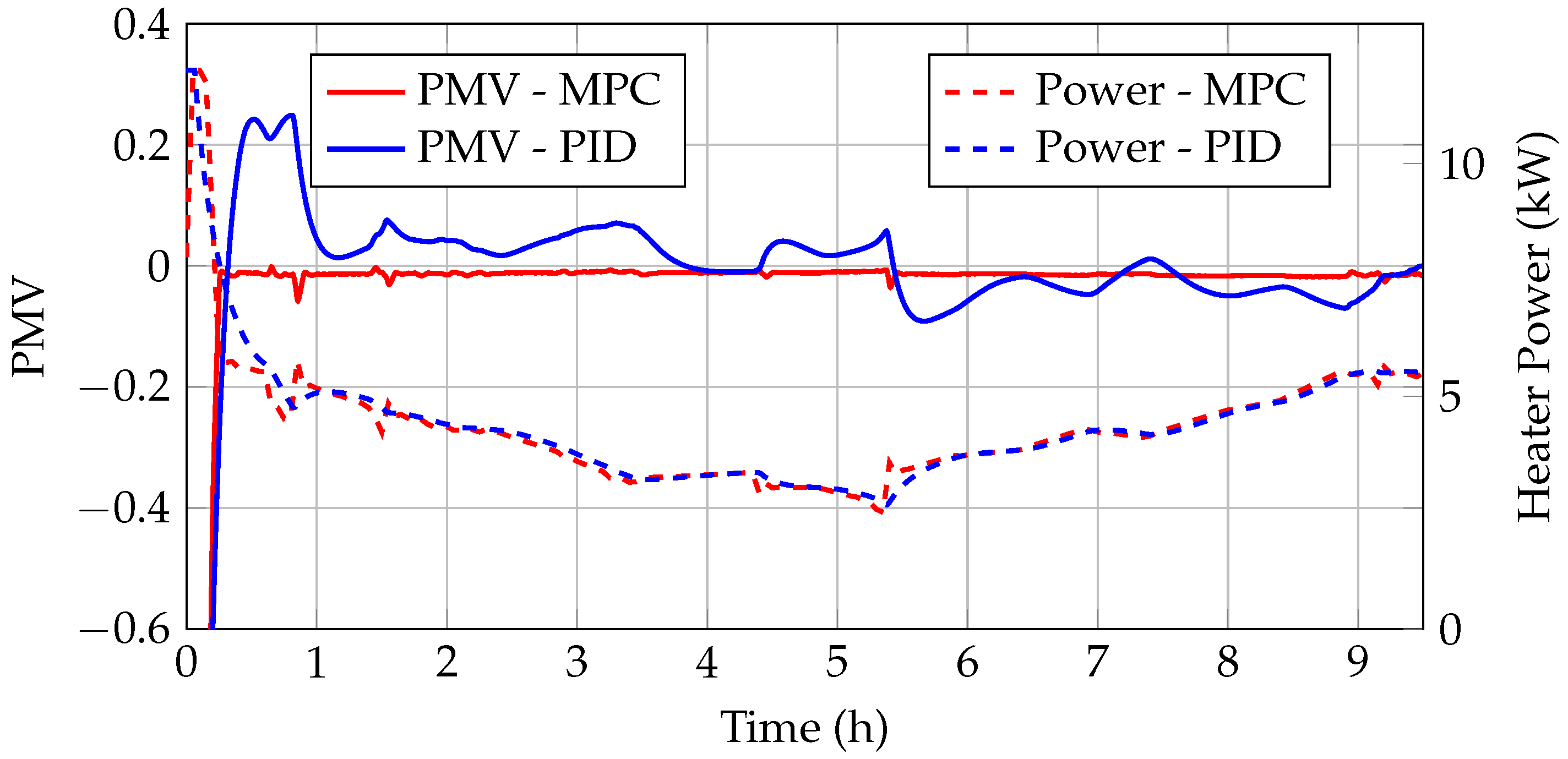
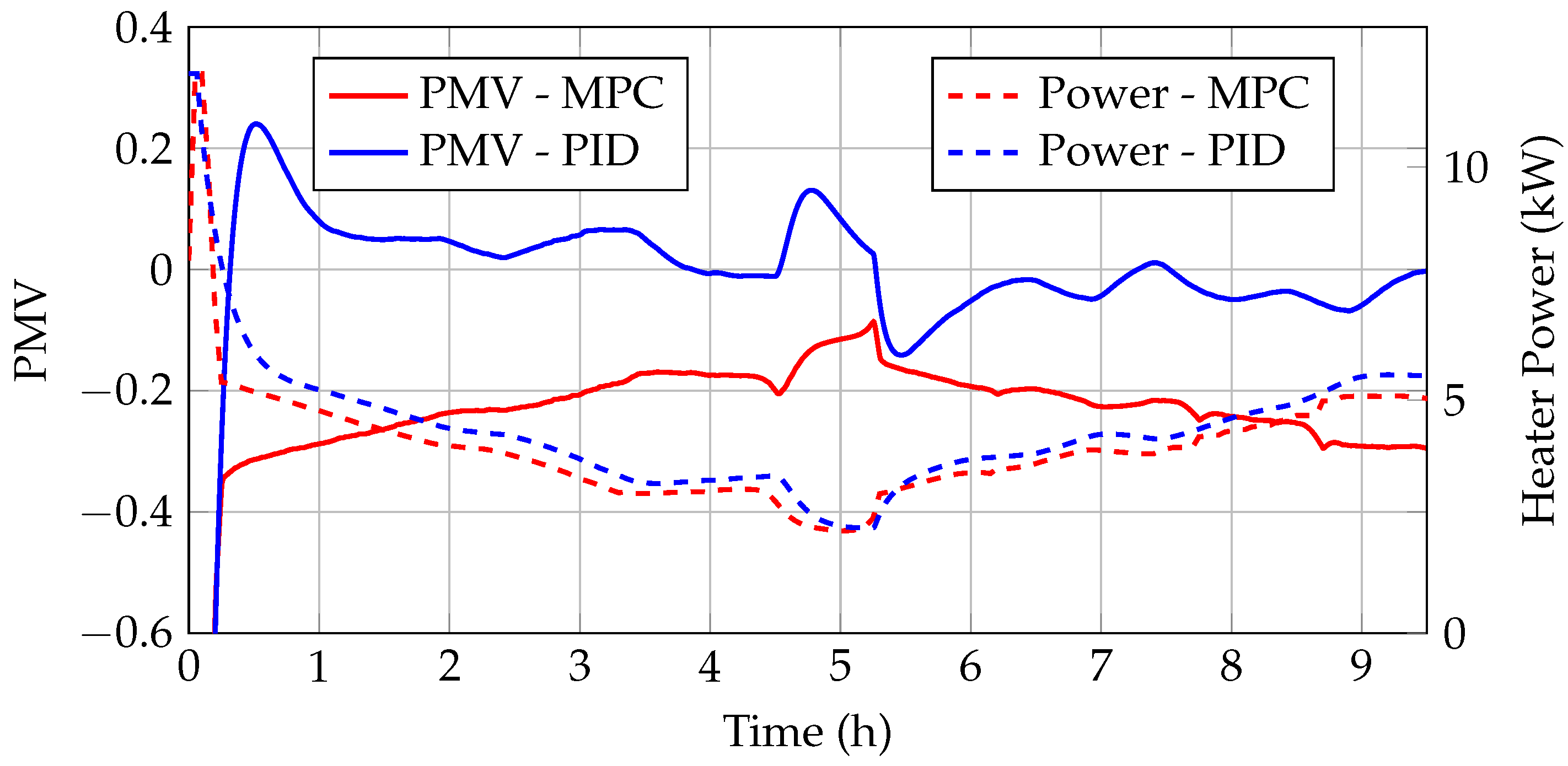
As explained in Section 4.1.1, an average winter day with temperatures ranging from 0 to 8 °C was selected to represent typical winter conditions for the truck. The simulation results are shown in Figure 19, with both controllers using a target PMV value of 0.

Comparing both controllers using $\mathrm{PMV}=0$ as the reference value highlights the challenges faced by the PID controller in handling nonlinear systems and external disturbances. Although the PID gains were previously tuned in Simulink, significant deviations from the set PMV value are visible. In contrast, the MPC demonstrates stability and robustness, performing better due to its predictive capabilities. By anticipating and adapting to dynamic changes in the system, MPC maintains consistent performance with negligible fluctuations in the PMV value. By eliminating the initial overshoot seen with PID and maintaining a more stable heating power, MPC achieves a 0.5% reduction in energy consumption.

While MPC can maintain a near-constant PMV, the purpose of this study is to achieve the acceptable thermal comfort range and, once inside, balance thermal comfort with energy demand to reduce overall consumption. This strategy allows for energy savings while maintaining an acceptable average PMV. Different weighting factor configurations for MPC were tested, with the resulting average PMV values and energy consumption summarized in

Table 8. MPC and PID energy consumption for average winter day and SeLv cycle.

Controller	${\mathit{PMV}}_{\mathit{avg}}$	Energy Consumption [kWh]	Comparison
PID	0	$48.68$	-
PID	$-0.2$	$45.66$	$-\mathrm{6.2\%}$
MPC	$-0.2$	$45.54$	$-\mathrm{6.9\%}$

. As expected, a slightly lower average PMV corresponds to reduced energy consumption.

In Figure 20, the PMV values achieved using MPC are compared with those from the PID controller for the SeLv velocity profile and average winter conditions. The corresponding energy savings relative to the PID controller are presented in Table 8. For a fair comparison, an additional simulation was run in which the PID controller was given the average PMV value achieved by MPC as its target. The results highlight the difference in control strategies: while the PID maintains a fixed PMV reference, the MPC dynamically adjusts the average PMV in response to operating conditions, optimizing the trade-off between thermal comfort and energy efficiency.

Under average SeLv operating conditions, the MPC strategy demonstrates strong potential for reducing heating system energy consumption. Over a 9.5 h drive, it achieves a 6.9% reduction in energy usage while maintaining an average PMV of −0.2, well within the acceptable thermal comfort range. Compared to the conventional PID controller with a fixed reference, MPC not only reduces energy consumption by an additional 0.7% but also maintains a notably more stable PMV, further enhancing occupant comfort consistency.

4.3.2. Average Winter Day with VECTO Velocity Profile

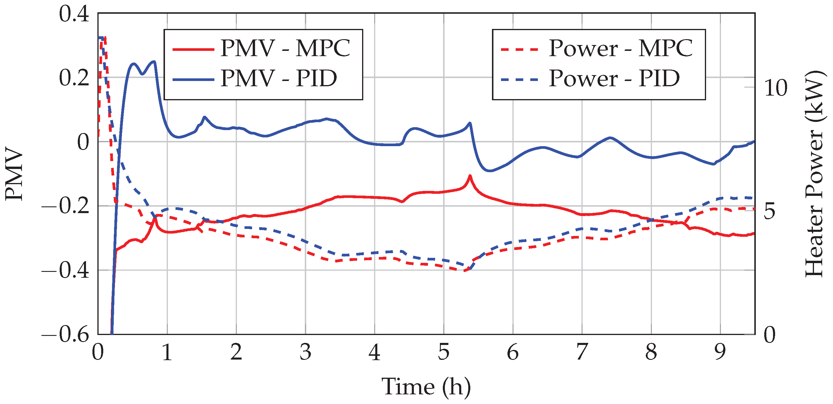
For the same ambient conditions, the controller is next evaluated using the VECTO driving cycle. This cycle was selected due to its frequent velocity changes, which allow assessment of the impact of varying driving conditions on control stability. The PMV values obtained from the MPC and PID simulations are plotted in Figure 21, and the corresponding performance comparison is presented in

Table 9. MPC and PID energy consumption for average winter day and VECTO cycle.

Controller	${\mathit{PMV}}_{\mathit{avg}}$	Energy Consumption [kWh]	Comparison
PID	0	$54.76$	-
MPC	$-0.22$	$50.33$	−8.1%

.

The effect of the changed velocity profile is evident for the PID controller, which exhibits larger fluctuations in PMV values when operating under conditions different from its tuning environment. In contrast, the MPC maintains a much smoother PMV evolution, achieving levels comparable to those seen in Figure 20, while also preserving a similar reduction in energy consumption. This comparison highlights the superior performance of MPC over PID control when exposed to driving conditions different from the tuning scenario.

4.3.3. Cold Winter Day with SeLv Velocity Profile

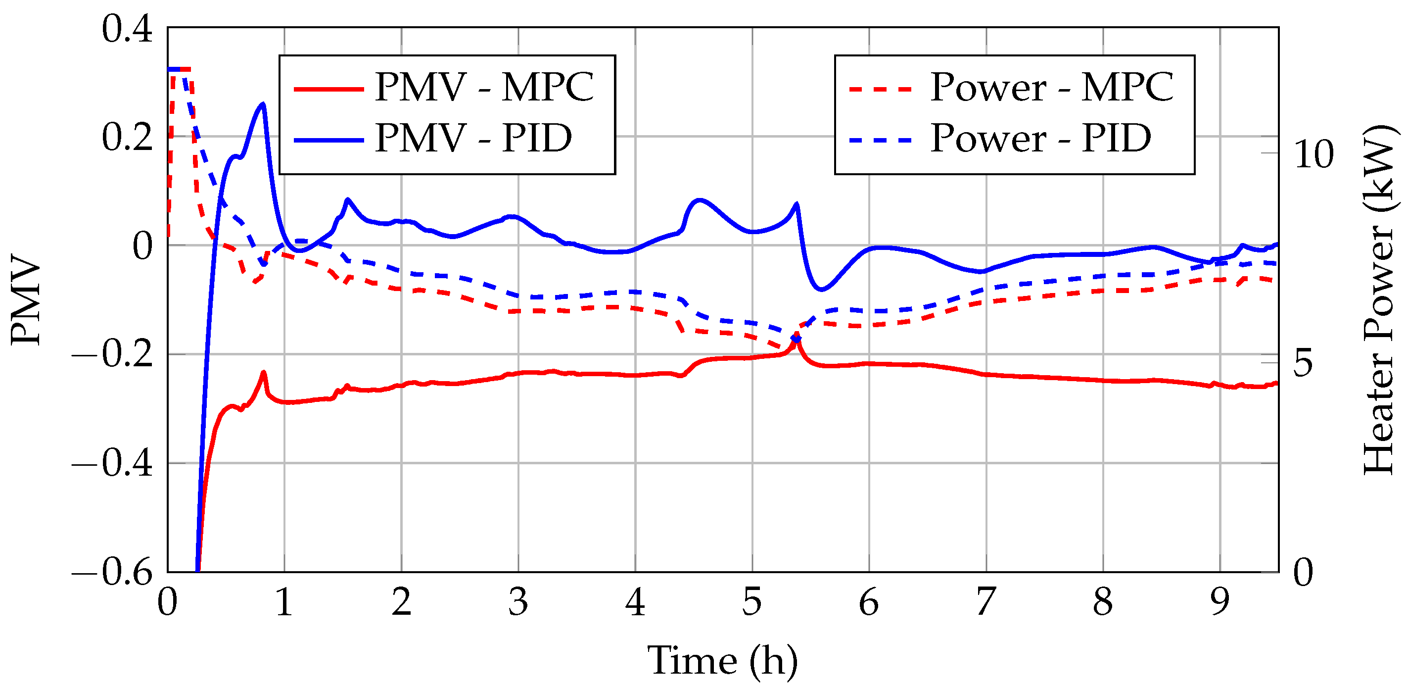
Next, the SeLv velocity profile was simulated for ambient conditions corresponding to a cold winter day in Aachen, as shown in Figure 15. Initial simulations using the weighting factors from the average winter day resulted in larger deviations from the ideal PMV values. Consequently, a new set of weighting factors was adapted for these colder conditions. The behavior of both controllers under the SeLv driving cycle is shown in Figure 22, and the comparison of PID and MPC performance is summarized in

Table 10. MPC and PID energy consumption for a cold winter day with the SeLv cycle using updated weighting factors.

Controller	${\mathit{PMV}}_{\mathit{avg}}$	Energy Consumption [kWh]	Comparison
PID	0	$63.08$	-
MPC	$-0.2$	$60.53$	$-4\%$

.

4.3.4. Cold Winter Day with the VECTO Velocity Profile

Simulations using the VECTO urban delivery cycle under cold ambient conditions were conducted with the updated weighting factors described in the previous section. The evolution of the PMV values for both controllers is shown in Figure 23, and the corresponding performance metrics are summarized in

Table 11. MPC and PID energy consumption for cold winter day and VECTO cycle with updated weighting factors.

Controller	${\mathit{PMV}}_{\mathit{avg}}$	Energy Consumption [kWh]	Comparison
PID	0	$67.75$	-
MPC	$-0.24$	64	$-5.5\%$

.

4.3.5. Coupling with Cooling Circuit

The objective of this investigation is to assess the potential energy savings in the heating system when it is coupled with the medium-temperature (MT) cooling circuit and to evaluate the MPC’s capability in managing multi-input, multi-output (MIMO) systems. To accommodate the dynamic changes in coolant system parameters following valve activation, the MPC configuration has been adjusted accordingly. A step size of 10 s was chosen, with prediction and control horizons set to 8 and 4, respectively.

The state functions were updated to incorporate the newly derived algebraic expression for the coolant temperature entering the HV heater (see Equation (34)), where $w_{valve}$ is defined as a manipulated variable (MV), and $T_{waste}$ is assigned a constant value of 40 °C. The cost function structure remains unchanged, ensuring that the MPC continues to regulate both heating power and valve position to maintain a balance between thermal comfort and energy efficiency comparable to the performance observed previously.

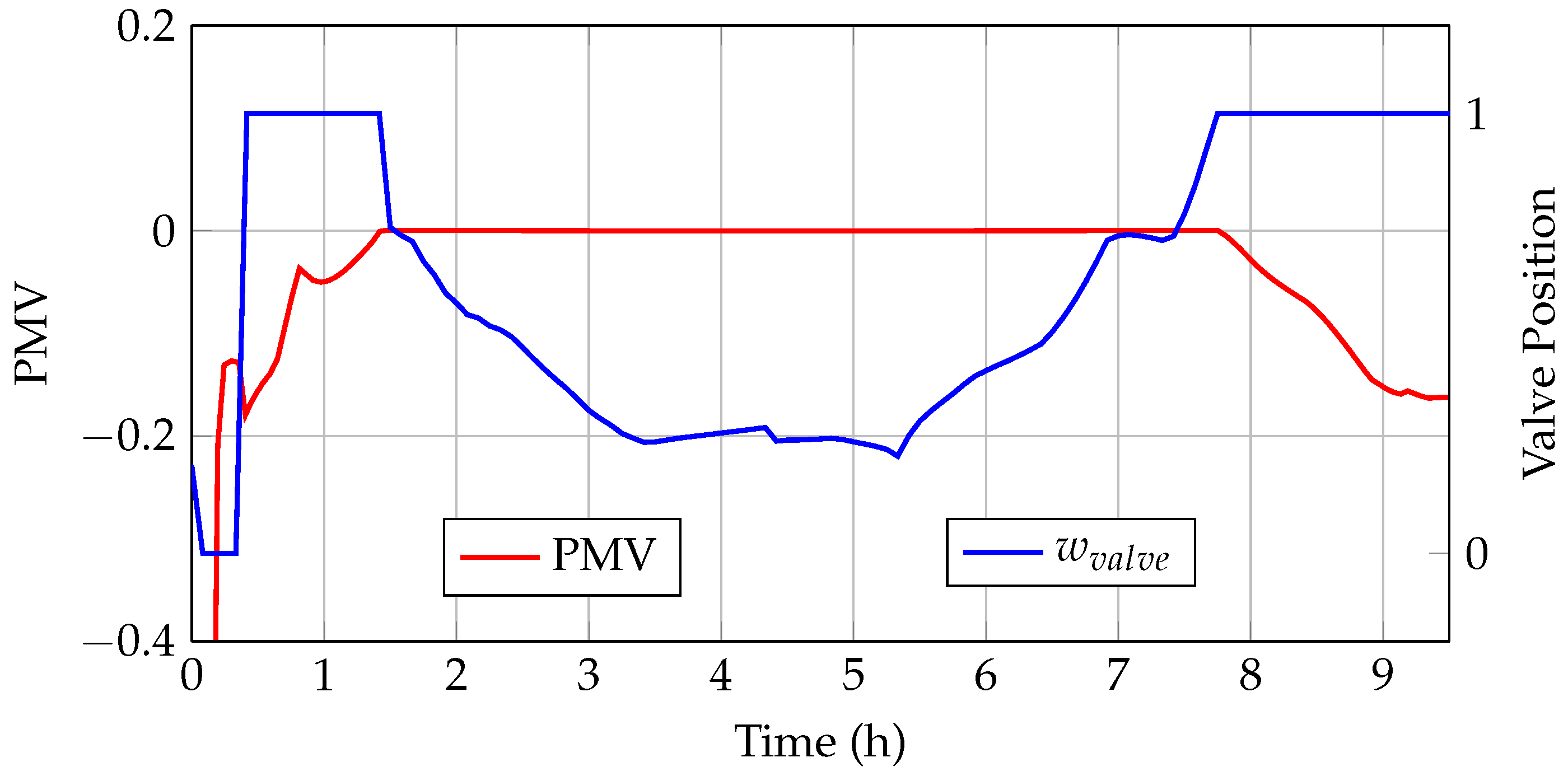
The system performance is illustrated in Figure 24, based on a simulation conducted under extreme cold conditions with the SeLv velocity profile. Initially, the MPC prioritizes bringing the cabin into the acceptable thermal comfort region as quickly as possible, keeping the valve closed to maximize the coolant temperature. Once the cabin stabilizes within the comfort region, the MPC opens the valve, allowing the waste heat from the drivetrain cooling system to be utilized, thereby reducing the energy consumption of the HV heater. Toward the end of the simulation, as ambient temperature decreases, the MPC encounters greater difficulty in maintaining thermal comfort and responds by closing the valve to increase the coolant temperature.

To provide an overview of the potential energy savings achieved by utilizing drivetrain waste heat for cabin heating, the results of the two simulations are summarized in

Table 12. MPC and PID energy consumption for cold winter day and SeLv cycle with coupled cooling system.

Controller	${\mathit{PMV}}_{\mathit{avg}}$	Energy Consumption [kWh]	Comparison
PID	$-0.2$	$63.86$	-
MPC	$-0.193$	50	$-21.7\%$

. Defining an optimal control strategy for the valve is particularly challenging in this coupling scenario. If the outlet temperature from the cabin heat exchanger exceeds the temperature in the MT cooling circuit, mixing the coolant would be counterproductive and could increase energy consumption. Here, the advantage of the MPC becomes evident: the controller autonomously recognizes when the valve should be closed, as the energy consumption is accounted for in the cost function.

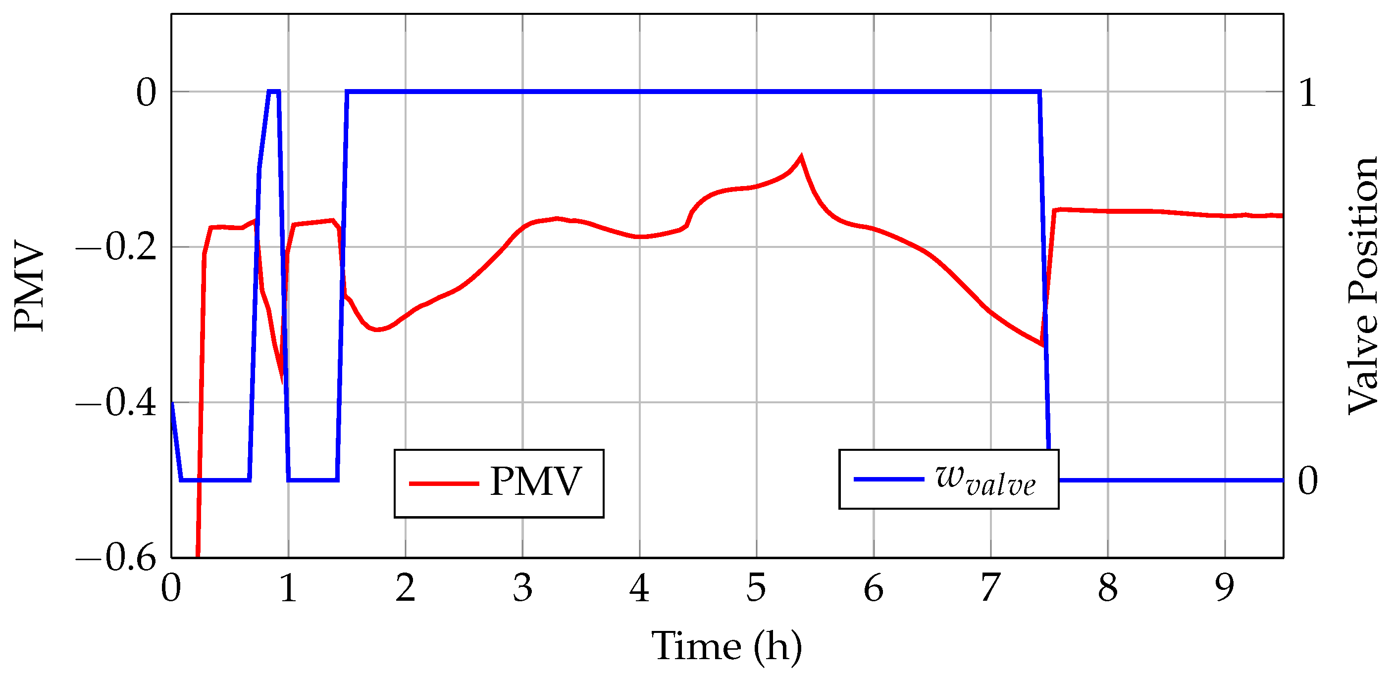
The simulation was repeated using the average winter temperature profile together with the SeLv velocity profile. The resulting PMV and valve position ($w_{valve}$) are shown in Figure 25. In this scenario, due to the higher ambient temperatures, the waste heat from the drivetrain cooling system was sufficient to maintain a stable cabin temperature and a PMV value close to 0 once the acceptable thermal comfort region was reached. Consequently, the MPC turned off the heater and regulated the PMV solely through adjustments of the valve position. Toward the end of the simulation, as ambient temperature decreased, the MPC reactivated the heater to maintain thermal comfort.

5. Discussion

This paper highlights the advantages of MPC compared to traditional control strategies in the context of cabin heating for heavy-duty trucks. As vehicle electrification advances, thermal management systems become increasingly complex. Although this complexity presents new challenges for optimal control, it also introduces greater flexibility in thermal energy distribution. Efficient control strategies, therefore, play a crucial role in ensuring energy-efficient and reliable thermal management.

The analysis of results, particularly in Figure 19, demonstrates that MPC outperforms traditional control methods in maintaining cabin thermal comfort. This improvement is primarily attributed to MPC’s ability to anticipate and compensate for external disturbances through its predictive capabilities. However, a direct comparison between MPC when simply maintaining thermal comfort and traditional control shows only moderate energy savings. The real strength of MPC lies in its flexibility to incorporate optimization objectives. By formulating a cost function that explicitly balances thermal comfort and energy consumption, MPC can significantly improve overall system efficiency. This was demonstrated in further examples with different ambient conditions and driving cycle, where the average PMV value was slightly lower than the set value of 0 but still in the acceptable range, yet significant energy savings were achieved.

While similar energy-saving outcomes may be achievable with conventional PID controllers by dynamically adjusting the target PMV value, this approach introduces additional complexity. PID controllers require predefined setpoint schedules, typically determined through extensive calibration using look-up tables or offline optimization. Both methods are either time-consuming or computationally demanding. In contrast, MPC integrates optimization directly into the control process, enabling real-time trade-offs between competing objectives. Although this increases computational requirements, it centralizes decision-making and removes the need for manual tuning or extensive calibration.

The most notable performance of MPC was demonstrated in the case study involving its coupling with the medium-temperature cooling circuit via a three-way valve, as discussed in Section 4.3.5. This example effectively illustrates the strength of MPC in managing MIMO systems. By formulating an appropriate cost function, MPC was able to determine an optimal control strategy for the three-way valve that simultaneously accounted for heating demand and cabin thermal comfort.

A key advantage of MPC in this context is its ability to inherently consider energy efficiency within its optimization. For instance, the controller avoids coupling the cabin heating circuit with the MT cooling loop when the MT temperature is lower than the outlet temperature of the cabin heat exchanger, an operation that would be energetically counterproductive. While a similar coupling strategy could theoretically be achieved using rule-based control, doing so would require significantly more complex logic to prevent inefficient operating conditions, as previously discussed. In contrast, MPC simplifies the development process by embedding this decision-making logic within its optimization framework, reducing the need for extensive manual tuning or heuristic rule design. As a result, MPC not only improves control performance but also reduces development effort when integrating complex subsystem interactions. Nevertheless, practical implementation could face additional challenges not captured in the simulation. For instance, the dynamics of the three-way valve are not considered in the current model. In practice, the valve requires approximately $5\mathrm{s}$ to move from fully closed to fully open and its position is controlled in discrete steps (0–90°) with a resolution of 1°. These factors could introduce delays or precision limitations when coupling the cabin heating system with the MT cooling circuit, which may slightly degrade real-world control performance compared to simulation results.

While this study focused on cabin heating, similar advantages of MPC can be expected for cabin cooling. In cooling mode, predictive control could anticipate solar radiation loads and ambient temperature changes, allowing proactive adjustment of compressor operation, airflow distribution, and chilled coolant temperature. Cooling also introduces additional complexity due to competition for thermal resources with other subsystems, such as battery or fuel cell cooling loops. Here, the MIMO capabilities of MPC would be particularly beneficial, enabling the controller to balance passenger comfort against overall vehicle thermal efficiency. By integrating solar irradiance forecasts and predicted driving conditions into the optimization, MPC could reduce compressor energy consumption while maintaining acceptable comfort levels, potentially achieving even greater relative energy savings than in heating scenarios. Exploring these aspects offers a promising direction for future work.

In conclusion, MPC provides a powerful and flexible approach for controlling advanced thermal management systems in electrified trucks, especially when both thermal comfort and energy efficiency must be simultaneously considered. This study contributes further by (i) presenting an MPC-based approach to the cabin heating system of heavy-duty fuel cell trucks, (ii) quantifying efficiency gains and comfort improvements over conventional controllers, and (iii) analyzing the integration with the medium-temperature cooling circuit. These findings highlight the potential of predictive control methods to enable more energy-efficient and reliable thermal management strategies for next-generation fuel cell trucks.

References

1. Kraftfahrt-Bundesamt. Fahrzeugzulassungen (FZ): Bestand an Kraftfahrzeugen und Kraftfahrzeuganhängern nach Zulassungsbezirken. Available online: https://www.kba.de/DE/Statistik/Fahrzeuge/Bestand/ZulassungsbezirkeGemeinden/zulassungsbezirke_node.html?yearFilter=2022 (accessed on 31 May 2025).
2. Bundesministerium für Digitales und Verkehr. Verkehr in Zahlen 2024/2025. Available online: https://www.bmv.de/SharedDocs/DE/Anlage/G/verkehr-in-zahlen24-25-pdf.pdf?__blob=publicationFile (accessed on 31 May 2025).
3. Umweltbundesamt. Daten der Treibhausgasemissionen des Jahres 2022 nach KSG. Available online: https://www.umweltbundesamt.de/themen/klima-energie/treibhausgas-emissionen (accessed on 31 May 2025).
4. Verband der Automobilindustrie (VDA). Tatsachen und Zahlen 2022; VDA: Berlin, Germany, 2022. [Google Scholar]
5. O’Connell, A.; Pavlenko, N.; Bieker, G.; Searle, S. A Comparison of the Life-Cycle Greenhouse Gas Emissions of European Heavy-Duty Vehicles and Fuels. Available online: https://theicct.org/publication/lca-ghg-emissions-hdv-fuels-europe-feb23/ (accessed on 18 March 2025).
6. Schwere Lastkraftwagen für die Emissionsfreie Logistik im Schwerlastverkehr Mittels Elektrifizierungsbaukasten und Wirtschaftlichem Produktionssystem. Available online: https://selv.rwth-aachen.de/ (accessed on 31 May 2025).
7. Heimes, H.H.; Kampker, A.; Kehrer, M.; Hagedorn, S.; Biegler, S.; Hausmann, J. Strategien zur Erreichung der Emissionsziele im Nutzfahrzeugsektor. Available online: https://www.pem.rwth-aachen.de/global/show_document.asp?id=aaaaaaaabvnrmmf (accessed on 18 March 2025).
8. Chong, H.; Rightor, E. Closing the Trucking Gaps: Priorities for the Department of Energy’s RD&D Portfolio. Available online: https://itif.org/publications/2023/06/20/closing-the-trucking-gaps-priorities-for-the-department-of-energys-rd-and-d-portfolio (accessed on 18 March 2025).
9. Draz, U.; Bartolomeo, E.D.; Panunzi, A.P.; Laverdura, U.P.; Lisi, N.; Chierchia, R.; Duranti, L. Copper-Enhanced CO2 Electroreduction in SOECs. CS Appl. Mater. Interfaces 2024, 16, 8842–8852. [Google Scholar] [CrossRef] [PubMed]
10. e-mobil BW GmbH; AVL; ZSW. Systemvergleich Zwischen Wasserstoff-Verbrennungsmotor und Brennstoffzelle im Schweren Nutzfahrzeug. Available online: https://www.e-mobilbw.de/fileadmin/media/e-mobilbw/Publikationen/Studien/e-mobilBW-Studie_H2-Systemvergleich.pdf (accessed on 31 May 2025).
11. Arminger, G.; Bonne, T. Einfluss der Witterung auf das Unfallgeschehen im Strassenverkehr. ATZ—Automob. Z. 1999, 101, 675–678. [Google Scholar] [CrossRef]
12. Alizadeh, M.; Dhale, S.; Emadi, A. A Critical Review and Future Prospects of Control-Oriented HVAC Modeling Strategies in Electric Vehicles. IEEE Trans. Transp. Electrif. 2014, 72, 343–355. [Google Scholar] [CrossRef]
13. Proportional, Integral, Derivative (PID) Control for HVAC. Available online: https://www.eaton.com/us/en-us/products/controls-drives-automation-sensors/industrial-control-center/automation-control/hvac-control/pid-control.html (accessed on 18 March 2025).
14. Daly, S. Automotive Air Conditioning and Climate Control Systems, 1st ed.; Elsevier Ltd.: Burlington, VT, USA, 2006; p. 169. [Google Scholar]
15. Kasahara, M.; Matsuba, T.; Kuzuu, Y.; Yamazaki, T.; Hashimoto, Y.; Kamimura, K.; Kurosu, S. Design and tuning of robust PID controller for HVAC systems. In ASHRAE Transactions 105; ASHRAE: Seattle, WA, USA, 1999. [Google Scholar]
16. Liu, Z.; Xu, S.; Zhang, B.; Guo, S. Voltage tracking and regulation of vehicle PEMFC system under low load condition based on fuzzy LQG hybrid strategy. ISA Trans. 2025, 165, 510–523. [Google Scholar] [CrossRef] [PubMed]
17. Afram, A.; Janabi-Sharifi, F. Theory and applications of HVAC control systems—A review of model predictive control (MPC). Build. Environ. 2014, 72, 343–355. [Google Scholar] [CrossRef]
18. Xie, Y.; Liu, Z.; Li, K.; Liu, J.; Zhang, Y.; Dan, D.; Wu, C.; Wang, P.; Wang, X. An improved intelligent model predictive controller for cooling system of electric vehicle. Appl. Therm. Eng. 2021, 182, 116084. [Google Scholar] [CrossRef]
19. Schwenzer, M.; Ay, M.; Bergs, T.; Abel, D. Review on model predictive control: An engineering perspective. Int. J. Adv. Manuf. Technol. 2021, 117, 1327–1349. [Google Scholar] [CrossRef]
20. Rajasingham, T.A. Nonlinear Model Predictive Control of Combustion Engines, 3rd ed.; Springer Nature: Cham, Switzerland, 2021; pp. 154–196. [Google Scholar]
21. Kampker, A.; Heimes, H.H.; Schmitt, F.; Hadzovic, T.; Betz, M. Simulation-Based Development of Thermal Management for Heavy Duty Fuel Cell Commercial Vehicles. In Proceedings of the 23rd Internationales Stuttgarter Symposium, Stuttgart, Germany, 4–5 July 2023. [Google Scholar]
22. Simulink—MATLAB & Simulink. Available online: https://de.mathworks.com/products/simulink.html (accessed on 15 July 2025).
23. Lienhard, J.H., IV; Lienhard, J.H., V. A Heat Transfer Handbook, 5th ed.; Phlogiston Press: Cambridge, MA, USA, 2020; pp. 120–127. [Google Scholar]
24. Incropera, F.P.; Dewitt, D.P.; Bergman, T.L.; Lavine, A.S. Fundamentals of Heat and Mass Transfer, 6th ed.; John Wiley & Sons: Hoboken, NJ, USA, 2007; p. 689. [Google Scholar]
25. Simcenter Amesim Software. Available online: https://plm.sw.siemens.com/en-US/simcenter/systems-simulation/amesim/ (accessed on 15 July 2025).
26. Spitler, J.D. Load Calculation Applications Manual; ASHRAE: Atlanta, GA, USA, 2014. [Google Scholar]
27. Favoino, F.; Raheli, E.; Ramirez, D.; Pilosio, F.; Tavarnese, S.; Simonetti, M.; Perino, M.; Masoero, M. Impact of glass technology on future electrical individual transportation: The Pop.Up case study. Glass Struct. Eng. 2020, 5, 117–131. [Google Scholar] [CrossRef]
28. ISO/DIS 7730; Ergonomics of the Thermal Environment. Analytical Determination and Interpretation of Thermal Comfort Using Calculation of the PMV and PPD Indices and Local Thermal Comfort Criteria. International Organization for Standardization: Geneva, Switzerland, 2023.
29. Fanger, P.O. Thermal Comfort: Analysis and Applications in Environmental Engineering; Danish Technical Press: Copenhagen, Denmark, 1970; Available online: https://api.semanticscholar.org/CorpusID:110028033 (accessed on 7 July 2025).
30. Fayazbakhsh, M.A.; Bahrami, M. Comprehensive Modeling of Vehicle Air Conditioning Loads Using Heat Balance Method. SAE Tech. Pap. 2013, 1, 1507. [Google Scholar]
31. Zhang, Y.; Li, Z.; Liu, S.; Wang, G.; Chang, H. A Study of Passenger Car Cabin Pre-Ventilation under the Sun. Energies 2023, 16, 7154. [Google Scholar] [CrossRef]
32. Wang, H.; Kolmanovsky, I.; Amini, M.R.; Sung, J. Model Predictive Climate Control of Connected and Automated Vehicles for Improved Energy Efficiency. In Proceedings of the 2018 American Control Conference, Milwaukee, WI, USA, 27–29 June 2018. [Google Scholar]
33. Liou, K.N. An Introduction to Atmospheric Radiation, 2nd ed.; Academic Press: San Diego, CA, USA, 2002. [Google Scholar]
34. Weng, M.; Zhang, Y.; Liu, F.; Liu, A.; Zhang, H. Optimization of airflow organization in the passenger cabin of special vehicles based on human thermal sensation. Case Stud. Therm. Eng. 2025, 65, 105678. [Google Scholar] [CrossRef]
35. ANSI/ASHRAE Standard 55-2010; Thermal Environmental Conditions for Human Occupancy. American Society of Heating, Refrigerating and Air-Conditioning Engineers: Atlanta, GA, USA, 2010.
36. Tetens, V.O. Über einige meteorologische Begriffe. Z. Geophys. 1930, 6, 297–309. [Google Scholar]
37. Portables System—BRIXX. Available online: https://www.gantner-instruments.com/de/produkte/brixx/ (accessed on 10 August 2025).
38. ISO/DIS 7726; Ergonomics of the Thermal Environment. Instruments for Measuring and Monitoring Physical Quantities. International Organization for Standardization: Geneva, Switzerland, 2023.
39. Kampker, A.; Heimes, H.H.; Schmitt, F.; Backes, T.; Betz, M.; Hadzovic, T. Design of an Electric Drive Axle for Heavy Duty Commercial Vehicles in the Long-Haul Application Under Consideration of Energy Consumption. In Proceedings of the 12th International Electric Drives Production Conference (EDPC) 2022, Regensburg, Germany, 29–30 November 2022. [Google Scholar]
40. Vehicle Energy Consumption Calculation TOol—VECTO. Available online: https://climate.ec.europa.eu/eu-action/transport-decarbonisation/road-transport/vehicle-energy-consumption-calculation-tool-vecto_en (accessed on 1 June 2025).
Figure 1. Overview of the motivation to electrify heavy-duty vehicles: (a) Vehicle distribution in Germany in 2022, where heavy-duty trucks constitute only 1%. (b) CO2 emissions according to sector in Germany in 2022. (c) Distribution of CO2 emissions within mobility sector. (d) Trend of growth in goods transport.
Wevj 16 00568 g001
Figure 2. Model predictive control working principle. Adapted from [19].
Wevj 16 00568 g002
Figure 3. Heating system layout of the SeLv truck.
Wevj 16 00568 g003
Figure 4. Experimentally determined relationship between coolant volume flow and temperature.
Wevj 16 00568 g004
Figure 5. Heat loads acting on the cabin [27].
Wevj 16 00568 g005
Figure 6. PPD as a function of PMV. The shaded area shows the comfortable region with PPD < 10%.
Wevj 16 00568 g006
Figure 7. Overview of the sensor positioning in the driver cabin.
Wevj 16 00568 g007
Figure 8. PMV measurement stand used inside the cabin: (a) upper part for torso and head measurements, and (b) lower part for ankle-level measurements.
Wevj 16 00568 g008
Figure 9. Comparison of measured and simulated relative humidity.
Wevj 16 00568 g009
Figure 10. Mean radiant temperature measurements: (a) Comparison of mean radiant temperature at head level with air and wall temperature measurements. (b) Mean radiant temperature measurements at different heights.
Wevj 16 00568 g010
Figure 11. Validation of simulated and measured coolant inlet and outlet temperatures in the heating system.
Wevj 16 00568 g011
Figure 12. Comparison of measured and simulated air temperature at the heat exchanger outlet (air entering the cabin).
Wevj 16 00568 g012
Figure 13. Measured and simulated temperatures used to validate the external heat load calculation.
Wevj 16 00568 g013
Figure 14. Measured and simulated temperatures used to validate the model including solar irradiance effects.
Wevj 16 00568 g014
Figure 15. Ambient temperature profiles used as input for the simulations.
Wevj 16 00568 g015
Figure 16. SeLv driving cycle.
Wevj 16 00568 g016
Figure 17. VECTO urban delivery cycle.
Wevj 16 00568 g017
Figure 18. Illustration of the MPC strategy balancing thermal comfort and energy consumption.
Wevj 16 00568 g018
Figure 19. Comparison of MPC and PID performance for an average winter day with the SeLv velocity profile.
Wevj 16 00568 g019
Figure 20. MPC and PID achieved PMV for an average winter day with the SeLv cycle.
Wevj 16 00568 g020
Figure 21. MPC and PID achieved PMV for an average winter day with the VECTO cycle.
Wevj 16 00568 g021
Figure 22. MPC and PID achieved PMV for a cold winter day with the SeLv cycle using updated weighting factors.
Wevj 16 00568 g022
Figure 23. MPC and PID achieved PMV for a cold winter day with the VECTO cycle using updated weighting factors.
Wevj 16 00568 g023
Figure 24. PMV and valve position for a cold winter day with the SeLv cycle and coupled cooling system.
Wevj 16 00568 g024
Figure 25. PMV and valve position for average winter day and SeLv cycle with coupled cooling system.
Wevj 16 00568 g025