Article

An Enhanced State-Space Modeling for Detecting Abnormal Aging in VRLA Batteries

by
Humberto Velasco-Arellano
,
Nancy Visairo-Cruz
*,
Ciro Alberto Núñez-Gutiérrez
and
Juan Segundo-Ramírez
Facultad de Ingeniería, Universidad Autonoma de San Luis Potosí, San Luis Potosí 78300, Mexico
*
Author to whom correspondence should be addressed.
World Electr. Veh. J. 2024, 15(11), 507; https://doi.org/10.3390/wevj15110507
Submission received: 11 October 2024 / Revised: 27 October 2024 / Accepted: 1 November 2024 / Published: 5 November 2024
(This article belongs to the Topic Battery Design and Management)

Abstract

:
The knowledge of battery aging is an indicator that allows controlling the performance of large battery banks. State of Health (SOH) is typically the metric used, encompassing all possible mechanisms in a percentage indicator, with the Coulomb Counting as the most common method. Hence, an in-depth study of aging based on known models provides proper information for correctly managing batteries. This article proposes an aging-sensitive 3-RC-array-equivalent electrical circuit model to characterize the behavior of batteries throughout their useful life, identifying parametric changes as complementary information to the state of health. This model was validated based on experimental tests with 2 V and 6 Ah VRLA batteries aged according to the manufacturer’s recommended use. The results reveal a proportionality through capacity degradation. Then, a control group of batteries was subjected to overcharge and over-discharge conditions. The information given by Coulomb Counting SOH and the proposed method were evaluated. The proposed method provides additional information to the SOH, enhancing the distinguishing capability between typical aging performance and misused aging performance, resulting in a useful tool capable of identifying the aging associated with parametric changes in a time-invariant system where aging is treated as an imminent multiplicative fault.

1. Introduction

In the modern world, dominated by technology whose impulse is electrical energy, energy storage is a big concern for many companies and customers. Several demanding applications require energy storage backup as a central component of the process, such as electric vehicles [1,2], energy-distributed resources [3,4], and Uninterruptible Power Supply (UPS) for the critical process [5,6], to name a few. A usual method of storing energy is using batteries because they are suitable for being constructed in many technologies, energy densities, weights, volumes, and other electric characteristics [7]. Valve-regulated lead-acid (VRLA) batteries are among the most popular [8,9]. In terms of production, maintenance, and recycling, VRLA batteries are competitive [10]. Another advantage is their relative stability to external variables and maintaining commercial usage [11].
The batteries provide the system with flexibility, but if they fail, the operation of the system shall be compromised and even stopped. Therefore, challenges are emerging, such as better materials for construction [12], battery power delivery [13], battery storage management [14], and fault detection [15]. One of the ways to address these problems is through mathematical modeling of batteries, which should faithfully represent the behavior of the battery throughout its lifetime [16,17]. The equivalent electrical circuit model is one aspect of modeling applied to batteries because of its simplicity and ability to represent the cells’ critical internal states [7]. It is widely recognized that the Equivalent Electric Circuit (EEC) model of a battery is impacted by the SOH changes throughout the battery’s lifetime [18]. Therefore, investigating the battery’s aging mechanisms and how they affect the EEC parameters [13] can provide valuable evidence of fault conditions, especially if the degradation process occurs in an atypical form [19].
In the state-of-the-art, there are several methodologies for estimating the SOH indirectly; Table 1 lists some of them.
An analysis of the state-of-the-art is summarized in Table 1 and considers the advantages of each methodology. However, in all cases, the SOH estimation method is refined, improving its performance under different conditions but maintaining the quality of being a single percentage that encompasses a multifactorial phenomenon.
In this research, a nonlinear state-space model of the EEC capable of distinguishing between normal aging and misused aging conditions is proposed. For purposes of validation, an experimental battery setup was used for estimating the parametric variations along the lifetime of the battery, including overcharge and over-discharge cases. The findings permit the establishment of multiplicative faults affecting the parameters. If those faults appear at an atypical battery age, the model can help to detect imminent or direct faults only using voltage and current measurements, unlike the methods given in Table 1 that only improve the SOH estimation. Although VRLA batteries are the focus of this paper, the methodology can be applied to any redox battery technology.
The article is organized as follows. In Section 2, system modeling and the nonlinear observer are developed. Section 3 describes the experiment setup for validation and describes the tendencies in normal conditions. Section 4 describes the overcharge and over-discharge test cases to evaluate the operating limits of the methodology. Section 5 provides a conclusion of the contributions of this work.

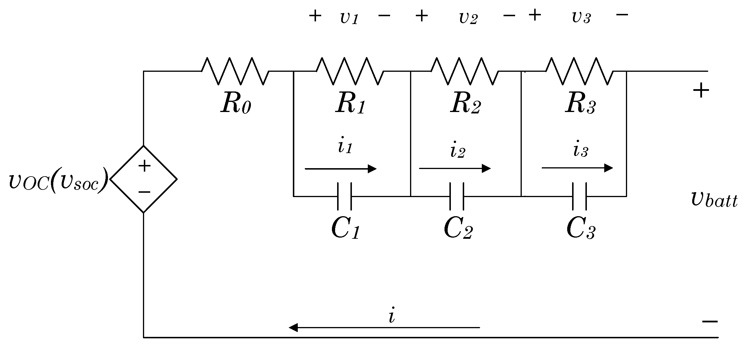
2. Battery Equivalent Circuit Model
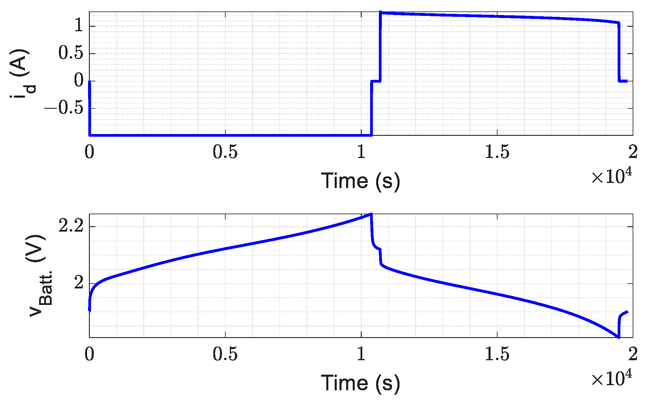
An approximation to an EEC model of the battery is used for practical purposes, analogically defining the electrochemical phenomena with known electrical elements that closely coincide with the observed behavior [29].
The EEC model used is shown in Figure 1 [30], which consists of an open circuit voltage v O C that is SOC-dependent and therefore should be estimated online [15], a resistance R 0 followed by three R C tanks [29], an output voltage v b a t t , and an input current (i).
The model can be put together as follows:
  • Measurable variables: the voltage ( v b a t t ) is the model output, and the current (i) is the model input [7]; the temperature is considered constant for this work.
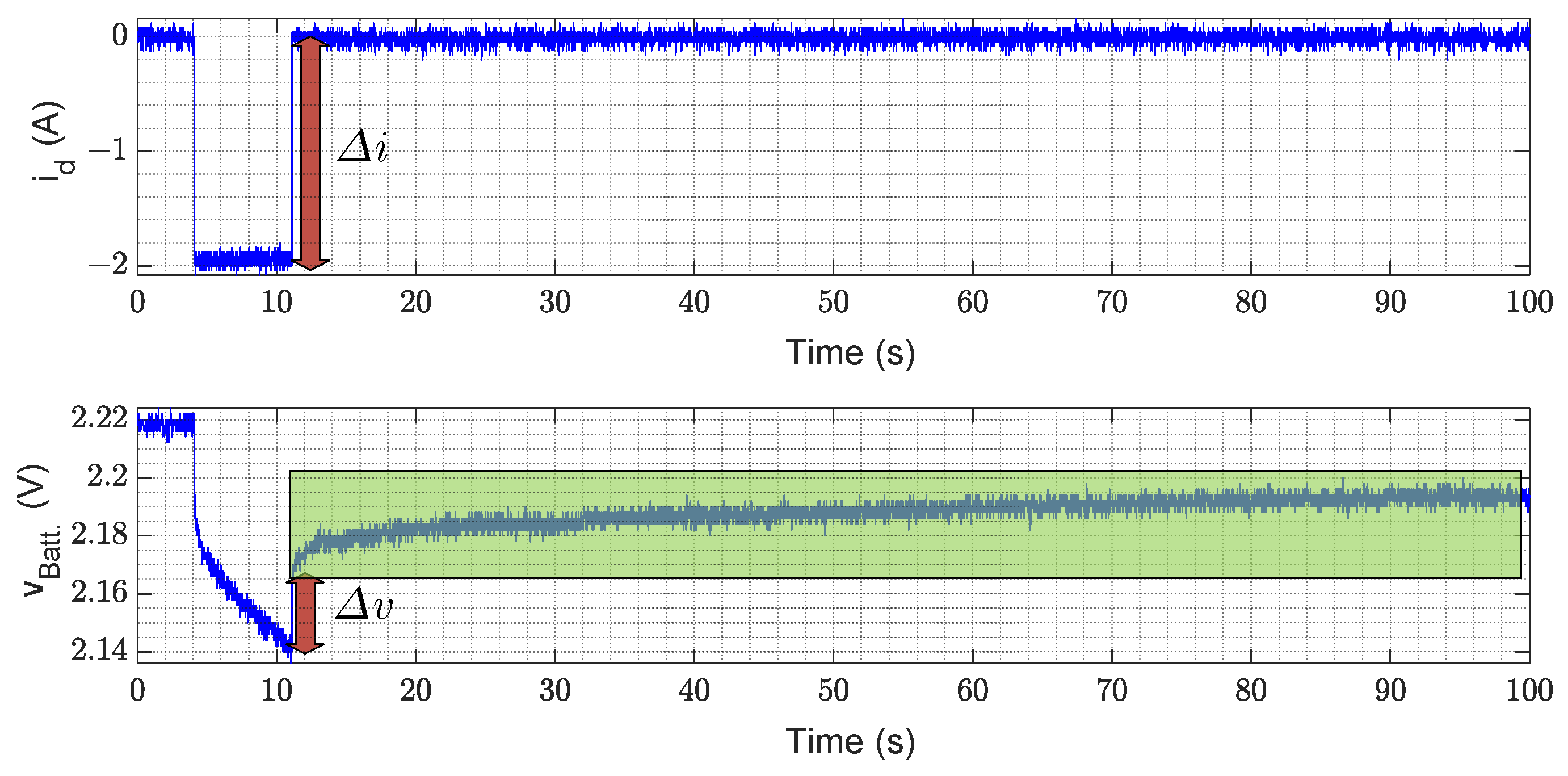
  • Dynamic response parameters: R 0 represents the instantaneous voltage/current change and the other elements splits the transient response into the time constants [30].
  • Battery states: These represent the energy storage and the modification of the battery response [31].
To estimate v O C , the SOC should be calculated first using an auxiliary variable v S O C [ 0 , 1 ] . A simple method used is Coulomb Counting (CC), as described by (1).
v S O C ( t ) = v S O C ( 0 ) 0 t η · i · d t C a v a i l a b l e
where v S O C ( t ) is the SOC voltage at the time t, v S O C ( 0 ) is the SOC voltage at t = 0 s, η is a correction factor where η = 1 since their values are close to this number, and C a v a i l a b l e is the remaining capacity in Ah.
One of the ways to approximate this correlation is through a discharge by controlled pulses until complete battery discharge [15,32]. Figure 2 shows the pulse discharge suggested. As the discharge pulses are carried out at 0.2 C and the time that each pulse lasts is known, the percentage of charge remaining after each pulse can be estimated. The points marked with a star indicate the v b a t t value, which better approximates the corresponding v O C located in the voltage stabilization point [33]. The data obtained allow the approximation of the relationship between the v S O C and the v O C , as shown in Table 2 and displayed in Figure 3 in triangles. To proceed with the next stages of the paper, it is necessary to have continuous SOC behavior. To achieve this, a fifth-order function can be used to fit the estimated v S O C using MATLAB 2018b. The result is displayed in Figure 3 as a continuous line.
The obtained fifth-order polynomial is:
v O C = 2.357 · ( v S O C ) 5 5.963 · ( v S O C ) 4 + 5.624 · ( v S O C ) 3 2.442 · ( v S O C ) 2 + 0.6952 · ( v S O C ) + 1.912
Under what was described above, the v O C value is considered to be known in advance; the parameterization process used for the EEC is described below.

2.1. Model Parameter Identification

For the EEC model, it is necessary to parameterize R 0 , R 1 , R 2 , R 3 , C 1 , C 2 , and C 3 . The method proposed by Plett [7] is based on the response to a discharge pulse. This test is illustrated in Figure 4, where the values of Δ i and Δ v correspond to the instantaneous changes, obtaining the value of R 0 using Ohm’s law from these.
From the information in the green box, a function of the form (3) is obtained through exponential regression in MATLAB 2018b.
f ( x ) = a e b t + c e d t + f e g t
Considering v b a t t , i, R 0 , and v O C as known, leaving only the elements on the right-hand side of Equation (4), we relate the terms on the right side of Equations (3) and (4)
v b a t t v O C i R 0 = R 1 i e t / ( R 1 C 1 ) R 2 i e t / ( R 2 C 2 ) R 3 i e t / ( R 3 C 3 )
For a Power Sonic PS260 VRLA battery from 2 V to 6 Ah, the parameters obtained are shown in Table 3.

2.2. Equivalent Electric Circuit Model

Using the obtained parametrization data and incorporating the estimate of v S O C given in (1), the state-space model (5) is constructed; for this, Kirchhoff’s laws are applied to the EEC model in Figure 1 [7].
x ˙ = A x + B i v b a t t = h ( x ) + D i
Defining the vector x and matrices A , B , and D as (6) [7].
x = v 1 v 2 v 3 v S O C ; A = 1 τ 1 0 0 0 0 1 τ 2 0 0 0 0 1 τ 3 0 0 0 0 0 ; B = 1 C 1 1 C 2 1 C 3 1 C a v a i l a b l e ; D = R 0 ;
Likewise, h ( x ) is Function (7) and τ 1 = R 1 · C 1 , τ 2 = R 2 · C 2 , and τ 3 = R 3 · C 3 .
h ( x ) = v 1 v 2 v 3 + v O C
h ( x ) is a nonlinear function because it contains the v O C polynomial Equation (2).
Equation (8) was used to estimate the value of C a v a i l a b l e , which is obtained from CC [7].
C a v a i l a b l e = 1 Δ v S O C t 0 t 1 i ( t ) d t
where t 0 is the initial time for evaluation, t 1 is the final time, and Δ v S O C is the change in the v S O C between t 0 and t 1 . It is important to establish that Δ v S O C 0 .
The model response shown in Figure 5 is obtained from the nonlinear model. For this purpose, a charge and discharge cycle at 0.2 C was used in a battery without wear. Figure 5a shows the measured voltage in a cycle, represented by the blue line, and the estimated voltage with the proposed model, represented by the red line, and Figure 5b shows the v S O C calculated by CC.
The results show similar trends between the measured and simulated results. However, the values of the resistors and capacitors change with respect to the SOC and SOH variations, which will increase the deviation between the model and actual measurements. To deal with that situation, another approach is formulated in Equation (9) where a model including all the parametric variations along the SOH is established to propose a nonlinear observer whose purpose is to guarantee the process of detecting typical and atypical parametric variations
x ˙ = A s b x + B s b u x ˙ = A s e x + B s e u y = h ( x ) + D s b u y = h ( x ) + D s e u x ˙ = A f b x + B f b u x ˙ = A f e x + B f e u y = h ( x ) + D f b u y = h ( x ) + D f e u
where the subscript s corresponds to the beginning of the SOH, f corresponds to the end of the SOH, b represents 100% of the SOC, and e represents 0% of the SOC.
The SOH is estimated by using the battery capacity in ampere-hours according to Equation (10):
S O H ( % ) = C a v a i l a b l e C n o m × 100 %
where C n o m is the nominal capacity given on the datasheet, and C a v a i l a b l e is the available capacity estimated by Formula (8).
SOH is a fundamental parameter for detecting battery degradation. The mechanisms that create that degradation are divided into corrosion, hard sulfation, and active material loss. As it was established, CC is a typical method for estimating SOH and SOC; however, that technique has some practical limitations such as:
(a)
It is dependent on the current sensor precision.
(b)
It is susceptible to deviations created by different initial conditions.
(c)
The integral action is prone to bias depending on cumulative errors developed for offsets, which forces the use of anti-windup techniques.
All the previous drawbacks can put the integrity of the battery at risk.
To avoid the aforementioned and take care of the batteries, it is proposed to use an observer by using (9). The observer selected has a non-linear output map according to the state space (5). This observer is explained in [34], and has already been tested in lithium-ion batteries [35].
The selected observer is also robust against parameter variations since the correction vector will adjust the model to follow the measures. In this way, the observer’s dynamics will compensate for the effect of the parametric changes within the observed states. This observer will not only lead to correct monitoring of the system but also allows for knowing the evolution of the dynamic response throughout its useful life.

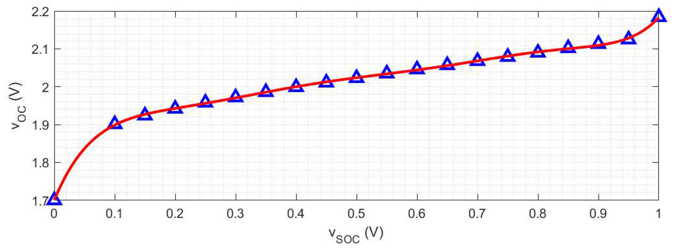
2.3. Nonlinear State-of-Charge Observer

Equation (11) shows the observer structure used. Note that the structure of the selected observer is linear for matrices A and B.
x ^ ˙ = A · x ^ + B · u + H · h T ( x ^ ) ( y y ^ ) y ^ = h ( x ^ ) + D · u
where h ( x ) is the partial derivative from h ( x ) with respect to the vector of states, and H is the correction vector. The error dynamics between the system and the observer are defined as (12).
e ˙ x = x ˙ x ^ ˙ = ( A H h T h ) e x
This observer needs to fulfill some conditions according to [34]:
Corollary 1 
(Zero eigenvalues). A is allowed to have one eigenvalue with R e { λ j ( A ) } = 0 and all other eigenvalues R e { λ i ( A ) } < 0 , with the observer structure (11) where the matrix H is a symmetric and positively defined solution for the Lyapunov Equation (13).
A T H 1 + H 1 A = Q
where the design matrix Q is symmetric and positive semidefinite, and r a n k ( A ) r a n k ( Q ) .
Proof. 
Supose that the matrix Q as (14):
Q = 2 / k 1 0 0 0 0 2 / k 2 0 0 0 0 2 / k 3 0 0 0 0 0
It is substituted into Equation (13) like the matrix A shown in (6), obtaining expression (15).
2 H 1 / τ 1 0 0 0 0 2 H 2 / τ 2 0 0 0 0 2 H 3 / τ 3 0 0 0 0 0 = 2 / k 1 0 0 0 0 2 / k 2 0 0 0 0 2 / k 3 0 0 0 0 0
where H 1 , H 2 , H 3 , and H 4 are the elements of the correction vector H . Finding the values of the vector H , as indicated in (16), element H 4 is a free element, where all are positive constants.
H 1 = τ 1 k 1 H 2 = τ 1 k 2 H 3 = τ 1 k 3 H 4 = k 4
The selected Lyapunov function is (17):
V ( e x ) = e x T H 1 e x
Therefore, the derivative of the function is described as (18):
V ˙ ( e x ) = e ˙ x T H 1 e x + e x T H 1 e ˙ x
Substituting Equation (12) in (18) is expressed as (19):
V ˙ ( e x ) = e x T A T H 1 e x + e x T H 1 A e x e x T h T h H T H 1 e x e x T h T h H H 1 e x
Using Equation (13) and considering that matrix H is symmetric and positively defined, we can ensure that H = H T and simplify Equation (19) in (20).
V ˙ ( e x ) = e x T ( Q ) e x e x T ( 2 h T h ) e x = e x T ( Q + h T h ) e x
where the matrix Q + h T h is defined as (21).
Q + h T h = 2 1 + H 1 1 1 v O C v S O C 1 1 + H 2 1 v O C v S O C 1 1 1 + H 3 v O C v S O C v O C v S O C v O C v S O C v O C v S O C ( v O C v S O C ) 2
Given matrix (21), it is necessary to guarantee that it is positive definite, so the Sylvester criterion is used [36], taking all the superior principal submatrices and calculating their determinants ( Δ 1 , Δ 2 , Δ 3 , and Δ 4 ) (22).
Δ 1 = 2 ( 1 + H 1 ) Δ 2 = 4 ( H 1 + H 2 + H 1 H 2 ) Δ 3 = 8 ( H 1 H 2 + H 1 H 3 + H 2 H 3 + H 1 H 2 H 3 ) Δ 4 = 16 ( H 1 H 2 H 3 v ˙ O C )
Considering that H 1 , H 2 , H 3 , and H 4 are positive and that the derivative of v O C is positive on the interval ( [ 0 , 1 ] ), it is known that the determinants of the principal submatrices are positive. Therefore, (21) is negative definite, concluding in this way that the derivative of the proposed Lyapunov function is positive, so the error is asymptotically stable. □
Corollary 2 
(Nonlinear condition). The nonlinear function h ( x ) and its derivative h ( x ) are Lipschitz.
Proof. 
Consider that h ( x ) and h ( x ) are polynomial functions; hence, it is of interest to demonstrate that they are locally Lipschitz using the inequality (23) [37].
h ( x ) x L x R
This indicates that the Lipschitz constant should be higher than any of the Jacobian supremes in the closed interval where the SOC has a physical meaning ( [ 0 , 1 ] ).
For this case, the partial derivative of the function h ( x ) is nonlinear only in its partial derivative to v S O C , resulting in the polynomial Equation (24).
v O C v S O C = 11.785 · ( v S O C ) 4 23.852 · ( v S O C ) 3 + 16.872 · ( v S O C ) 2 4.884 · ( v S O C ) + 0.6952
Since the resulting function is polynomial and is bounded to a closed interval, all of its contra-domains are finite by definition, allowing us to conclude that there exists a value greater than any element belonging to the contra-domain of the bounded function. L : h ( x ) x L x R . □
For this case, the values of H 1 = 0.6 , H 2 = 0.6 , H 3 = 0.6 , and H 4 = 0.2 were selected, respecting the above corollaries.

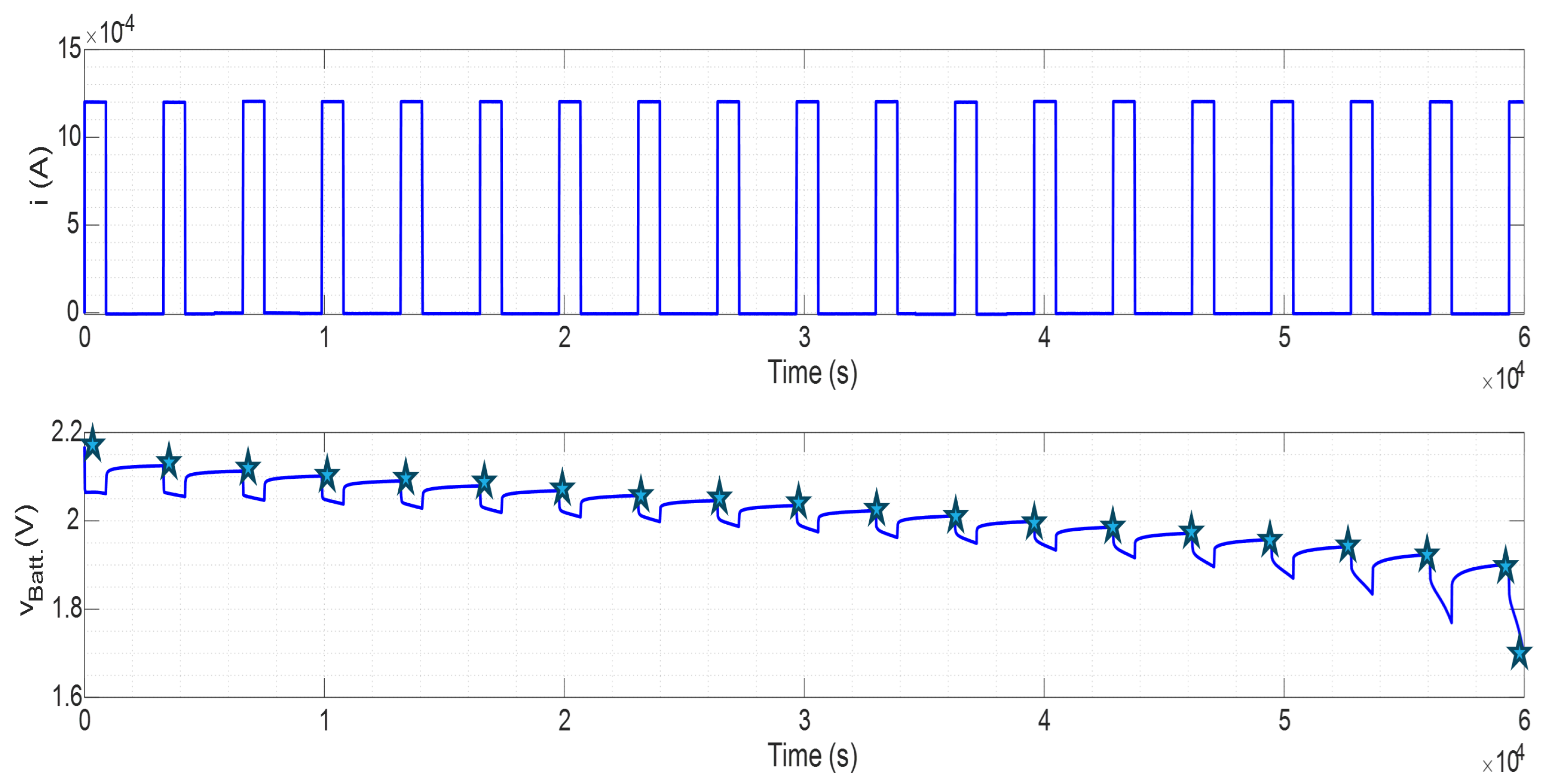
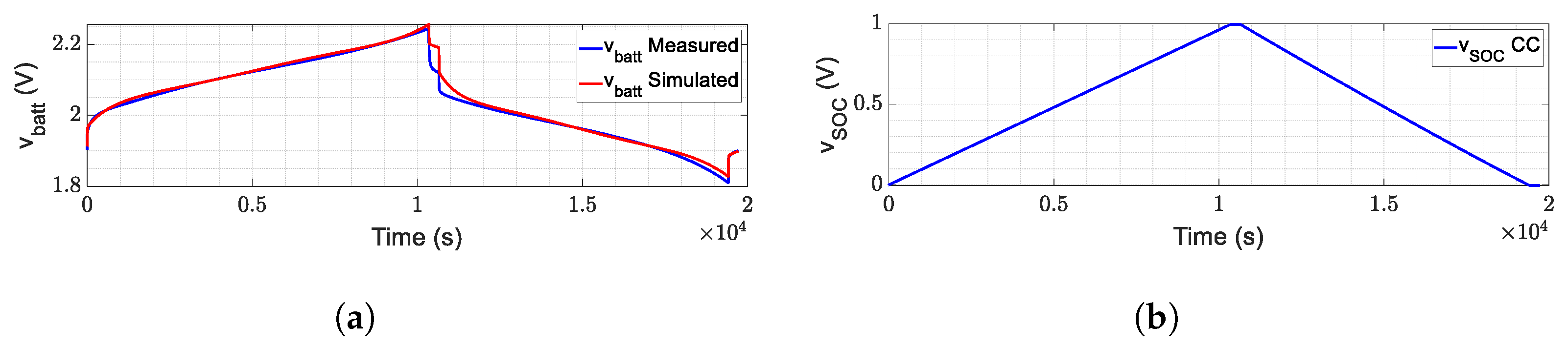
3. Experimental Validation

Once the observer demonstrations have been completed, an experimental evaluation of its feasibility and advantages compared to the CC technique shall be presented.
Batteries were tested with 0, 25, 50, 100, 150 and 200 aging cycles. For this, the batteries were subjected to a charge and discharge profile that responds to the IEC 60095-1 standard [38], as shown in Figure 6. The voltage limits are established according to the discharge characteristics given by the manufacturer, with the maximum operating voltage being 2.24 V and the minimum voltage being 1.8 V [39].
The first thing to validate is the observer behavior in deteriorating conditions and compare it with the model using only Coulomb Counting. For this, Figure 7a shows the battery voltages obtained, and it can be seen that the observer voltage accurately tracks the measured voltage programmed in MATLAB. Figure 7b shows the SOC with both methods. Additionally, Table 4 shows a quantitative comparison of the moments marked as of interest.
According to the results depicted in Figure 7, the following statements are formulated:
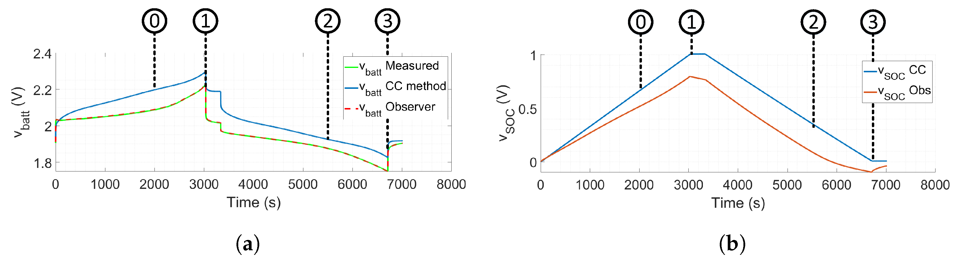
  • Marker 0 shows that the observer has a better performance when tracking the voltage measurement.
  • Marker 1 shows how the CC estimates more SOC than the observer.
  • Marker 2 shows how the CC estimates 32% of the SOC when the observer estimates 0%.
  • Marker 3 shows how the CC estimates the end of SOC when the battery has been over-discharged since Marker 2.
Due to these conditions, it is concluded that CC delivers results close to what was expected. However, it exposes the battery to possible under-charge or over-discharge conditions by increasing its aging—a detail that the observer corrects.
Another point to evaluate is the inclusion of the variations in the dynamics due to parametric changes, which are added to the different states of the model. The states correspond to the voltage in the R C arrangements, plotting the battery without aging and the battery with 200 aging cycles, and the results are shown in Figure 8. These results come from the charge/discharge test previously described, where the blue lines correspond to the model using CC and the red lines correspond to the observer.
Note that the model response with CC presents little changes even when evaluating batteries with different aging states. The observer in Figure 8a–c shows minor variations throughout the charge and discharge; the differences between the model with CC and the observer correspond to the variation in the parameters due to the previously discussed changes in the SOC.
In the same way, Figure 8d–f show how the observer variations are more pronounced than the previous ones due to parametric changes due to aging. The results shown by the observer are consistent with what is described in the literature and prove that the observer includes the parametric variations in a single model. In this case, the differences between the model and the observer increase since the greater the parametric changes are, the greater the aging.
According to the previous results, tests were carried out on different batteries with different aging points measured in discharge cycles, extracting from the model the behavior of the voltage in the different states, producing the results shown in Figure 9. In this way, the evolution of the system’s dynamic response can be observed, approximating the ideal aging trend observable as:
  • The time it takes to complete the charge is increasingly shorter due to capacity lost.
  • v 3 has more obvious differences because it represents the most significant time constant.
  • The transient movements are abrupt as the battery ages due to parametric variation.
  • The most relevant changes occurred at the beginning and end of SOC due to the non-linear response.
  • Initial overshoot appears in the v 2 and v 3 graphs.
Figure 9a–c correspond to the state response during the charging process following the previously mentioned tendencies. On the other hand, Figure 9d–f correspond to the voltages of the state variables in the discharge process; in addition to following the trends described above, it is highlighted that the transient has more noticeable changes due to the natural electrochemical reaction tendency, and as the battery ages, the voltage amplitude is lower at the end of the SOC—notable in v 1 .
It is important to note in Figure 9 that all the graphs have a consistent behavior; it is evident that the parametric changes deform the response, but the trend remains monotonous throughout the useful life. It also becomes clear that as age increases, resistance values increase, observable in the plotted overshoots, and the time constants decrease, visible in the abrupt transients, validating that the use of the observer shows the changes produced by the SOH and the parametric variation.
With the evidence previously presented, the modeling of the battery is postulated according to Equation (25), where aging is treated as a multiplicative fault, modifying the parameters of the model, where said multiplicative faults depend on aging.
x ˙ = ( A + Δ A F ) · x + ( B + Δ B F ) · u y = h ( x ) + ( D + Δ D F ) · u
where the matrices Δ A F , Δ B F , Δ D F represent the changes in the system parameters due to the advance in the SOH, described in the form (26).
( A + Δ A F ) = 1 τ 1 + Δ τ 1 0 0 0 0 1 τ 2 + Δ τ 2 0 0 0 0 1 τ 3 + Δ τ 3 0 0 0 0 0 ; ( B + Δ B F ) = 1 C 1 + Δ C 1 1 C 2 + Δ C 2 1 C 3 + Δ C 3 1 C u s a b l e ; ( D + Δ D F ) = R 0 + Δ R 0 ;
where R 0 , C 1 , C 2 , C 3 , τ 1 , τ 2 , and τ 3 are the time-invariant parts of the model and only depend on the SOC, while Δ R 0 , Δ C 1 , Δ C 2 , Δ C 3 , Δ τ 1 , Δ τ 2 , and Δ τ 3 depend on the aging, thus defining the effect of aging as a multiplicative element of parametric modification.
To obtain the additive terms of matrix Δ A F and Δ B F , it was considered that the changes would modify the term found in the denominator, and it is sought to separate said term into the sum of two fractions where one of them is the original term of matrix A , as shown in Equation (27), where the term a 11 of matrix Δ A F will be exemplified; however, the procedure is the same for all terms.
1 τ A + Δ τ A = 1 τ A + a 11
To obtain the searched value, term a 11 is cleared, as shown in Equation (28), this same procedure is repeated for the rest of the aforementioned terms.
a 11 = 1 τ A + Δ τ A + 1 τ A = Δ τ A τ A ( τ A + Δ τ A )

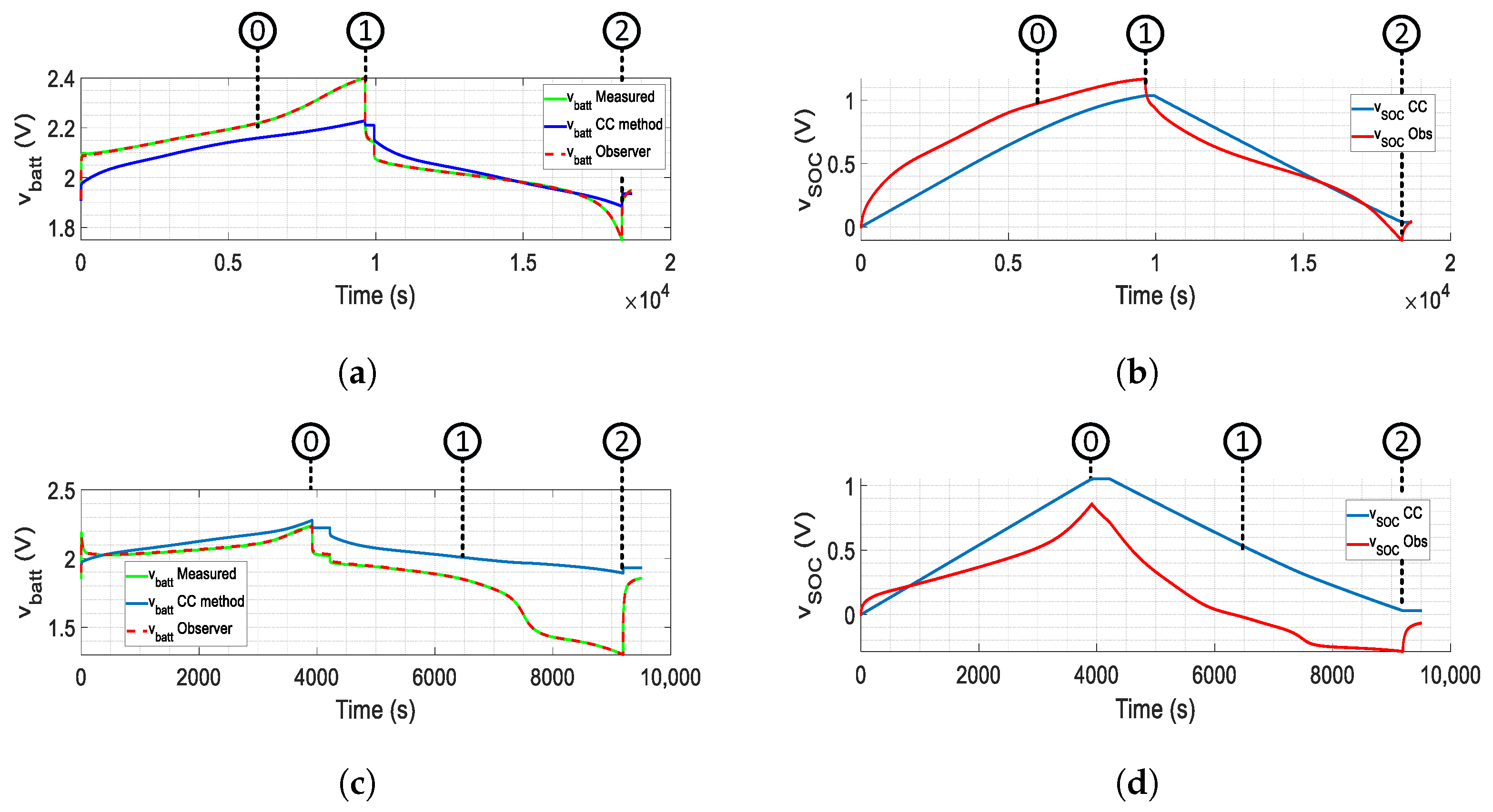
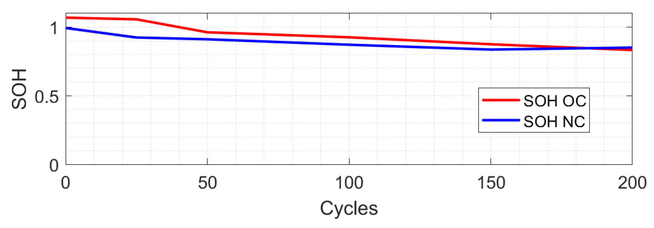
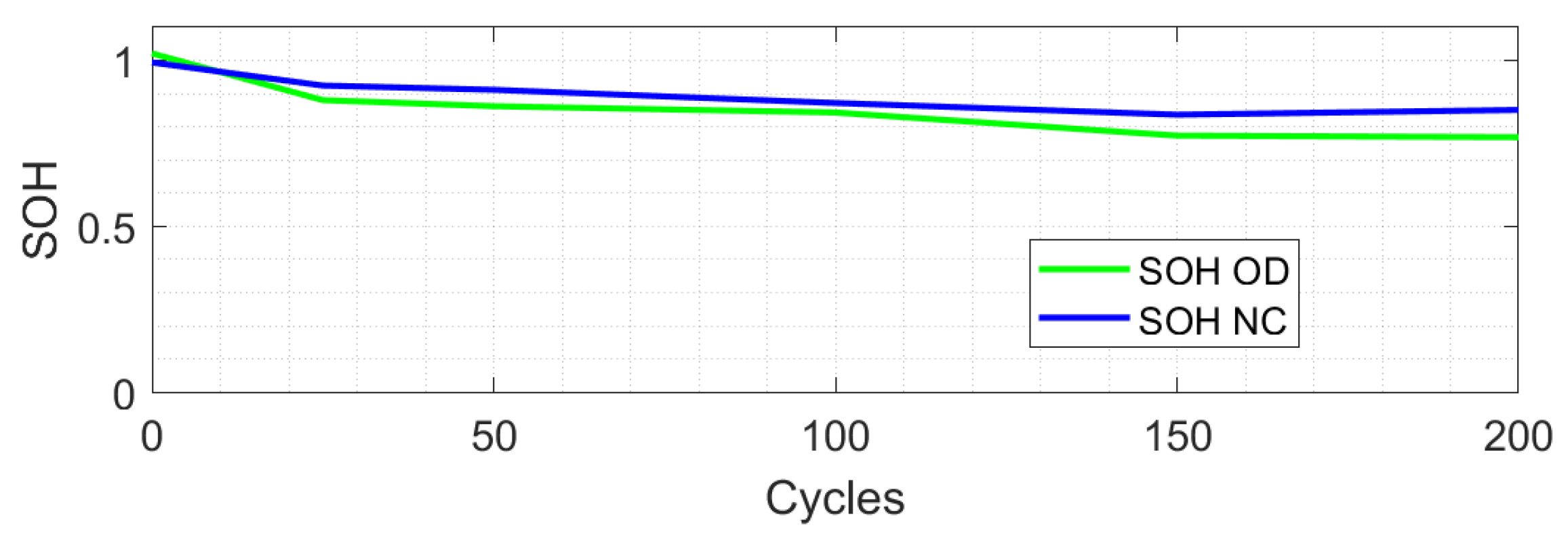
4. Over-Charge and Over-Discharge Test

For the sake of proving the suitability of model (26) in extreme conditions of misuse of the batteries, controlled tests of overcharging and over-discharging a set of batteries were performed accordingly with the Figure 6 profile during complete battery life.
For this test, it is observed that the observer tracking is better than the CC model, where Figure 10a,b show the voltages and SOC levels obtained in over-charge, and Figure 10a,b show the voltages and SOC levels obtained in over-discharge. In the same way, Table 5 gives a numerical comparison of the responses. According to the evaluation of the results, the following conclusions are made:
  • The over-charge case in marker 0 shows how the observer identifies that the battery is over 100% of the SOC.
  • The over-charge case marker 1 shows a significant difference from the CC model.
  • The over-discharge case in marker 1 shows how the observer identifies that the battery falls to 0% of SOC.
  • The over-discharge case Marker 2 shows a significant difference from the CC model.
  • Over-charge marker 2 and over-discharge marker 0 show that the CC model has a close approach.
Subsequently, the batteries subjected to aging with over-charge levels were analyzed. It was found that the evolution of SOH under over-charge (SOH OC) tends to grow above 100%, as shown in Figure 11 with a red line, and compared to the evolution of SOH under normal conditions (SOH NC) by the manufacturer in the blue line, it does not show superior aging.
These results make it possible to infer a difference when comparing the SOH. However, these are subtle and could pass as a battery subjected to normal discharge. That is why the states of the proposed observer are analyzed, producing the results of Figure 12, which shows the response to the charge and discharge of the battery with 200 cycles of aging under over-charge conditions (red line), the reaction of a battery with 200 cycles of aging under normal conditions (blue dashed line), and the reaction of a battery without aging conditions (blue line).
Figure 12a–c show the response of the state variables to the load, where essential differences can be observed; first, there is an overshoot greater than the expected behavior in the three graphs, becoming evident in v 3 . In the same way, the amplitude of the graphs before finishing the load decreases significantly, which is evident in v 1 . On the other hand, Figure 12d–f show the response in the discharge; it is possible to find a behavior outside of what was expected. In this case, contrary to the load graphs, it is not shown on impulse. On the contrary, the charts show a smooth behavior, which indicates that the variations in the time constants have been smaller than those obtained with normal aging, which becomes relevant in the first moments after the change in current. This allows us to conclude that changes in the smallest time constant and the elements of the instantaneous response will demonstrate actual aging due to over-charge.
In addition, the same analysis was carried out on aged over-discharge batteries. Figure 13 shows with a blue line the evolution of the SOH of the batteries aged under normal conditions (SOH CN), while the green line shows the behavior of the SOH of the aged batteries under over-discharge conditions (SOH OD).
In this case, the SOH advances faster when the battery is subjected to over-discharge conditions, decaying 10% more than the normally aged battery, demonstrating that the SOH can detect this misuse.
Complementary to the SOH, the responses of the observer’s state variables were analyzed, obtaining Figure 14. The reaction of a battery without aging is shown with a blue line. The response of a battery with 200 aging cycles in conditions recommended by the manufacturer is shown with a blue dashed line, and the reaction of a battery with 200 aging cycles in over-discharge conditions is shown with a green line.
Figure 14a–c show the results of this test during charging, where it can be noted that the battery response has a behavior similar to the proposed limits, differentiated by an initial overshoot with a very short duration. On the other hand, Figure 14d–f show the response to the discharge; in this case, the response is similar to the proposed limits both in the instantaneous response and in the transient of the first moments. However, after the first moments, the behavior of the transient is more abrupt than that of the proposed limits. In this way, it is possible to conclude that over-discharge is associated with the largest instantaneous changes and time constants.
It is possible to conclude that the extraction of additional information can detect aging due to misuse in greater detail than the SOH, where in cases of aging due to over-charge, it does not detect the correct level of aging. At the same time, the observed states show signs of aging. Likewise, it is possible to associate the responses of the conditions of misuse with time variables.
  • Both the effects of over-charge and over-discharge modify the instantaneous response, which is directly related to the loss of active material. By rapidly wearing out the battery, the material is forced to lose effectiveness before the expected time.
  • The over-charge conditions are strongly reflected in the reactions with a lower time constant, being associated with the effects of the electrical double layer and corrosion.
  • Over-discharge conditions have a longer response time, making it possible to associate them with diffusion effects and hard sulfation.
With these new conclusions, it is possible to give meaning to the multiplicative faults of the proposed model (25), which do not provide information on the detection of aging; this does not eliminate or invalidate the detection of SOH; on the contrary, it provides additional information to improve the detection.
  • Δ R 0 
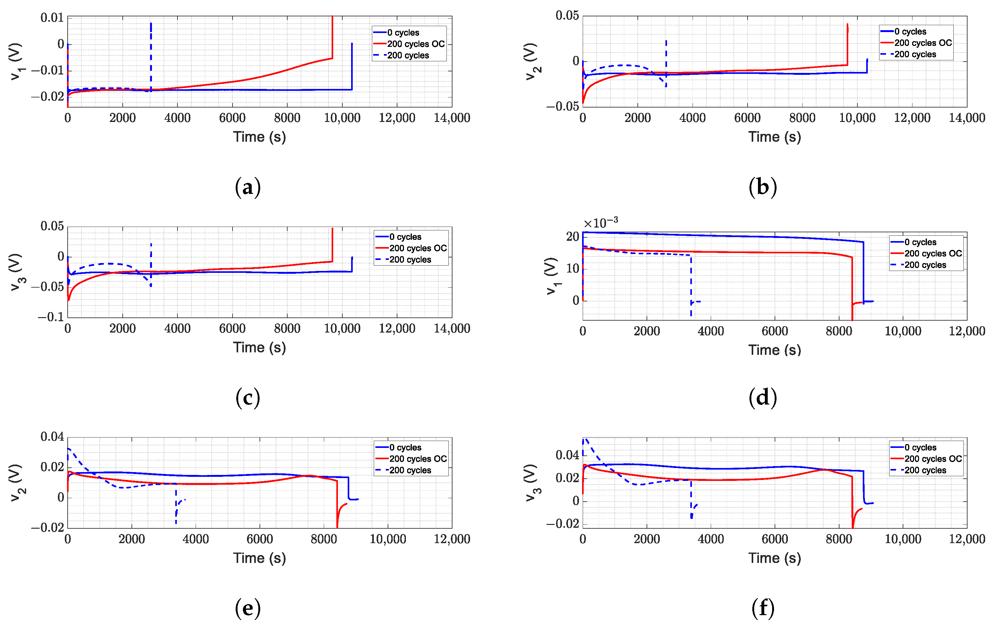
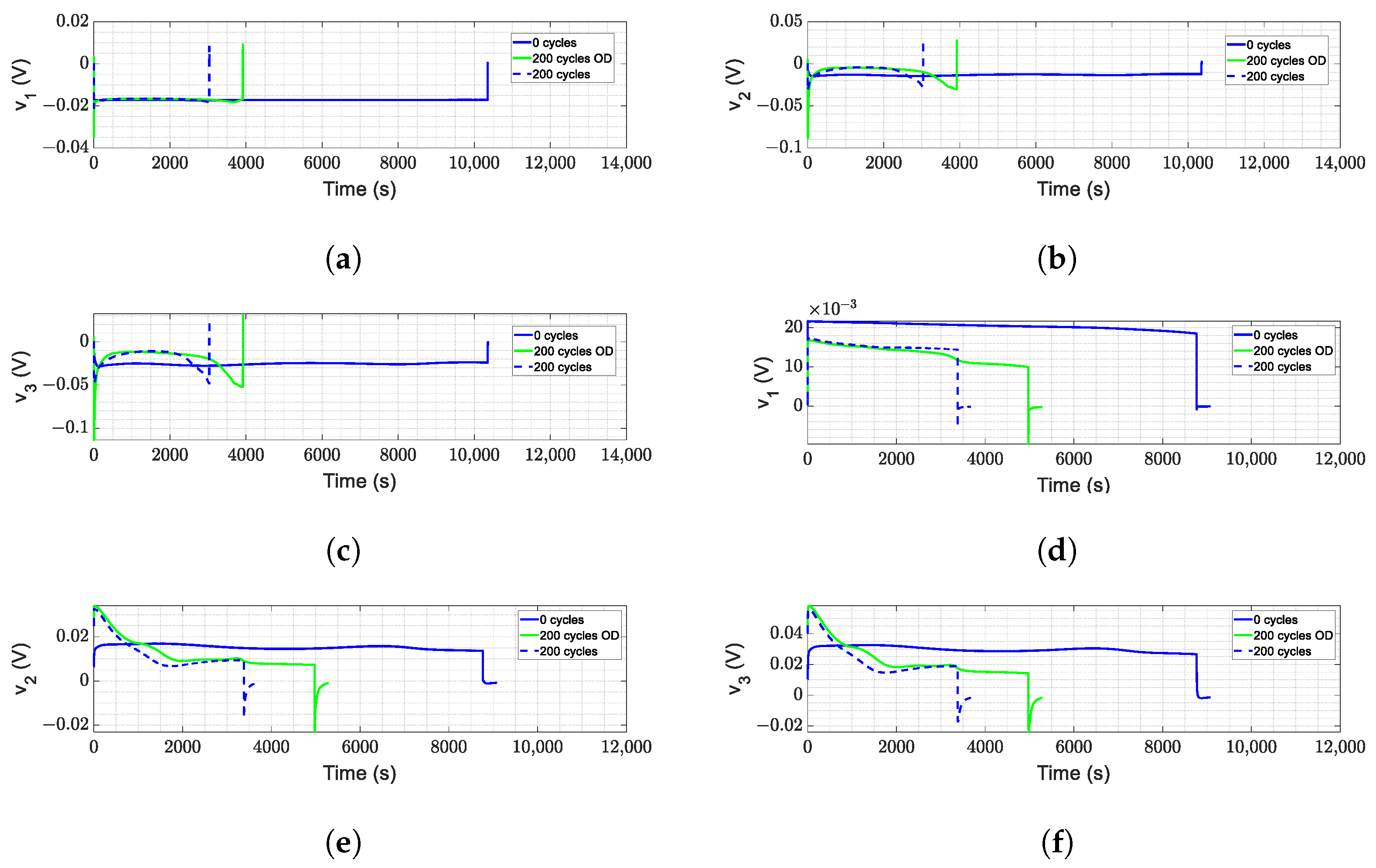
corresponds to instantaneous changes graphically; this is reflected in the overshoots in Figure 9, both in charging and discharging, increasing progressively with aging; in the same way, it appears more aggressively with over-charge and over-discharge, particularly when charging the battery.
  • Δ τ 1 and Δ C 1 correspond to the changes present in the smallest time constants. The values are modified in all cases; however, it has a relevant change in the over-charge in Figure 12 since, during the charge, it is in these elements where the drop in the amplitude has a noticeable change in proportion to its expected nominal values. Likewise, during discharge, this time constant dampens the first moments in conjunction with the absence of the expected overshoot.
  • Δ τ 2 and Δ C 2 correspond to the reactions with the middle time constant; in this case, the variations in these elements are progressive with respect to aging, and although it showed changes between normal aging and aging due to misuse, it does not reveal such compelling information. However, together with the rest of the variations, it allows us to validate that they are changes due to misuse or errors in the estimation.
  • Δ τ 3 and Δ C 3 correspond to variations in the slower time constants, and it is these changes that mainly contribute to the voltage oscillations during charging and discharging. These effects are present during aging under normal conditions and are accentuated during aging due to over-discharge and, on the contrary, are attenuated during aging due to over-charge.

5. Conclusions

Traditionally, battery life is determined by the State of Health (SOH). Still, this article shows that it is possible to have more information that allows us to distinguish between normal aging and misuse conditions. To this end, this article presents the development of a mathematical model in the state space of a three-tank equivalent circuit capable of representing these two conditions, normal and misused, and providing more information than just the SOH through multiplicative terms on the state and the input. The importance of this model can be observed by analyzing the experimental results, showing how the performance of state variables reflects that the batteries are subjected to unusual stress. This implies that the integrity of the battery is at risk.
It can be observed that the use of the SOH provides aging information; however, in the presence of misuse conditions, it is not able to make a detailed diagnosis and may not even notice such conditions. Therefore, the methodology proposed in this work seeks to provide additional information so that, in conjunction with the SOH, it is possible to distinguish conditions of misuse, preventing a failure in advance.
The proposed methodology shows how the behavior of a battery subjected to overcharge and over-discharge maintains a similar operation to normal conditions. However, the states of the proposed model and observer show how their performance reveals the irregularity of the charging and discharging process.
With aging treated as a multiplicative fault, the mathematical space-state model allows us to approach aging as a parametric change, marking a step in detecting aging from a different standpoint.

Author Contributions

H.V.-A.: conceptualization, data curation, formal analysis, methodology, validation, investigation, visualization, software, writing—original draft. N.V.-C.: conceptualization, formal analysis, supervision, funding acquisition, writing—review and editing, project administration. C.A.N.-G.: conceptualization, funding acquisition, validation, writing—review and editing, resources, supervision, methodology. J.S.-R.: funding acquisition, validation, resources, supervision. All authors have read and agreed to the published version of the manuscript.

Funding

CONAHCYT funded this contribution through project CF 2019/1311344, project A1-S-29705, and scholarship 1010810.

Data Availability Statement

The raw data supporting the conclusions of this article will be made available by the authors upon request.

Acknowledgments

The authors would like to thank Schweitzer Engineering Laboratories for providing the digital infrastructure. In the same way, we thank the UASLP electric vehicle laboratories for the facilities provided for this research.

Conflicts of Interest

The authors declare no conflicts of interest.

Abbreviations

The following abbreviations are used in this manuscript:
EECEquivalent electric circuit
CCCoulomb Counting
SOCState of charge
SOHState of health
VRLAValve regulated lead-acid
Nomenclature
Δ i Instantaneous change in current [A]
Δ v Instantaneous change in voltage [V]
η Correction factor
C 1 Capacitance of the first R C arrangement [F]
C 2 Capacitance of the second R C arrangement [F]
C 3 Capacitance of the third R C arrangement [F]
C a v a i l a b l e Remaining capacity [Ah]
C n o m Battery nominal capacity [Ah]
iDemanded current [A]
R 0 Serial resistance [ Ω ]
R 1 Resistance of the first R C arrangement [ Ω ]
R 2 Resistance of the second R C arrangement [ Ω ]
R 3 Resistance of the third R C arrangement [ Ω ]
tDesired time [s]
t 0 Initial time of evaluation [s]
t 1 Final time of evaluation [s]
v 1 Voltage in parallel arrangement R 1 C 1 [V]
v 2 Voltage in parallel arrangement R 2 C 2 [V]
v 3 Voltage in parallel arrangement R 3 C 3 [V]
v b a t t Terminal voltage [V]
v O C Open Circuit Voltage [V]
v S O C State of Charge Voltage [V]

References

  1. Sharma, S.; Panwar, A.K.; Tripathi, M. Storage technologies for electric vehicles. J. Traffic Transp. Eng. 2020, 7, 340–361. [Google Scholar] [CrossRef]
  2. Sanguesa, J.A.; Torres-Sanz, V.; Garrido, P.; Martinez, F.J.; Marquez-Barja, J.M. A review on electric vehicles: Technologies and challenges. Smart Cities 2021, 4, 372–404. [Google Scholar] [CrossRef]
  3. Pan, Z.; Quynh, N.V.; Ali, Z.M.; Dadfar, S.; Kashiwagi, T. Enhancement of maximum power point tracking technique based on PV-Battery system using hybrid BAT algorithm and fuzzy controller. J. Clean. Prod. 2020, 274, 123719. [Google Scholar] [CrossRef]
  4. Maddukuri, S.; Malka, D.; Chae, M.S.; Elias, Y.; Luski, S.; Aurbach, D. On the challenge of large energy storage by electrochemical devices. Electrochim. Acta 2020, 354, 136771. [Google Scholar] [CrossRef]
  5. Haider, S.N.; Zhao, Q.; Li, X. Data driven battery anomaly detection based on shape based clustering for the data centers class. J. Energy Storage 2020, 29, 101479. [Google Scholar] [CrossRef]
  6. IEEE-650-5318; IEEE Standard for Qualification of Class 1E Static Battery Chargers, Inverters, and Uninterruptible Power Supply Systems for Nuclear Power Generating Stations. IEEE: Piscataway, NJ, USA, 2018. Available online: https://standards.ieee.org/ieee/650/5318/ (accessed on 1 July 2021).
  7. Plett, G.L. Battery Management Systems, Volume I: Battery Modeling; Artech House: New York, NY, USA, 2015; Volume 1. [Google Scholar]
  8. Lai, C.S.; Locatelli, G.; Pimm, A.; Wu, X.; Lai, L.L. A review on long-term electrical power system modeling with energy storage. J. Clean. Prod. 2021, 280, 124298. [Google Scholar] [CrossRef]
  9. May, G.J.; Davidson, A.; Monahov, B. Lead batteries for utility energy storage: A review. J. Energy Storage 2018, 15, 145–157. [Google Scholar] [CrossRef]
  10. Yu, Y.; Mao, J.; Chen, X. Comparative analysis of internal and external characteristics of lead-acid battery and lithium-ion battery systems based on composite flow analysis. Sci. Total. Environ. 2020, 746, 140763. [Google Scholar] [CrossRef]
  11. Ahuja, R.; Blomqvist, A.; Larsson, P.; Pyykkö, P.; Zaleski-Ejgierd, P. Relativity and the lead-acid battery. Phys. Rev. Lett. 2011, 106, 018301. [Google Scholar] [CrossRef]
  12. Levy, S.C.; Bro, P. Battery Hazards and Accident Prevention; Springer Science & Business Media: Berlin/Heidelberg, Germany, 1994. [Google Scholar]
  13. Rand, D.A.J.; Holden, L.; May, G.; Newnham, R.; Peters, K. Valve-regulated lead/acid batteries. J. Power Sources 1996, 59, 191–197. [Google Scholar] [CrossRef]
  14. Huang, S.C.; Tseng, K.H.; Liang, J.W.; Chang, C.L.; Pecht, M.G. An online SOC and SOH estimation model for lithium-ion batteries. Energies 2017, 10, 512. [Google Scholar] [CrossRef]
  15. Plett, G.L. Battery Management Systems, Volume II: Equivalent-Circuit Methods; Artech House: New York, NY, USA, 2015; Volume 2. [Google Scholar]
  16. Sun, S.; Sun, J.; Wang, Z.; Zhou, Z.; Cai, W. Prediction of battery soh by cnn-bilstm network fused with attention mechanism. Energies 2022, 15, 4428. [Google Scholar] [CrossRef]
  17. Liu, W.; Xu, Y.; Feng, X.; Wang, Y. Optimal fuzzy logic control of energy storage systems for V/f support in distribution networks considering battery degradation. Int. J. Electr. Power Energy Syst. 2022, 139, 107867. [Google Scholar] [CrossRef]
  18. Hughes, M.; Barton, R.; Karunathilaka, S.; Hampson, N. The estimation of the residual capacity of sealed lead-acid cells using the impedance technique. J. Appl. Electrochem. 1986, 16, 555–564. [Google Scholar] [CrossRef]
  19. Yu, R.; Liu, G.; Xu, L.; Ma, Y.; Wang, H.; Hu, C. Review of Degradation Mechanism and Health Estimation Method of VRLA Battery Used for Standby Power Supply in Power System. Coatings 2023, 13, 485. [Google Scholar] [CrossRef]
  20. Badeda, J.; Kwiecien, M.; Schulte, D.; Sauer, D.U. Battery state estimation for lead-acid batteries under float charge conditions by impedance: Benchmark of common detection methods. Appl. Sci. 2018, 8, 1308. [Google Scholar] [CrossRef]
  21. Majchrzycki, W.; Jankowska, E.; Baraniak, M.; Handzlik, P.; Samborski, R. Electrochemical impedance spectroscopy and determination of the internal resistance as a way to estimate Lead-acid batteries condition. Batteries 2018, 4, 70. [Google Scholar] [CrossRef]
  22. Kwiecien, M.; Badeda, J.; Huck, M.; Komut, K.; Duman, D.; Sauer, D.U. Determination of SoH of lead-acid batteries by electrochemical impedance spectroscopy. Appl. Sci. 2018, 8, 873. [Google Scholar] [CrossRef]
  23. Tao, L.; Ma, J.; Cheng, Y.; Noktehdan, A.; Chong, J.; Lu, C. A review of stochastic battery models and health management. Renew. Sustain. Energy Rev. 2017, 80, 716–732. [Google Scholar] [CrossRef]
  24. Olarte, J.; Martínez de Ilarduya, J.; Zulueta, E.; Ferret, R.; Kurt, E.; Lopez-Guede, J.M. High Temperature VLRA Lead Acid Battery SOH Characterization Based on the Evolution of Open Circuit Voltage at Different States of Charge. JOM 2021, 73, 1251–1260. [Google Scholar] [CrossRef]
  25. Tran, N.T.; Khan, A.B.; Choi, W. State of charge and state of health estimation of AGM VRLA batteries by employing a dual extended kalman filter and an ARX model for online parameter estimation. Energies 2017, 10, 137. [Google Scholar] [CrossRef]
  26. Pilatowicz, G.; Budde-Meiwes, H.; Schulte, D.; Kowal, J.; Zhang, Y.; Du, X.; Salman, M.; Gonzales, D.; Alden, J.; Sauer, D. Simulation of SLI lead-acid batteries for SoC, aging and cranking capability prediction in automotive applications. J. Electrochem. Soc. 2012, 159, A1410. [Google Scholar] [CrossRef]
  27. Sadabadi, K.K.; Ramesh, P.; Tulpule, P.; Rizzoni, G. Design and calibration of a semi-empirical model for capturing dominant aging mechanisms of a PbA battery. J. Energy Storage 2019, 24, 100789. [Google Scholar] [CrossRef]
  28. Sadabadi, K.K.; Jin, X.; Rizzoni, G. Prediction of remaining useful life for a composite electrode lithium ion battery cell using an electrochemical model to estimate the state of health. J. Power Sources 2021, 481, 228861. [Google Scholar] [CrossRef]
  29. Xiong, R. Battery Management Algorithm for Electric Vehicles; Springer: Berlin/Heidelberg, Germany, 2020. [Google Scholar]
  30. Picciano, N. Battery Aging and Characterization of Nickel Metal Hydride and Lead-Acid Batteries. Ph.D. Thesis, The Ohio State University, Columbus, OH, USA, 2007. [Google Scholar]
  31. Hu, X.; Feng, F.; Liu, K.; Zhang, L.; Xie, J.; Liu, B. State estimation for advanced battery management: Key challenges and future trends. Renew. Sustain. Energy Rev. 2019, 114, 109334. [Google Scholar] [CrossRef]
  32. Sun, X.; Ji, J.; Ren, B.; Xie, C.; Yan, D. Adaptive forgetting factor recursive least square algorithm for online identification of equivalent circuit model parameters of a lithium-ion battery. Energies 2019, 12, 2242. [Google Scholar] [CrossRef]
  33. Baccouche, I.; Jemmali, S.; Manai, B.; Omar, N.; Essoukri Ben Amara, N. Improved OCV model of a Li-ion NMC battery for online SOC estimation using the extended Kalman filter. Energies 2017, 10, 764. [Google Scholar] [CrossRef]
  34. Johansson, A.; Medvedev, A. An observer for systems with nonlinear output map. Automatica 2003, 39, 909–918. [Google Scholar] [CrossRef]
  35. Xia, B.; Chen, C.; Tian, Y.; Sun, W.; Xu, Z.; Zheng, W. A novel method for state of charge estimation of lithium-ion batteries using a nonlinear observer. J. Power Sources 2014, 270, 359–366. [Google Scholar] [CrossRef]
  36. Chen, C.T. Linear System Theory and Design, Holt; Rinhart and Winston: Orlando, FL, USA, 1984. [Google Scholar]
  37. Khalil, H.K. Nonlinear Systems, 3rd ed.; Prentice Hall: East Lansing, MI, USA, 2002; Volume 115. [Google Scholar]
  38. IEC-60095-1; IEC Standard for Lead-Acid Starter Batteries—Part 1: General Requirements and Methods of Test. IEC: Geneva, Switzerland, 2018. Available online: https://webstore.iec.ch/en/publication/59834 (accessed on 1 March 2020).
  39. Power-Sonic. Rechargeable Sealed Lead-Acid Battery PS-260 2 Volts 6.0 Amps. Hrs. 2008. Available online: https://www.power-sonic.com/wp-content/uploads/2018/12/PS-260%20technical%20specifications_US.pdf (accessed on 1 September 2019).
Figure 1. Equivalent Electric Circuit (EEC) for the battery model.
Wevj 15 00507 g001
Figure 2. Total discharge test by controlled pulses.
Wevj 15 00507 g002
Figure 3. Open-circuit voltage versus state-of-charge voltage curve.
Wevj 15 00507 g003
Figure 4. Discharge pulse response to parameterizing the model’s passive elements.
Wevj 15 00507 g004
Figure 5. Comparison of battery measurements and simulation results for the battery model and traditional CC model without aging. (a) Battery voltage measured and simulated. (b) SOC estimated by the CC method.
Wevj 15 00507 g005
Figure 6. Voltage and current profile for charge/discharge aging cycle for lead acid batteries according to IEC60095-1.
Wevj 15 00507 g006
Figure 7. Comparison of battery measurements and simulated results for the nonlinear battery observer model and traditional CC model at 200 aging cycles. (a) Battery voltage measured, simulated and observed at 200 cycles. (b) SOC estimated by model using CC and observer at 200 cycles.
Wevj 15 00507 g007
Figure 8. Response of the state variables at the beginning and end of useful life comparing the CC model response and the observer response. (a) Voltage in array R 1 C 1 for a battery without aging; (b) voltage in array R 2 C 2 for a battery without aging; (c) Voltage in array R 3 C 3 for a battery without aging; (d) voltage in array R 1 C 1 for a battery with 200 aging cycles; (e) voltage in array R 2 C 2 for a battery with 200 aging cycles; (f) voltage in array R 3 C 3 for a battery with 200 aging cycles.
Wevj 15 00507 g008
Figure 9. Response of the state variables during the charge and discharge process throughout the useful life of the battery. (a) Voltage in array R 1 C 1 when charging; (b) voltage in array R 2 C 2 when charging; (c) voltage in array R 3 C 3 when charging; (d) voltage in array R 1 C 1 when discharging; (e) voltage in array R 2 C 2 when discharging; (f) voltage in array R 3 C 3 when discharging.
Wevj 15 00507 g009
Figure 10. Comparison of battery measurements and simulated results for the nonlinear battery observer model and traditional CC model at 200 aging cycles in over-charge and over-discharge. (a) Battery voltage measured, simulated and observed at 200 cycles at over-charge. (b) SOC estimated by CC and observed at 200 cycles at over-charge. (c) Battery voltage measured, simulated and observed at 200 cycles at over-discharge. (d) SOC estimated by CC and observer at 200 cycles at over-discharge.
Wevj 15 00507 g010
Figure 11. Comparison between battery SOH evolution through 200 aging cycles under ideal and over-charge conditions.
Wevj 15 00507 g011
Figure 12. Over-charge test and resulting response of the state variables, comparing test results with normal condition aging limits. (a) Voltage in array R 1 C 1 when charging; (b) voltage in array R 2 C 2 when charging; (c) voltage in array R 3 C 3 when charging; (d) voltage in array R 1 C 1 when discharging; (e) voltage in array R 2 C 2 when discharging; (f) voltage in array R 3 C 3 when discharging.
Wevj 15 00507 g012
Figure 13. Comparison between battery SOH evolution through 200 aging cycles under ideal and over-discharge conditions.
Wevj 15 00507 g013
Figure 14. Over-discharge test results of response of the state variables, comparing test results with normal condition aging limits. (a) Voltage in array R 1 C 1 when charging; (b) voltage in array R 2 C 2 when charging; (c) voltage in array R 3 C 3 when charging; (d) voltage in array R 1 C 1 when discharging; (e) voltage in array R 2 C 2 when discharging; (f) voltage in array R 3 C 3 when discharging.
Wevj 15 00507 g014
Table 1. State-of-the-art in State of Health (SOH) detection methods.
MethodologyMeasurementContributionRef.
EISLow frequency.Obtain extra information about batteries in operation.[20]
Internal resistance.Impedance is more sensitive to aging than
internal resistance.
[21]
High frequency.Detects SOH under laboratory conditions.[22]
StochasticDynamic response.Estimates SOH and detects parametric changes.[23]
Open circuit voltage v O C at 0% State of charge.Confirmation method for conventional SOH estimation.[24]
Kalman filterDynamic response.Detect the State of Charge (SOC) and SOH at different aging conditions.[25]
Semi-empirical modelDynamic response.The EEC model variations due to capacity loss have a proportional increase.[26]
The model gives additional information that suggests aging detection in parametric changes.[27,28]
Table 2. Experimental v O C and v S O C .
v OC v SOC v OC v SOC v OC v SOC
2.184 1.00 2.057 0.65 1.972 0.30
2.125 0.95 2.046 0.60 1.958 0.25
2.113 0.90 2.035 0.55 1.942 0.20
2.102 0.85 2.023 0.50 1.924 0.15
2.090 0.80 2.011 0.45 1.901 0.10
2.079 0.75 1.999 0.40 1.700 0.00
2.068 0.70 1.986 0.35
Table 3. Experimental parameters from Power Sonic PS260 VRLA battery.
ParameterValueParameterValue
R 0 0.0170   Ω
R 1 0.0083   Ω C 1 15.650 F
R 2 0.0042   Ω C 2 1354.1 F
R 3 0.0135   Ω C 3 3708.7 F
Table 4. Numerical comparison of measurements obtained by the model and observer.
ComparisonMarker 0Marker 1Marker 2Marker 3
v b a t t Measured— v b a t t Simulated 0.064 v 0.024 v 0.092 v 0.114 v
v b a t t Measured— v b a t t Observer 0.003 v 0.006 v 0.001 v 0.001 v
v S O C CC— v S O C Obs 0.176 v 0.188 v 0.325 v 0.117 v
Table 5. Numerical comparison between measurements obtained by the model and observer in over-charge and over-discharge.
Comparison over-chargeMarker 0Marker 1Marker 2
v b a t t Measured— v b a t t Simulated 0.059 v 0.172 v 0.135 v
v b a t t Measured— v b a t t Observer 0.001 v 0.001 v 0.001 v
v S O C CC— v S O C Obs 0.203 v 0.130 v 0.106 v
Comparison over-dischargeMarker 0Marker 1Marker 2
v b a t t Measured— v b a t t Simulated 0.020 v 0.148 v 0.600 v
v b a t t Measured— v b a t t Observer 0.007 v 0.001 v 0.001 v
v S O C CC— v S O C Obs 0.175 v 0.554 v 0.315 v
Disclaimer/Publisher’s Note: The statements, opinions and data contained in all publications are solely those of the individual author(s) and contributor(s) and not of MDPI and/or the editor(s). MDPI and/or the editor(s) disclaim responsibility for any injury to people or property resulting from any ideas, methods, instructions or products referred to in the content.

