
Short-Term Forecasting of Electric Vehicle Load Using Time Series, Machine Learning, and Deep Learning Techniques

 , ,
, ,  ,
, 
Abstract
:1. Introduction
2. Literature Review
3. Materials and Methods
3.1. Data Collection
3.2. Data Preparation
3.2.1. Data Transformation and Aggregation
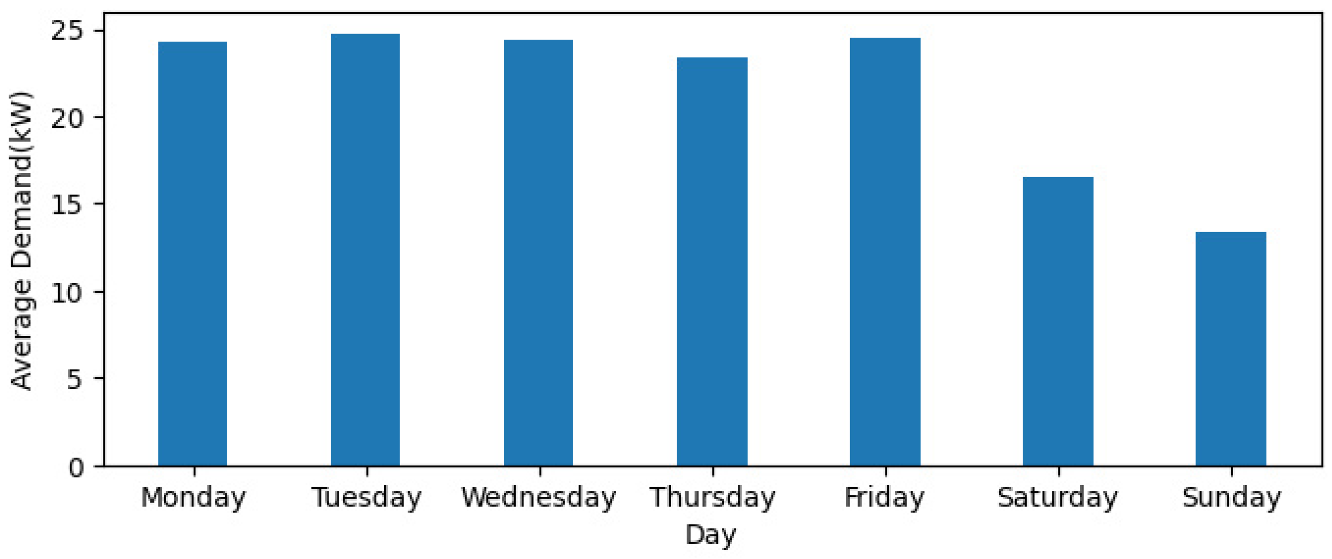
3.2.2. Data Analysis
3.2.3. Outliers Removal
3.2.4. Normalization
3.3. Feature Addition, Correlation Analysis, and Feature Selection
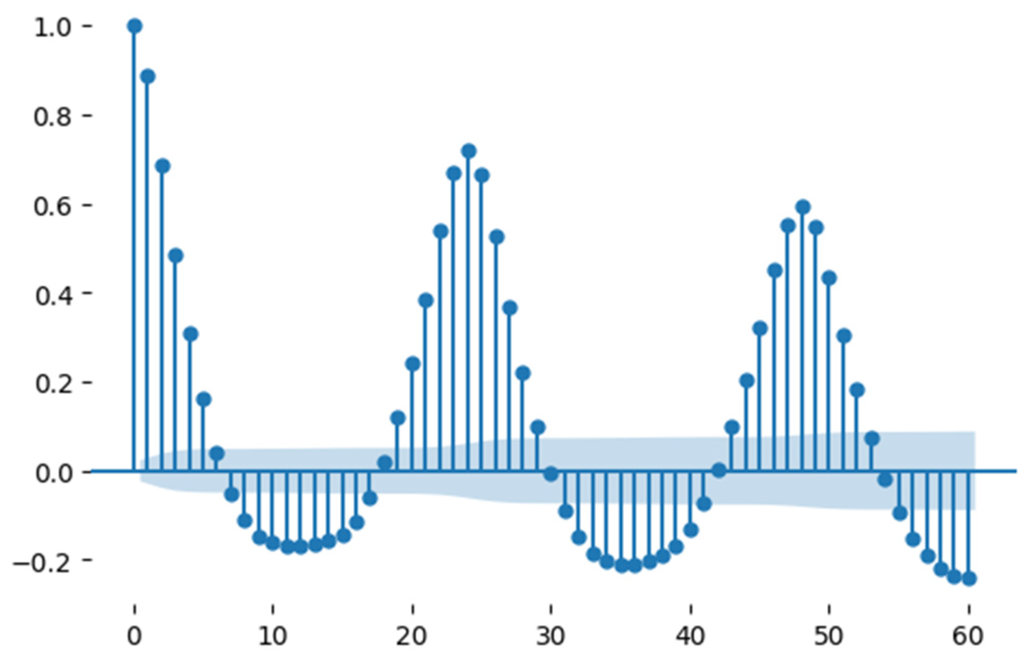
3.3.1. Autocorrelation Plot
3.3.2. Correlation Matrix
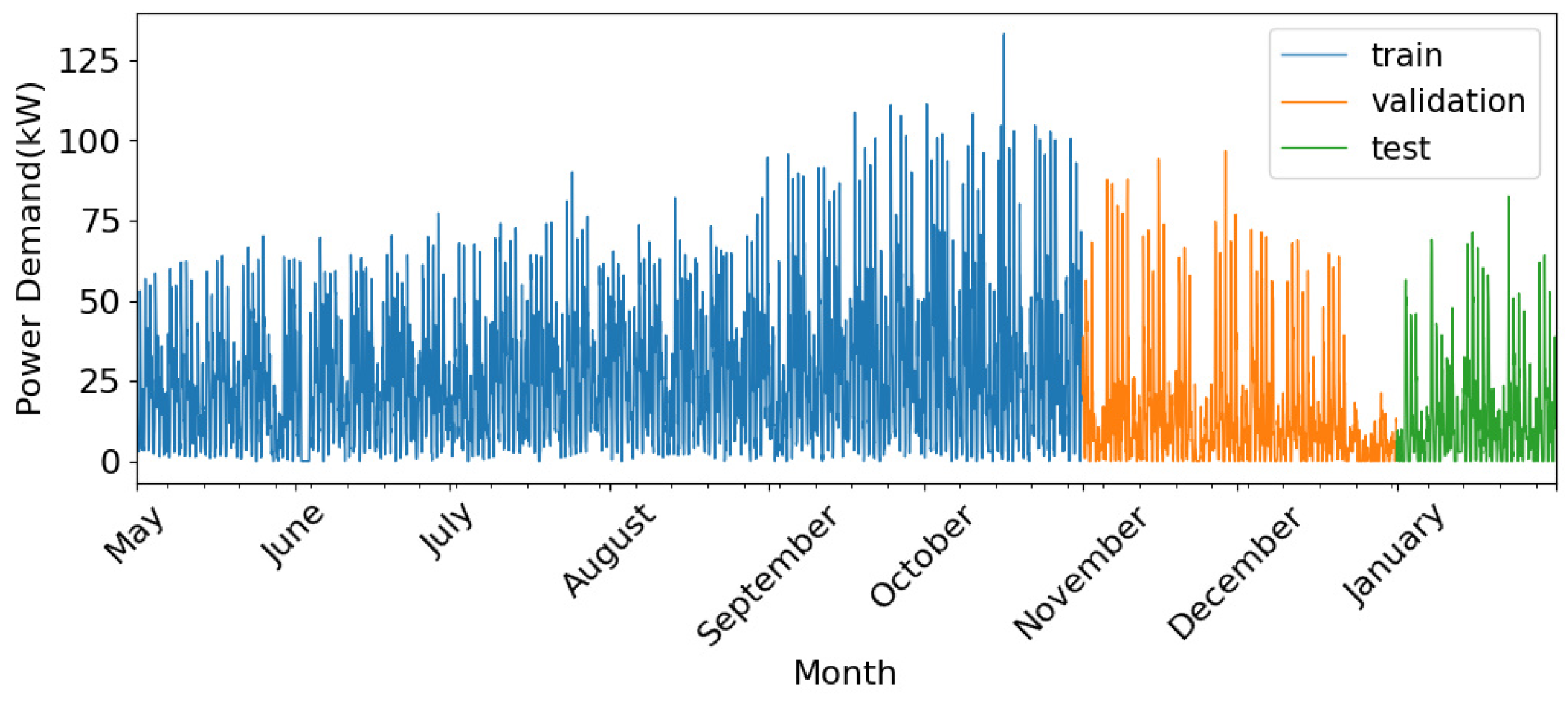
3.3.3. Data Partitioning
3.4. Algorithms and Implementation
3.4.1. Auto-Regressive (AR) and Auto-Regressive Exogenous (ARX) Forecasting
3.4.2. SVR
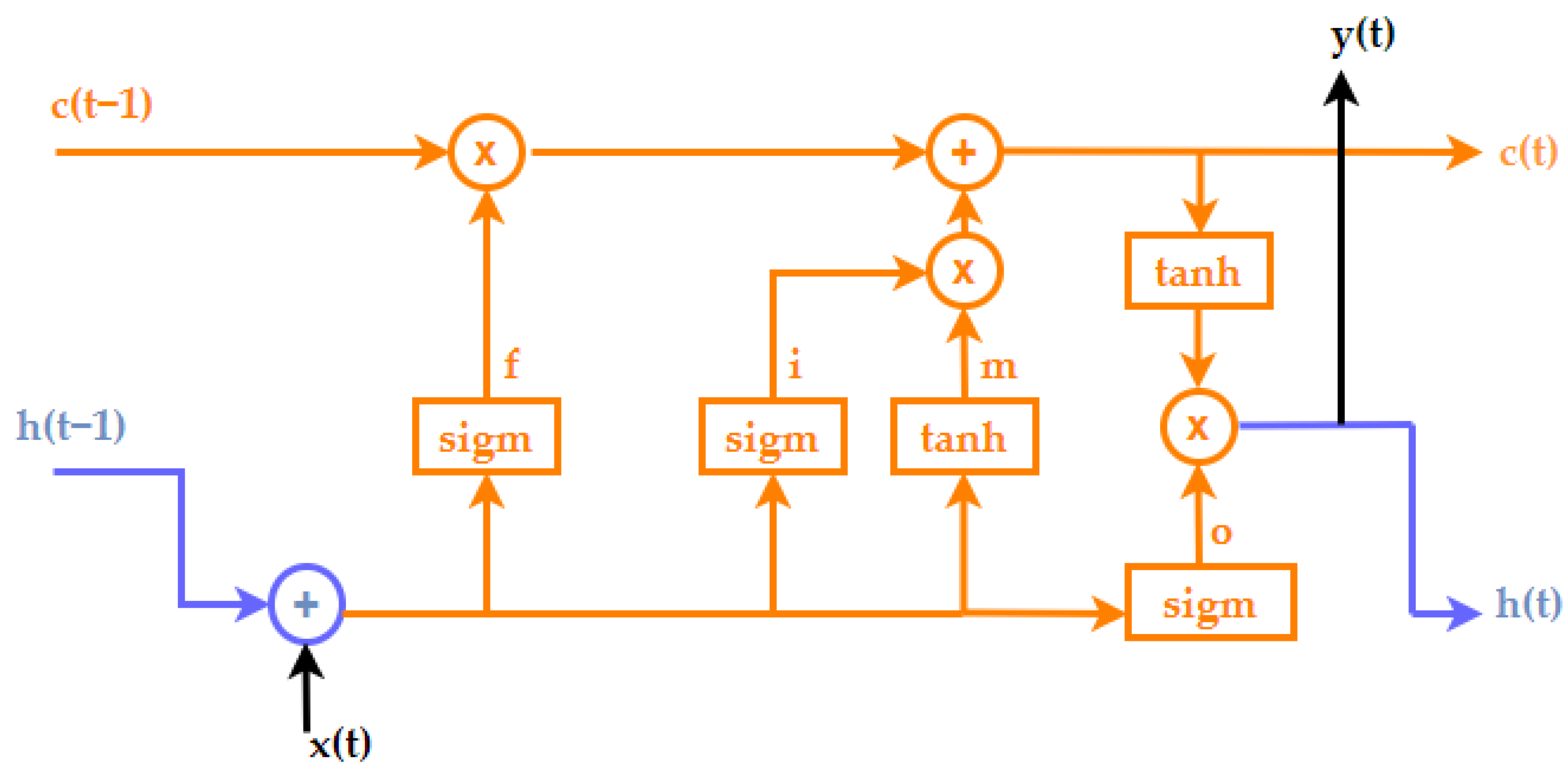
3.4.3. LSTM
3.4.4. Implementation
- (a)
- AR and ARX: The AR model is univariate, considering the target-predicted variable as the only feature. Here, the only feature considered is ‘AggregatedPower’. ForecasterAutoreg class in sklearn package is used to implement the regression model. Among the various regressors, Ridge regressor is found to present the best performance on the dataset. A lag parameter of 48 is decided, meaning that output at each step depends on the previous 48 steps. ARX is multivariate, where it considers multiple attributes for prediction. The model considers ‘ConnectionHour’, ‘WorkingStatus’, ‘HourlyAverageDemand’, and ‘Previous24HrAverageDemand’ features as exogenous variables along with the target variable ‘AggregatedPower’. The model uses a Ridge regressor and a lag of 48.
- (b)
- SVR: In the SVR model with RBF kernel, the attributes ‘ConnectionHour’, ‘WorkingStatus’, ‘HourlyAverageDemand’, and ‘Previous24HrAverageDemand’ are considered as the independent features and ‘AggregatedPower’ as the target. The best values for hyperparameters are obtained using grid search. Regularization parameter (C) is obtained as ten and gamma as one.
- (c)
- LSTM: Multivariate LSTM model is considered where the features are ‘ConnectionHour’, ‘WorkingStatus’, ‘HourlyAverageDemand’, ‘Previous24HrAverageDemand’, and ‘AggregatedPower’. A step size of 48 is chosen after trial and error, which means, the output power at any step is influenced by the values of these features for the previous 48 steps. Multiple LSTM configurations were tried, and performance was evaluated. Finally, the model having one LSTM layer of 50 neurons and tanh activation, followed by a fully connected layer with 50 neurons and ReLu activation and a single neuron at the output layer, is chosen as the best model. The configurations chosen for the models are given in Table 2.
3.4.5. Performance Metrics
- (a)
- ME:
- (b)
- MAE:
- (c)
- RMSE:
- (d)
- MAPE:
4. Results and Discussions
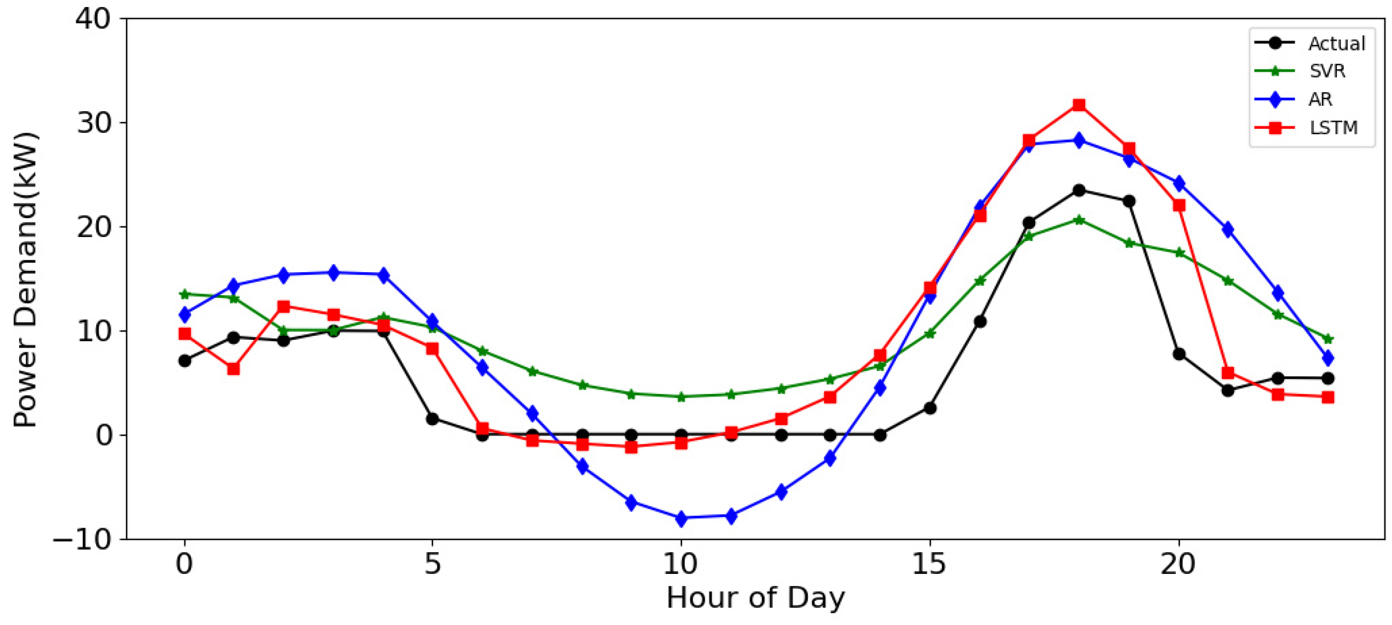
4.1. Prediction on a Normal Weekend
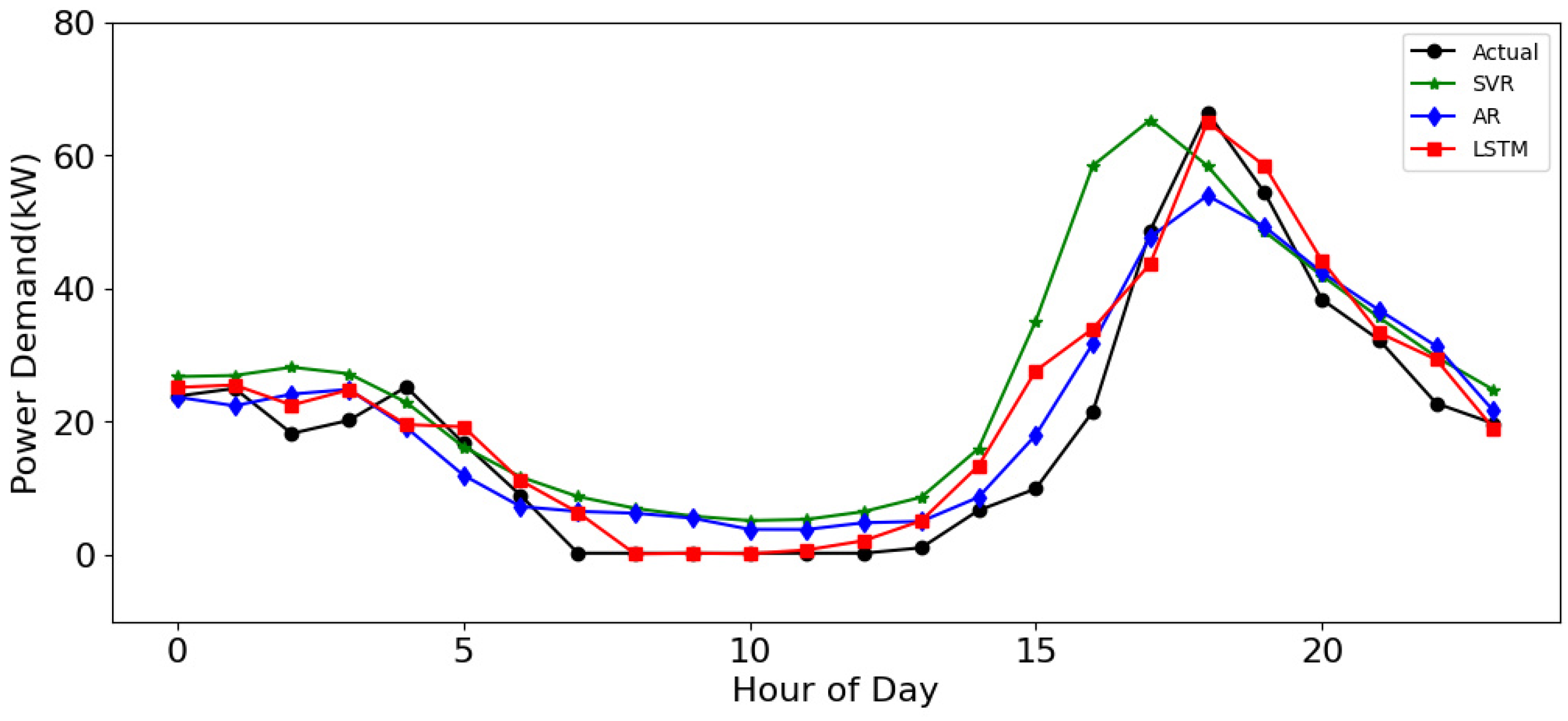
4.2. Prediction on a Normal Weekday
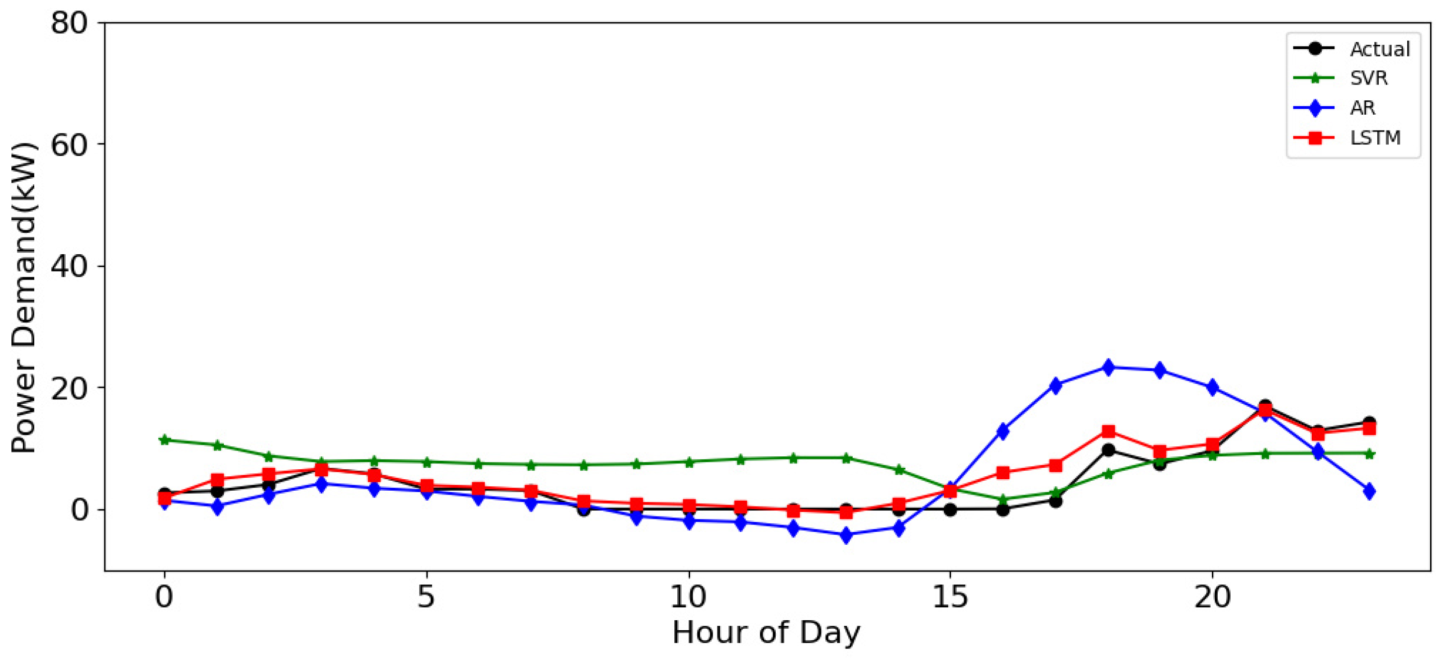
4.3. Prediction on a Weekday Holiday
5. Conclusions and Future Scope of Work
Author Contributions
Funding
Data Availability Statement
Acknowledgments
Conflicts of Interest
References
- Khurana, A.; Kumar, V.V.R.; Sidhpuria, M. A Study on the Adoption of Electric Vehicles in India: The Mediating Role of Attitude. Vis. J. Bus. Perspect. 2019, 24, 23–34. [Google Scholar] [CrossRef]
- Dimitrov, R.S. The Paris Agreement on Climate Change: Behind Closed Doors. Glob. Environ. Politics 2016, 16, 1–11. [Google Scholar] [CrossRef]
- Available online: https://olawebcdn.com/ola-institute/OMI_White_Paper_Vehicle_to_Grid_(V2G)_in_India.pdf (accessed on 13 February 2023).
- Bjerkan, K.Y.; Nørbech, T.E.; Nordtømme, M.E. Incentives for Promoting Battery Electric Vehicle (BEV) Adoption in Norway. Transp. Res. Part D Transp. Environ. 2016, 43, 169–180. [Google Scholar] [CrossRef]
- Song, S.; Lin, H.; Sherman, P.; Yang, X.; Chen, S.; Lu, X.; Lu, T.; Chen, X.; McElroy, M.B. Deep Decarbonization of the Indian Economy: 2050 Prospects for Wind, Solar, and Green Hydrogen. iScience 2022, 25, 104399. [Google Scholar] [CrossRef]
- Bistline, J.E.T.; Young, D.T. The Role of Natural Gas in Reaching Net-Zero Emissions in the Electric Sector. Nat. Commun. 2022, 13, 4743. [Google Scholar] [CrossRef] [PubMed]
- Sortomme, E.; El-Sharkawi, M.A. Optimal Charging Strategies for Unidirectional Vehicle-To-Grid. IEEE Trans. Smart Grid 2011, 2, 131–138. [Google Scholar] [CrossRef]
- Chan, C.C. The State of the Art of Electric, Hybrid, and Fuel Cell Vehicles. Proc. IEEE 2007, 95, 704–718. [Google Scholar] [CrossRef]
- Ehsani, M.; Gao, Y.; Gay, S.E.; Emadi, A. Modern Electric, Hybrid Electric and Fuel Cell Vehicles; CRC Press: Boca Raton, FL, USA, 2004. [Google Scholar]
- Eldho, K.P.; Deepa, K. A comprehensive overview on the current trends and technological challenges in energy storages and charging mechanism in electric vehicle. J. Green Eng. 2020, 10, 9. [Google Scholar]
- Poornesh, K.; Nivya, K.P.; Sireesha, K. A Comparative Study on Electric Vehicle and Internal Combustion Engine Vehicles. In Proceedings of the 2020 International Conference on Smart Electronics and Communication (ICOSEC), Trichy, India, 10–12 September 2020. [Google Scholar] [CrossRef]
- Vempalli, S.K.; Deepa, K. A Novel V2V Charging Method Addressing the Last Mile Connectivity. In Proceedings of the 2018 IEEE International Conference on Power Electronics, Drives and Energy Systems (PEDES), Chennai, India, 18–21 December 2018. [Google Scholar] [CrossRef]
- Wang, Z.; Wang, S. Grid Power Peak Shaving and Valley Filling Using Vehicle-To-Grid Systems. IEEE Trans. Power Deliv. 2013, 28, 1822–1829. [Google Scholar] [CrossRef]
- Yilmaz, M.; Krein, P.T. Review of the Impact of Vehicle-To-Grid Technologies on Distribution Systems and Utility Interfaces. IEEE Trans. Power Electron. 2013, 28, 5673–5689. [Google Scholar] [CrossRef]
- Biresselioglu, M.E.; Demirbag Kaplan, M.; Yilmaz, B.K. Electric Mobility in Europe: A Comprehensive Review of Motivators and Barriers in Decision Making Processes. Transp. Res. Part A Policy Pract. 2018, 109, 1–13. [Google Scholar] [CrossRef]
- Berkeley, N.; Jarvis, D.; Jones, A. Analysing the Take up of Battery Electric Vehicles: An Investigation of Barriers amongst Drivers in the UK. Transp. Res. Part D Transp. Environ. 2018, 63, 466–481. [Google Scholar] [CrossRef]
- Powell, S.; Cezar, G.V.; Min, L.; Azevedo, I.M.L.; Rajagopal, R. Charging Infrastructure Access and Operation to Reduce the Grid Impacts of Deep Electric Vehicle Adoption. Nat. Energy 2022, 7, 1–14. [Google Scholar] [CrossRef]
- Almaghrebi, A. The Impact of PEV User Charging Behavior in Building Public Charging Infrastructure. Master’s Thesis, University of Nebraska-Lincoln, Lincoln, NE, USA, May 2020. [Google Scholar]
- Global Electric Vehicle Market 2020 and Forecasts Canalys Newsroom. Available online: https://canalys.com/newsroom/canalys-global-electric-vehicle-sales-2020 (accessed on 13 February 2023).
- Xydas, E.S.; Marmaras, C.E.; Cipcigan, L.M.; Hassan, A.S.; Jenkins, N. Forecasting Electric Vehicle Charging Demand Using Support Vector Machines. In Proceedings of the 2013 48th International Universities’ Power Engineering Conference (UPEC), Dublin, Ireland, 2–5 September 2013. [Google Scholar] [CrossRef]
- Yusuf, J.; Hasan, J.; Sadrul, U. Impacts of Plug-in Electric Vehicles on a Distribution Level Microgrid. In Proceedings of the 2019 North American Power Symposium (NAPS), Wichita, KS, USA, 13–15 October 2019. [Google Scholar] [CrossRef]
- Yang, Z.; Li, K.; Niu, Q.; Xue, Y. A Comprehensive Study of Economic Unit Commitment of Power Systems Integrating Various Renewable Generations and Plug-in Electric Vehicles. Energy Convers. Manag. 2017, 132, 460–481. [Google Scholar] [CrossRef]
- Hadley, S.W.; Tsvetkova, A.A. Potential Impacts of Plug-in Hybrid Electric Vehicles on Regional Power Generation. Electr. J. 2009, 22, 56–68. [Google Scholar] [CrossRef]
- Brouwer, A.S.; Kuramochi, T.; van den Broek, M.; Faaij, A. Fulfilling the Electricity Demand of Electric Vehicles in the Long Term Future: An Evaluation of Centralized and Decentralized Power Supply Systems. Appl. Energy 2013, 107, 33–51. [Google Scholar] [CrossRef]
- Rahman, S.; Shrestha, G.B. An Investigation into the Impact of Electric Vehicle Load on the Electric Utility Distribution System. IEEE Trans. Power Deliv. 1993, 8, 591–597. [Google Scholar] [CrossRef]
- Gomez, J.C.; Morcos, M.M. Impact of EV Battery Chargers on the Power Quality of Distribution Systems. IEEE Trans. Power Deliv. 2003, 18, 975–981. [Google Scholar] [CrossRef]
- Qian, K.; Zhou, C.; Allan, M.; Yuan, Y. Modeling of Load Demand due to EV Battery Charging in Distribution Systems. IEEE Trans. Power Syst. 2011, 26, 802–810. [Google Scholar] [CrossRef]
- Al-Ogaili, A.S.; Tengku Hashim, T.J.; Rahmat, N.A.; Ramasamy, A.K.; Marsadek, M.B.; Faisal, M.; Hannan, M.A. Review on Scheduling, Clustering, and Forecasting Strategies for Controlling Electric Vehicle Charging: Challenges and Recommendations. IEEE Access 2019, 7, 128353–128371. [Google Scholar] [CrossRef]
- Sharma, I.; Canizares, C.; Bhattacharya, K. Smart Charging of PEVs Penetrating into Residential Distribution Systems. IEEE Trans. Smart Grid 2014, 5, 1196–1209. [Google Scholar] [CrossRef]
- Mohammad; Moses, P.S.; Hajforoosh, S. Distribution Transformer Stress in Smart Grid with Coordinated Charging of Plug-in Electric Vehicles. In Proceedings of the 2012 IEEE PES Innovative Smart Grid Technologies (ISGT), Washington, DC, USA, 16–20 January 2012. [Google Scholar] [CrossRef]
- Richardson, P.; Flynn, D.; Keane, A. Optimal Charging of Electric Vehicles in Low-Voltage Distribution Systems. IEEE Trans. Power Syst. 2012, 27, 268–279. [Google Scholar] [CrossRef]
- Clement-Nyns, K.; Haesen, E.; Driesen, J. The Impact of Charging Plug-in Hybrid Electric Vehicles on a Residential Distribution Grid. IEEE Trans. Power Syst. 2010, 25, 371–380. [Google Scholar] [CrossRef]
- Peng, S.; Zhang, H.; Yang, Y.; Li, B.; Su, S.; Huang, S.; Zheng, G. Spatial-Temporal Dynamic Forecasting of EVs Charging Load Based on DCC-2D. Chin. J. Electr. Eng. 2022, 8, 53–62. [Google Scholar] [CrossRef]
- Bae, S.; Kwasinski, A. Spatial and Temporal Model of Electric Vehicle Charging Demand. IEEE Trans. Smart Grid 2012, 3, 394–403. [Google Scholar] [CrossRef]
- Luo, Z.; Song, Y.; Hu, Z.; Xu, Z.; Yang, X.; Zhan, K. Forecasting Charging Load of Plug-in Electric Vehicles in China. In Proceedings of the 2011 IEEE Power and Energy Society General Meeting, Detroit, MI, USA, 24–28 July 2011. [Google Scholar] [CrossRef]
- Shao, Y.; Mu, Y.; Yu, X.; Dong, X.; Jia, H.; Wu, J.; Zeng, Y. A Spatial-Temporal Charging Load Forecast and Impact Analysis Method for Distribution Network Using EVs-Traffic-Distribution Model. Proc. CSEE Smart Grid 2017, 37, 5207–5219. [Google Scholar] [CrossRef]
- Liang, H.; Sharma, I.; Zhuang, W.; Bhattacharya, K. Plug-in Electric Vehicle Charging Demand Estimation Based on Queueing Network Analysis. In Proceedings of the 2014 IEEE PES General Meeting|Conference & Exposition, National Harbor, MD, USA, 27–31 July 2014. [Google Scholar] [CrossRef]
- Amini, M.H.; Kargarian, A.; Karabasoglu, O. ARIMA-Based Decoupled Time Series Forecasting of Electric Vehicle Charging Demand for Stochastic Power System Operation. Electr. Power Syst. Res. 2016, 140, 378–390. [Google Scholar] [CrossRef]
- Karthick, A.; Mohanavel, V.; Chinnaiyan, V.K.; Karpagam, J.; Baranilingesan, I.; Rajkumar, S. State of Charge Prediction of Battery Management System for Electric Vehicles. In Active Electrical Distribution Network; Academic Press: New York, NY, USA, 2022; pp. 163–180. [Google Scholar]
- Ghosh, A. Possibilities and challenges for the inclusion of the electric vehicle (EV) to reduce the carbon footprint in the transport sector: A review. Energies 2020, 13, 2602. [Google Scholar] [CrossRef]
- Prabha, P.P.; Vanitha, V.; Resmi, R. Wind Speed Forecasting Using Long Short Term Memory Networks. In Proceedings of the 2019 2nd International Conference on Intelligent Computing, Instrumentation and Control Technologies (ICICICT), Kannur, India, 5–6 July 2019. [Google Scholar] [CrossRef]
- Kumar, D.T.S. Video Based Traffic Forecasting Using Convolution Neural Network Model and Transfer Learning Techniques. J. Innov. Image Process. 2020, 2, 128–134. [Google Scholar] [CrossRef]
- Chandran, L.R.; Jayagopal, N.; Lal, L.S.; Narayanan, C.; Deepak, S.; Harikrishnan, V. Residential Load Time Series Forecasting Using ANN and Classical Methods. In Proceedings of the 2021 6th International Conference on Communication and Electronics Systems (ICCES), Coimbatre, India, 8–10 July 2021. [Google Scholar] [CrossRef]
- Arias, M.B.; Bae, S. Electric Vehicle Charging Demand Forecasting Model Based on Big Data Technologies. Appl. Energy 2016, 183, 327–339. [Google Scholar] [CrossRef]
- Chen, W.; Chen, X.; Liao, Y.; Wang, G.; Yao, J.; Chen, K. Short-Term Load Forecasting Based on Time Series Reconstruction and Support Vector Regression. In Proceedings of the 2013 IEEE International Conference of IEEE Region 10 (TENCON 2013), Xi’an, China, 22–25 October 2013. [Google Scholar] [CrossRef]
- Majidpour, M. Time Series Prediction for Electric Vehicle Charging Load and Solar Power Generation in the Context of Smart Grid. Ph.D. Thesis, University of California, Los Angeles, CA, USA, 2016. [Google Scholar]
- Majidpour, M.; Qiu, C.; Chu, P.; Gadh, R.; Pota, H.R. Modified Pattern Sequence-Based Forecasting for Electric Vehicle Charging Stations. OSTI OAI (U.S. Department of Energy Office of Scientific and Technical Information) 2014. In Proceedings of the 2014 IEEE International Conference on Smart Grid Communications (SmartGridComm), Venice, Italy, 3–6 November 2014. [Google Scholar] [CrossRef]
- Almaghrebi, A.; Aljuheshi, F.; Rafaie, M.; James, K.; Alahmad, M. Data-Driven Charging Demand Prediction at Public Charging Stations Using Supervised Machine Learning Regression Methods. Energies 2020, 13, 4231. [Google Scholar] [CrossRef]
- Kandasamy, N.K.; Cheah, P.H.; Sivaneasan, B.; So, P.L.; Wang, D.Z. Electric Vehicle Charging Profile Prediction for Efficient Energy Management in Buildings. In Proceedings of the 2012 10th International Power & Energy Conference (IPEC), Ho Chi Minh City, Vietnam, 12–14 December 2012. [Google Scholar] [CrossRef]
- Aduama, P.; Zhang, Z.; Al-Sumaiti, A.S. Multi-Feature Data Fusion-Based Load Forecasting of Electric Vehicle Charging Stations Using a Deep Learning Model. Energies 2023, 16, 1309. [Google Scholar] [CrossRef]
- Van Kriekinge, G.; De Cauwer, C.; Sapountzoglou, N.; Coosemans, T.; Messagie, M. Day-Ahead Forecast of Electric Vehicle Charging Demand with Deep Neural Networks. World Electr. Veh. J. 2021, 12, 178. [Google Scholar] [CrossRef]
- Elahe, F.; Kabir, A.; Mahmud, S.; Azim, R. Factors Impacting Short-Term Load Forecasting of Charging Station to Electric Vehicle. Electronics 2022, 12, 55. [Google Scholar] [CrossRef]
- Koohfar, S.; Woldemariam, W.; Kumar, A. Prediction of Electric Vehicles Charging Demand: A Transformer-Based Deep Learning Approach. Sustainability 2023, 15, 2105. [Google Scholar] [CrossRef]
- Li, Y.; Huang, Y.; Zhang, M. Short-Term Load Forecasting for Electric Vehicle Charging Station Based on Niche Immunity Lion Algorithm and Convolutional Neural Network. Energies 2018, 11, 1253. [Google Scholar] [CrossRef]
- Wang, J.; Wang, J.; Li, Y.; Zhu, S.; Zhao, J. Techniques of Applying Wavelet De-Noising into a Combined Model for Short-Term Load Forecasting. International J. Electr. Power Energy Syst. 2014, 62, 816–824. [Google Scholar] [CrossRef]
- Wang, J.-Z.; Wang, J.-J.; Zhang, Z.-G.; Guo, S.-P. Forecasting Stock Indices with Back Propagation Neural Network. Expert Syst. Appl. 2011, 38, 14346–14355. [Google Scholar] [CrossRef]
- Gao, Y.; Guo, S.; Ren, J.; Zhao, Z.; Ehsan, A.; Zheng, Y. An Electric Bus Power Consumption Model and Optimization of Charging Scheduling Concerning Multi-External Factors. Energies 2018, 11, 2060. [Google Scholar] [CrossRef]
- Zhang, L.; Huang, C.; Yu, H. Study of Charging Station Short-Term Load Forecast Based on Wavelet Neural Networks for Electric Buses; Springer: Berlin/Heidelberg, Germany, 2014; pp. 555–564. [Google Scholar] [CrossRef]
- Dokur, E.; Erdogan, N.; Kucuksari, S. EV Fleet Charging Load Forecasting Based on Multiple Decomposition with CEEMDAN and Swarm Decomposition. IEEE Access 2022, 10, 62330–62340. [Google Scholar] [CrossRef]
- Lee, Z.J.; Li, T.; Low, S.H. ACN-Data: Analysis and Applications of an Open EV Charging Dataset. In Proceedings of the E-Energy’19: Tenth ACM International Conference on Future Energy Systems, Phoenix, AZ, USA, 25–28 June 2019; California Institute of Technology: Pasadena, CA, USA, 2019. [Google Scholar]
- Mahajan, M.; Kumar, S.; Pant, B.; Tiwari, U. Incremental Outlier Detection in Air Quality Data Using Statistical Methods. In Proceedings of the 2020 International Conference on Data Analytics for Business and Industry: Way Towards a Sustainable Economy (ICDABI), Sakheer, Bahrain, 26–27 October 2020. [Google Scholar] [CrossRef]
- Otexts.com. Available online: https://otexts.com/fpp2/AR.html (accessed on 13 February 2023).
- Horner, M.; Pakzad, S.N.; Gulgec, N.S. Parameter Estimation of Autoregressive-Exogenous and Autoregressive Models Subject to Missing Data Using Expectation Maximization. Front. Built Environ. 2019, 5, 109. [Google Scholar] [CrossRef]
- Boser, B.E.; Guyon, I.M.; Vapnik, V.N. A Training Algorithm for Optimal Margin Classifiers. In Proceedings of the Fifth Annual Workshop on Computational Learning Theory–COLT’92, Pittsburgh, PA, USA, 27–29 July 1992. [Google Scholar] [CrossRef]
- Hsu, C.W.; Chang, C.C.; Lin, C.J. A Practical Guide to Support Vector Classification; Technical Report; Department of Computer Science, National Taiwan University: Taipei, Taiwan, 2016. [Google Scholar]
- Hochreiter, S. The Vanishing Gradient Problem during Learning Recurrent Neural Nets and Problem Solutions. Int. J. Uncertain. Fuzziness Knowl. Based Syst. 1998, 6, 107–116. [Google Scholar] [CrossRef]


| Feature | Description |
|---|---|
| ConnectionHour | Hour of the day at which the vehicle is connected to the charging port |
| DayofWeek | Day number e.g., 0—Sunday, 1—Monday |
| Week | Week number of the year |
| WorkingStatus | Binary value, indicating working day or holiday: 1 for working day, 0 for holiday |
| HourlyAverageDemand | Average power demand for the given connection hour |
| Previous24HrAverageDemand | Average demand for the previous 24 h |
| AggregatedPower | EV charging demand (kW) |
| Model | Parameter | Value |
|---|---|---|
| ARF | Regressor | Ridge |
| Lags | 48 | |
| Kernel | RBF | |
| SVR | C | 10 |
| Gamma | 1 | |
| Epochs | 30 | |
| LSTM | Batch Size | 192 |
| Optimizer | Adam | |
| Learning Rate | 0.001 | |
| Output Activation Function | Linear |
| Performance Metric | AR | ARX | SVR | LSTM |
|---|---|---|---|---|
| ME (kW) | 63.2 | 42 | 43 | 24 |
| MAE (kW) | 8.5 | 7.4 | 7.7 | 4.2 |
| RMSE (kW) | 12.6 | 10.1 | 10.5 | 5.9 |
| MAPE * | 0.73 | 0.86 | 0.71 | 0.4 |
Disclaimer/Publisher’s Note: The statements, opinions and data contained in all publications are solely those of the individual author(s) and contributor(s) and not of MDPI and/or the editor(s). MDPI and/or the editor(s) disclaim responsibility for any injury to people or property resulting from any ideas, methods, instructions or products referred to in the content. |
© 2023 by the authors. Licensee MDPI, Basel, Switzerland. This article is an open access article distributed under the terms and conditions of the Creative Commons Attribution (CC BY) license (https://creativecommons.org/licenses/by/4.0/).
Share and Cite
Vishnu, G.; Kaliyaperumal, D.; Pati, P.B.; Karthick, A.; Subbanna, N.; Ghosh, A. Short-Term Forecasting of Electric Vehicle Load Using Time Series, Machine Learning, and Deep Learning Techniques. World Electr. Veh. J. 2023, 14, 266. https://doi.org/10.3390/wevj14090266
Vishnu G, Kaliyaperumal D, Pati PB, Karthick A, Subbanna N, Ghosh A. Short-Term Forecasting of Electric Vehicle Load Using Time Series, Machine Learning, and Deep Learning Techniques. World Electric Vehicle Journal. 2023; 14(9):266. https://doi.org/10.3390/wevj14090266
Chicago/Turabian StyleVishnu, Gayathry, Deepa Kaliyaperumal, Peeta Basa Pati, Alagar Karthick, Nagesh Subbanna, and Aritra Ghosh. 2023. "Short-Term Forecasting of Electric Vehicle Load Using Time Series, Machine Learning, and Deep Learning Techniques" World Electric Vehicle Journal 14, no. 9: 266. https://doi.org/10.3390/wevj14090266
APA StyleVishnu, G., Kaliyaperumal, D., Pati, P. B., Karthick, A., Subbanna, N., & Ghosh, A. (2023). Short-Term Forecasting of Electric Vehicle Load Using Time Series, Machine Learning, and Deep Learning Techniques. World Electric Vehicle Journal, 14(9), 266. https://doi.org/10.3390/wevj14090266