Article

State of Health Estimation for Lithium-Ion Batteries Using IAO–SVR

1
College of Electrical and Information Engineering, Anhui University of Science and Technology, Huainan 232001, China
2
School of Mechanical and Electrical Engineering, Huainan Normal University, Huainan 232038, China
*
Author to whom correspondence should be addressed.
World Electr. Veh. J. 2023, 14(5), 122; https://doi.org/10.3390/wevj14050122
Submission received: 11 April 2023 / Revised: 30 April 2023 / Accepted: 3 May 2023 / Published: 7 May 2023

Abstract

:
The state of health (SOH) of lithium-ion batteries (LIBs) needs to be accurately estimated to ensure the safety and stability of electric vehicles (EVs) while in operation. In this paper, we proposed a SOH estimation method based on Improved Aquila Optimizer (IAO) and Support Vector Regression (SVR) to achieve an accurate estimation of SOH. During the charging and discharging phases of the battery, we analyzed the trends in current, voltage, and energy, then extracted four features. We used the Kendall coefficient and gray relational grade to prove that features and SOH were highly correlated. On the other hand, IAO was used to optimize the penalty factor and kernel function parameters of the SVR to further improve the generalization and mapping ability. The proposed method was verified under different operating conditions using the CACLE battery data set; the results show that high accuracy can be achieved in SOH estimation via IAO–SVR, and the estimation error of mean MAE is remaining within 2%.

1. Introduction

Because of the oil crisis and severe pollution, gasoline-fueled automobiles do not follow the path of sustainable development. In addition, as the idea of green, energy-efficient, and low-carbon growth becomes more widespread. EVs have begun to enter the public consciousness. LIBs are widely used as the power source in EVs due to their high energy density, long cycle life, and lack of memory [1,2,3,4]. However, the SOH of the LIBs will change after a long period of usage, and it will influence the performance and safety of LIBs.
During the battery degeneration, the cathode material dissolution releases lithium ions, and the negative electrode material is gradually oxidized [5]. The reasons will result in reduced battery capacity, seriously affecting the accuracy of the state of charge (SOC) [6]. The internal chemical reaction rate decreases, and the internal resistance increases, leading to a decrease in the maximum discharge power and available energy of the battery, the state of energy (SOE), and state of power (SOP) are also affected [7]. More seriously, battery degeneration can lead to environmental changes, with high temperatures and high humidity changes, and the state of safety (SOS) of the battery will change and cause safety accidents [8,9]. Thus, the parameter of SOH needs to be accurately obtained, it could maintain the stable operation of the battery and prevent safety accidents [10,11].
SOH cannot be measured directly. There are many methods for SOH estimation, in general, they can be divided into two categories: model-based predictive methods and data-driven predictive methods [12,13]. In the former method, SOH is estimated by building a degradation model that describes the battery, then combined with a filtering algorithm. There usually are the Kalman Filter (KF) [14], Particle Filter (PF) [15], and Recursive Least Squares Filter (RLSF) [16]. Chen et al. proposed a second-order centered difference particle filter (SCDPF) to solve the particle degeneracy phenomenon in particle filtering. Then, the method achieved an accurate estimation of SOH [17]. Zeng et al. proposed a fuzzy unscented Kalman filtering algorithm (F-UKF) based on an improved circuit model the F-UKF algorithm was the joint estimation of battery state of charge (SOC) and SOH [18]. The accuracy of the battery model is highly influenced by the model-based method, and it is difficult to accurately establish the model due to the complex mechanism of the battery degradation, which greatly limits the application of this type of method in practical situations.
With the development of machine learning, a data-driven method for estimating SOH has grown in popularity. This method does not require a battery degradation model, it only needs to analyze battery degradation data and then extract the appropriate health features to train the model; then, a highly accurate predicted SOH can be obtained [19,20,21]. Li et al. [22] analyzed the NASA dataset and extracted four health features from charge/discharge curves, then combined features with the Improved Antlion method for SOH estimation. However, the feature extracted from the constant voltage (CV) mode shows a negative correlation with SOH; it should be processed before being used as an input. Zhang et al. extracted features from voltage curves and then build the feature engineering; the features were as input of XGBoost to estimate SOH [23]. The complexity of the overall estimation process is increased by the excessive number of feature points. Deng et al. [24] used GRA to evaluate the correlation between health features and SOH. Then, the most suitable feature can be selected. By analyzing the battery’s incremental capacity (IC) curves, several features were obtained. Wen et al. [25] proposed a BP neural network that can forecast the battery’s SOH at various temperatures. For a data-driven method to estimate SOH, firstly, the choice of health features must be reasonable and reflect the degradation of the battery; then, the hyperparameters must be set appropriately to enable the training model to avoid overfitting and improve prediction accuracy [26].
Constant current (CC) mode is the longest phase during the charging and discharging of the battery. This paper analyzes the changes in current, voltage, and energy in CC mode and extracted four characteristic features from the battery experimental data using the CACLE dataset, which are the time of equal voltage drop, time of constant current charging duration, the energy of constant current charging duration, and average discharge voltage. The four health features were verified to be highly correlated with battery degradation by both the Kendall correlation coefficient and gray relational grade. Additionally, using a logistic-sine–cosine method to enrich the initial population of the AO algorithm and perturb the t-distribution of the parameters for each search for superiority. This paper made improvements to the AO algorithm in both ways, enabling the algorithm to have a better global search ability and jump out of the local optimum ability. The IAO algorithm was used to find the optimal parameters for the SVR, making it possible for SVR to achieve higher prediction accuracy. The comparison tests with other algorithms showed that the IAO–SVR method can both improve the estimation accuracy and high robustness, which has obvious advantages.
This paper can be divided into five sections. Section 1 introduces the common methods and recent research for SOH estimation. In Section 2, it introduces the AO algorithm and our ideas for improving it, and then explains the process of how we combined IAO with SVR. In Section 3, it introduces the health features we extract from the CACLE dataset, and then we verified that features can be used to estimate SOH. In Section 4, it introduces the experiments to validate the algorithm. In Section 5, it introduces the future development of the proposed approach and concludes the whole article.

2. IAO–SVR

2.1. Aquila Optimizer

The swarm intelligence algorithm known as the Aquila Optimizer (AO) was put forth by Abualigah in 2021 [27]. The algorithm was motivated by the hunting behavior of Aquila. This method offers great global exploration capability, effective search efficiency, and quick convergence time compared to conventional algorithms. However, it cannot avoid hitting the local optimum such as conventional algorithms. According to Aquila’s hunting behavior, Abualigah gives four methods representing the AO search process. In the first method, Aquila selects their search space via high soar with the vertical stoop ( X 1 ) . In the second method, Aquila explores the search space via contour flight with a short glide ( X 2 ) In the third method, Aquila explores the convergent space via a low flight with a slow descend attack ( X 3 ) . In the fourth method, when Aquila finds its prey, it will walk and grab prey ( X 4 ) .

2.1.1. Expanded Exploration ( X 1 )

In the first method, when Aquila first identifies the area of its prey, it will high soar with the vertical stoop to select the best hunting. This behavior is expressed as follows:
X 1 ( t + 1 ) = X b e s t ( t ) × ( 1 t T ) + ( X M ( t ) X b e s t ( t ) × r a n d ) ,
where X 1 ( t + 1 ) represents the next solution obtained from the first method, X b e s t ( t ) represents the optimal solution until the t th iteration, 1 t / T is used to control the expanded search, X M ( t ) represents the average value of the current solution at the t th iteration, and r a n d is a random number within the range at [ 0 , 1 ] .

2.1.2. Narrow Exploration ( X 2 )

The second method shows when Aquila has located the area of the prey using the first method, it will hover over the prey and prepare to attack. This method is called contour flight with a short glide attack. This behavior is shown as follows:
X 2 ( t + 1 ) = X b e s t ( t ) × L e v y ( D ) + X R ( t ) + ( y x ) × r a n d ,
L e v y ( D ) = s × u × σ v 1 β ,
σ = Γ ( 1 + β ) × sin e ( π β 2 ) Γ ( 1 + β 2 ) × β × 2 ( β 1 2 ) ,
where X 2 ( t + 1 ) represents the next solution generated by the second search method, D is the dimension of the problem, L e v y is the Levy flight distribution function, which is calculated via Equation (3), X R ( t ) is the random solution in the range of [ 1 , N ] at the t th iteration, s is a constant of 0.01, u and v are random values in [ 0 , 1 ] , σ is calculated using Equation (4), and β is a constant of 1.5. y and x indicates that Aquila has a spiral distribution during the search process, they are calculated as follows:
y = r × cos ( θ ) ,
x = r × sin ( θ ) ,
r = r 1 + U × D 1 ,
θ = ω × D 1 + θ 1 ,
where θ 1 is a constant of ( 3 × π ) / 2 , r 1 is a value between [ 1 , 20 ] , U is constant of 0.00565, D 1 is an integer from 1 to the length of the search space, and ω is a constant of 0.005.

2.1.3. Expanded Exploitation ( X 3 )

When Aquila located the prey’s position, it will use the third method to prepare to land and attack prey. Aquila will descend vertically and with a preliminary attack. This behavior is referred to as low flight with a slow descent attack. This behavior is shown as follows:
X 3 ( t + 1 ) = ( X b e s t ( t ) X M ( t ) ) × α r a n d + ( ( U B L B ) × r a n d + L B ) × δ ,
where X 3 ( t + 1 ) represents the next solution generated by the third method. α and δ are the exploitation adjustment parameters, and their range is between [ 0 , 1 ] ; L B and U B represent the lower and upper bounds of the problem.

2.1.4. Narrow Exploitation ( X 4 )

When Aquila approaches the prey, it will use the fourth method to attack the prey. Aquila will adjust its movement based on prey behavior. This method is called walking and grabbing prey. This behavior is expressed as follows:
X 4 ( t + 1 ) = Q F × X b e s t ( t ) ( G 1 × X ( t ) × r a n d ) G 2 × L e v y ( D ) + r a n d ,
Q F ( t ) = t 2 × r a n d 1 ( 1 T ) 2 ,
G 1 = 2 × r a n d 1 ,
G 2 = 2 × ( 1 t T ) ,
where X 4 ( t + 1 ) represents the next solution generated by the fourth method, Q F is a quality function used to balance the search strategy, G 1 represents the different methods used by Aquila to cope with the escape of prey, G 2 represents the decreasing value between [ 0 , 2 ] , and it represents Aquila’s flight slope from the first position to the last position in pursuit of prey.

2.2. Improved Aquila Optimizer

As a swarm intelligence algorithm, the AO algorithm can properly balance exploration and exploitation abilities and has excellent searchability, but it still slips into local optimum when solving multi-peaked problems. In this research, we improve the AO method in two ways through initial population optimization and optimal solution perturbation to improve its global search and local optimum search abilities. The improved AO algorithm will be used to find the optimal parameters for the SVR.

2.2.1. Population Initialization Method by Logistic-Sin–Cos Chaotic Mapping

In the AO algorithm, initial solutions are randomly generated via Equation (14). The solutions have the property of randomness, but they cannot traverse the scope of the problem well, resulting in the initial population, which will miss the optimal solution. In contrast, chaos has the properties of strong ergodicity and randomness, and population initialization can be conducted using chaotic mapping. Compared to the randomly generated initial population, the initial population generated by the chaotic mapping is more diverse, and the initial solutions are more uniformly distributed in the search space, which can effectively prevent the algorithm from falling into local optima and improving the convergence speed.
As one of the most classical chaotic mapping methods, logistics chaotic is widely used in population initialization because of its randomness, ergodicity, and strong divergence. The authors of [28] proposed a cosine-transform-based chaotic system (CTBCS) and applied it to image encryption; the formula is shown in Equation (15). The CTBCS uses two chaotic mappings as seed mappings to generate chaotic mappings with complex dynamic behavior. When using logistic mapping F ( a , x i ) and sine mapping as G ( b , x i ) , the CTBCS can transform to logistics-sine–cosine (LSC) mapping. The LSC equation is shown as Equation (16).
x i = r a n d × ( U B L B ) + L B ;
x i + 1 = cos ( π ( F ( a , x i ) + G ( b , x i ) + β ) ) ;
x i + 1 = cos ( π ( 4 r x i ( 1 x i ) + ( 1 r ) sin ( π x i ) 0.5 ) ) .
LSC mapping is employed as the population initialization approach in this paper. To demonstrate the effect of different initialization methods, the mapping curves generated by Equations (14) and (16) are presented below. For example, both of them are with one-dimensional data in [ 0 , 1 ] for 1000 iterations.
The above Figure 1 illustrates that the LSC mapping curve has better traversal and more uniform distribution within [ 0 , 1 ] , which increases population diversity, and its use in population initialization via the AO algorithm results in a richer and more diverse initial solution space.

2.2.2. Adaptive t-Distribution Variation

The t-distribution is a probability distribution also known as the Student distribution. Because of the freedom parameter t, t distribution has different characteristics. When the parameter t is small, the t-distribution mainly has the properties of a Cauchy distribution, which can make the solution more diverse and increase global search capability. When the parameter is large, the t-distribution shows the characteristics of the Gaussian distribution, which can make the algorithm not fall into partial solutions and accelerate the convergence speed.
To make the AO algorithm converge faster and find the best solution, an adaptive t-distribution strategy is introduced to the AO algorithm. By introducing an adaptive parameter ω , ω is set a large value early in the iteration to increase the diversity of solutions. The solution gradually approaches the optimal solution in the later iteration. ω is set a small value, and it minimizes the impact of new solutions and can fully preserve valid AO algorithm solutions [29]. The formula for a new solution, and ω is shown below:
X n e w t = X b e s t t + ω · T D ( t ) · X b e s t t ,
ω = a + ( b a ) · T t T ,
where T D ( t ) denotes the degree of freedom parameter t, a = 0.1 , b = 1 , and T denotes maximum iteration.

2.2.3. Support Vector Regression

SVR is an extension of Support Vector Machines (SVM) in the field of regression and is commonly used to solve small-sample, non-linear problems. By constructing a hyperplane that maps the input data into a high-dimensional space, SVR makes it possible to achieve accurate predictions [30]. In SOH estimation, the feature data of a battery can be mapped non-linearly, followed by regression estimation in a high-dimensional space to output the predicted SOH data.
There is a sample set S = { ( x i , y i ) , i = 1 , 2 , , N } x i R n , y i R , x i is the i th input feature values, and y i is the output value of the corresponding sample. N is the size of samples, and n is the number of dimensions of the input. SVR uses a non-linear mapping to map low-dimensional data to a high-dimensional space, which is expressed as follows:
f ( x ) = ω · φ ( x ) + b ,
where ω is the weight vector, b is the intercept distance, and φ ( x ) is the non-linear mapping function. If relaxation variables ξ i and ξ i is introduced, the problem of finding ω and b can be described in mathematical as follows:
min R ( ω , b , ξ ) = 1 2 ω 2 + C i n ( ξ i + ξ i ) ,
s . t y i ω · ϕ ( x ) b ε + ξ i , ω · ϕ ( x ) + b y i ε + ξ i , ξ i , ξ i 0 . ,
where ε ( ε > 0 ) is the maximum error allowed in the regression problem, and C is the penalty factor, indicating the greater the penalty for samples with training error greater than ε . When we introduce Lagrange multipliers and kernel function, the above equation can be transformed into the following equation:
f ( x ) = i = 1 N ( α i α i ) K ( x i , x j ) + b ,
where α i and α i are Lagrange operators, x i are the input vectors for training samples, and x j are input vectors for test samples. K ( x i , x j ) is the kernel function. In the SVR model, there usually are three kernel functions: separate linear kernel function, polynomial kernel function, RBF kernel function, and sigmoid kernel function. In this article, RBF kernel functions are chosen to solve the prediction of SOH. Its definition is as follows:
K R B F ( x i , x j ) = exp ( 1 2 σ 2 x i x j 2 ) ,
where σ is the width of the RBF kernel function, the two most important parameters in the SVR model, respectively: the penalty factor C and the kernel function parameter σ ; adjustment of the two parameters will improve the accuracy of the SVR.

2.3. IAO–SVR Model

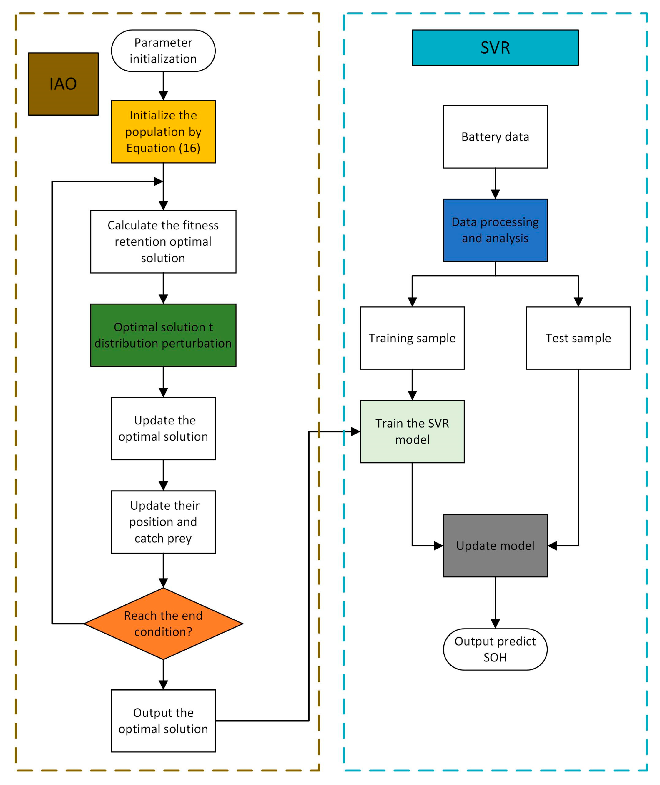
For the SVR to have the best generalization and prediction accuracy, it is necessary to find the best parameters. In the SOH estimation, with the correct C and σ , the estimate can be made as close as possible to the true SOH. In this article, we propose to use an IAO algorithm to find the optimal parameters in the SVR model, coding each parameter pair ( C , σ ) so that they become individual in IAO; then, a suitable fitness function is constructed so that the individual values gradually converge to the optimal values during the training process and find the optimal parameters to obtain the most performance of SVR model. The flowchart of IAO–SVR is shown in Figure 2.
The main steps of IAO–SVR are as follows:
  • Data pre-processing: Sample data is normalized, which allows the pre-processed data to be limited to a certain range, eliminates the influence of abnormal feature vectors, and places each data in the same order of magnitude; then, we can divide the data into training and test samples. The expression is shown in Equation (24) as follows:
    y = y y min y max + y min ,
    where y and y , respectively, are the characteristic values of the sample before and after normalization of the training data, and y min and y max , respectively, are the minimum and maximum values of the sample characteristic data.
  • SVR parameter settings: The SVR parameter settings include the dimension of the individuals D i m , the maximum number of iterations T , the upper bound for individual values U B and lower bound for individual values L B , and the number of populations M a x _ i t e r .
  • Define fitness function: We define the two parameters ( C , σ ) as the individuals of the IAO algorithm; during the training process, each individual will be verified in the SVR. We propose the root mean square error (RMSE) as the fitness function, and the optimal individual is selected by the principle of minimum mean square error as follows:
    R M S E = 1 n i n ( y ^ i y i ) 2 ,
    where y ^ i is the predicted value of the test samples, y i is the actual value of the test samples, and n is the number of test samples.

3. Experiment and Analysis of Health Features

3.1. Definition of SOH

SOH is an important parameter in the battery management system (BMS). It is the ability of a battery to store and release capacity [31]. Understanding the SOH of batteries is important for their maintenance and management. In this article, SOH is expressed in terms of capacity, and it is defined as follows:
S O H = C i C o × 100 % ,
where C i denotes the capacity of the battery in the i th , and C o denotes the nominal capacity of the battery.

3.2. Battery Experiment

Data for this paper comes from the Centre for Advanced Life Cycle Engineering (CACLE) battery degradation experiment at Maryland University [32]. The battery life research uses CX series batteries and CS2 series batteries. Both of them are prismatic cells; their capacities are 1.35 AH and 1.1 AH. The main research of this paper focuses on the CS2 series batteries; the parameters are shown in Table 1.
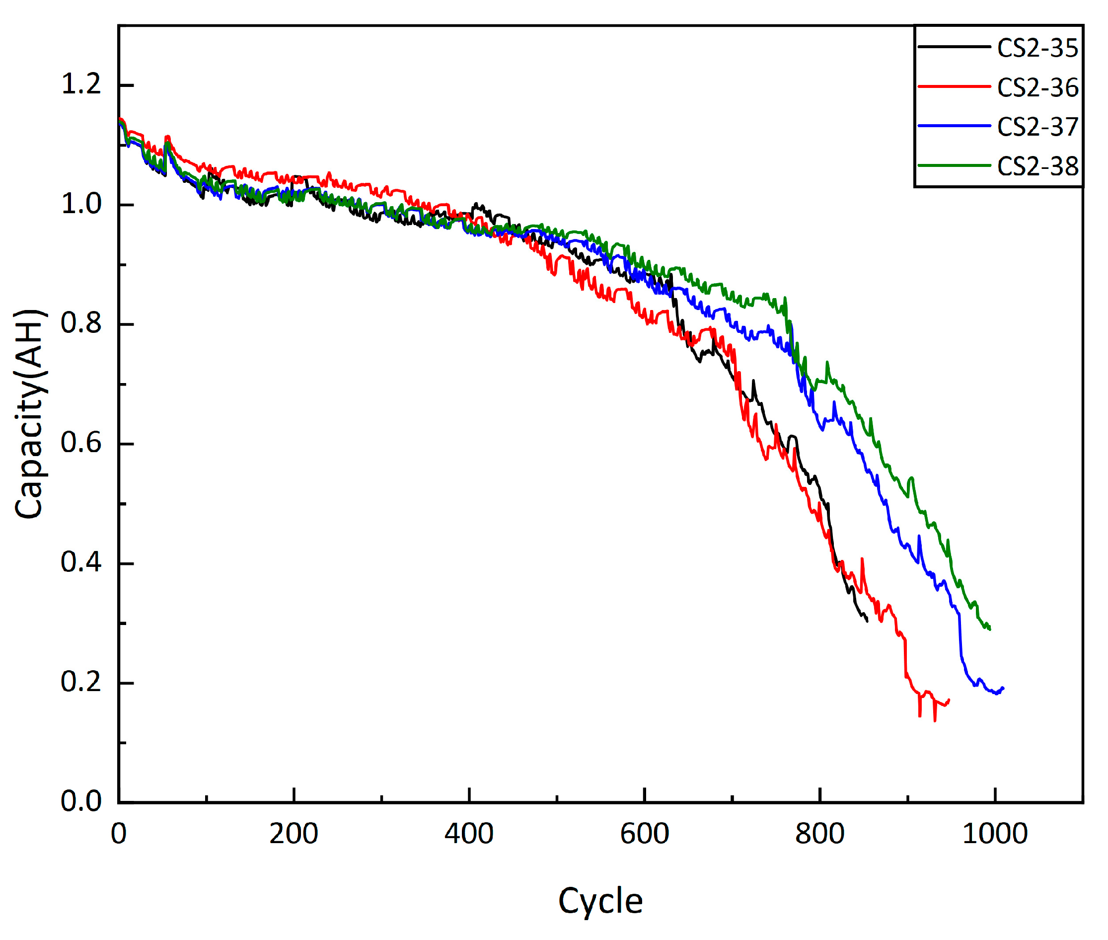
The CS2 series batteries selected for this paper include CS2-35, CS2-36, CS2-37, and CS2-38. All degenerating experiments were carried out at laboratory temperature (20–25 °C), the charge phase is divided into the constant current (CC) part and the constant voltage (CV) part. First, charging at 0.5 C (0.55 A) in a CC mode, when detecting the battery reaches the cut-off voltage (4.2 V), it will turn to a CV mode, and when the current reach to limit current 0.05 C (0.05 A), the whole charge phase end. The discharge phase battery release current at 1 C (1.1 A), and when the battery voltage is detected to be below the cut-off voltage (2.7 V), the discharge is terminated. The experimental environment is shown in Figure 3; it includes four CS2 series batteries, a temperature chamber, a battery test system, and a PC. The temperature chamber is used to control the temperature and maintain a stable range. The test system is possible to implement programmable charge and discharge current, which allows batteries to be aged according to a constant CC–CV protocol. The PC is used to record and store the data during the experiment. Figure 4 shows the battery degradation curve of the CS2 series.
We further analyzed the change in the internal resistance of the battery based on the change in battery capacity. The curve is shown in Figure 5, from which it can be seen that the internal resistance increases as the battery ages and the battery capacity is decreasing. This reflects that the conductive ions in the battery decrease when the charge/discharge cycle and the conductive performance deteriorate, which is consistent with the degradation characteristics of the battery.
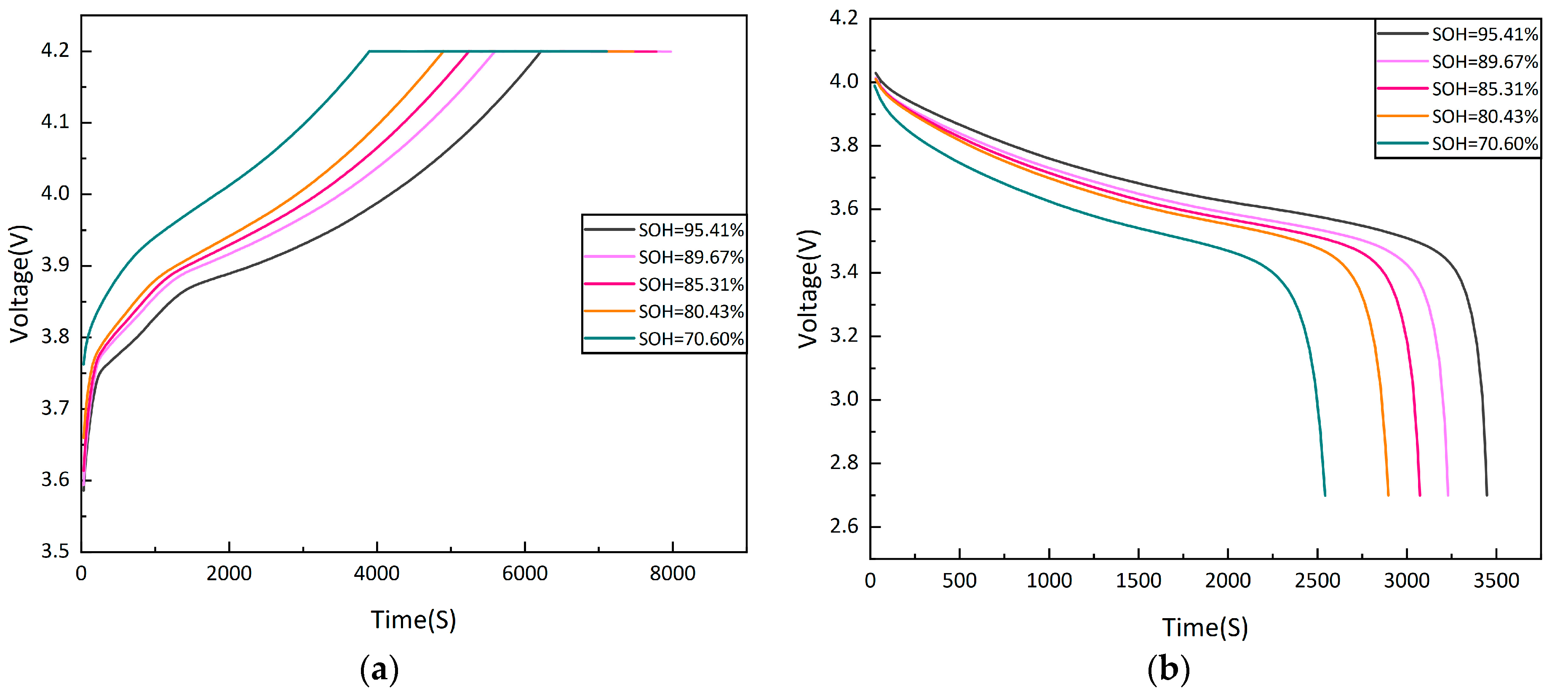
It should be noted that as the battery degradation progresses, the charge and discharge voltages change accordingly. Figure 6a,b show the curve of the charge phase and discharge phase of a battery in different SOH. From Figure 5, it can be seen that the more the battery degradation, the earlier the time at which the constant voltage charge is reached and the faster the battery voltage drops, indicating that the battery is deteriorating.

3.3. Selection of Health Features

By inputting multidimensional feature data, the SVR model enables SOH prediction. Therefore, the selection of feature quantities must be able to accurately describe the variation trend of the SOH. We focused on which data recorded in the experiment would change as a result of battery degradation. As mentioned in Section 1, battery aging leads to a loss of conductive ions, making it easier for the battery to end up in a charged phase and a discharged phase. This results in a CC–CV charging phase and a CC discharging phase; it only takes less time to complete the whole process. In Section 1, it also introduces that with battery aging, batteries have a reduced ability to store and release energy, and SOE will decrease. Thus, the initial health features extracted from the previous analysis of the battery data are as follows.
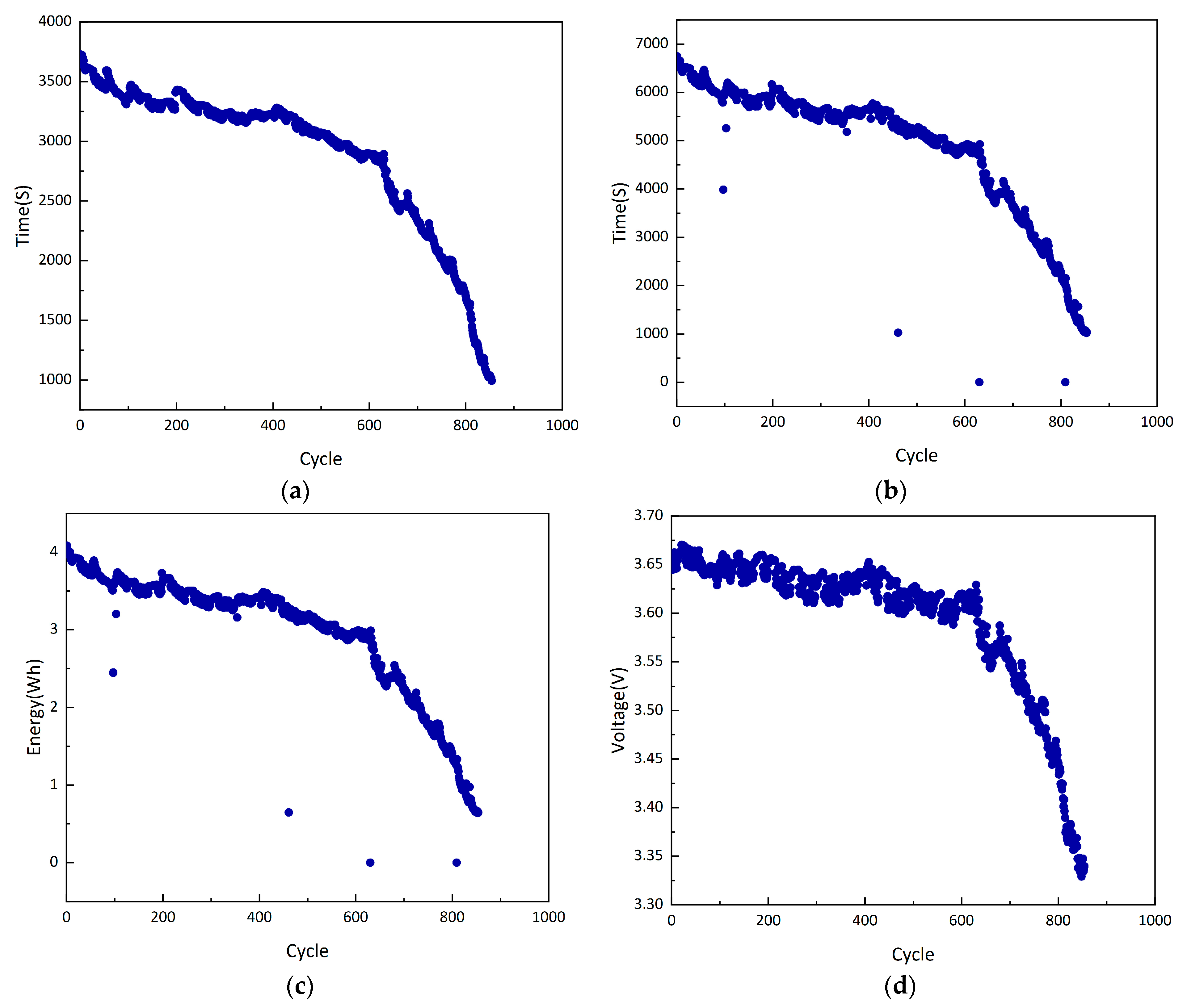
F1: Time of equal voltage drop. From Figure 7a, the voltage gradually drops from 4.2 V to 2.7 V. Within the same voltage drop range, the time gradually decreases, which reflects the battery has reduced electrical conductivity in line with its aging characteristics.
F2: Time of constant current charging duration. From Figure 7b, battery charging time in constant current mode, which gradually decreases when the cycle times increase, is the response to the reduction in available capacity.
F3: Energy of constant current charging duration. From Figure 7c, the charge energy required by the battery in the constant current mode decreases when the cycle times increase; it is due to battery degradation and increased polarization.
F4: Average discharge voltage. From Figure 7d, when averaging the discharge voltage in each cycle, the variation curve of the voltage is the same as SOH, which can be used as a health feature.
For the example of the CS2-35 battery, Figure 7 shows the four health features of this battery. To ensure that the health features are able to accurately describe the degradation characteristics of the battery. We will further analyze the correlation between these health features and the SOH of the battery.

3.4. Correlation Analysis

In this part, we analyze the relationship between health features and battery degradation. Kendall’s correlation coefficient was used to quantify SOH and health features. As a general non-parametric approach, it is less sensitive to outliers and more tolerant. First, the following definition is proposed: two sets, X and Y , both having N elements, and two random variables taking the i th value are denoted by X and Y , respectively, which are called a set of element pairs containing the elements of ( X i , Y i ) When any two elements ( X i , Y i ) in the collection are in the same rank as ( X j , Y j ) , the two elements are considered consistent ( X i > X j , and   Y i > Y i , or   X i < X j , and   Y i < Y i ) . Otherwise, they are considered inconsistent. The Kendall correlation coefficient is calculated as follows:
τ = C D 1 2 N ( N 1 ) ,
where C is the number of elements with consistency in X and Y , and D represents the number of element logarithms with inconsistency. In this article, X is the health characters, and Y is the SOH.
In this paper, GRA is introduced as a tool to verify the correlations and also to improve the rationality of the selected health features. GRA is an active branch of grey system theory, which uses the degree of similarity in the geometry of the series curves to determine whether the relationships are strong or not. Its calculation steps are as follows:
(1)
Set the reference sequence x 0 and the comparison sequence x i ;
(2)
Pre-process the variables to simplify calculations by reducing the range of variables;
(3)
Calculate the correlation coefficient between the comparison series and the reference series, where it is a constant value and ρ is taken as 0.5. The specific formula is expressed as follows:
y ( x 0 ( k ) , x i ( k ) ) = min ( i ) min ( k ) x 0 ( k ) x i ( k ) + ρ max ( i ) max ( k ) x 0 ( k ) x i ( k ) x 0 ( k ) x i ( k ) + ρ max ( i ) max ( k ) x 0 ( k ) x i ( k ) .
The gray relational grade is obtained by averaging the values obtained from Equation (28) using the following formula:
γ = 1 n i = 1 n y ( i ) .
Figure 8 shows the correlation between the health features and SOH, verified by the Kendall coefficient and gray relational grade. The closer the correlation coefficient is to 1, the stronger the correlation. When the correlation coefficient is greater than 0.8, it illustrates that health features are highly correlated with SOH, and as seen from the figure, all four health factors have correlation coefficients greater than 0.8 using Kendall’s method. The gray relational grade of F1, F2, and F3 are greater than 0.8; only F4 is less than 0.8, but it is still very close to 0.8. So, the health features reasonably describe SOH, and they can be used as inputs to the SVR.

4. The SOH Estimation and Result Analysis

4.1. Experimental Environment

We developed experiments on MATLAB 2020B, and battery data come from the CACLE of Maryland University. Four health features were used as inputs to the SVR model, 70% of samples were used for training, with the remaining 30% used for testing. SOH estimation was conducted with SVR’s non-linear mapping capability. AO–SVR, SSA–SVR, and SVR were used as experimental control groups to verify the validity of IAO–SVR.

4.2. Analysis of Estimation Results

To quantitatively analyze the performance of different methods. Three error evaluation criteria are proposed for the evaluation of the merits of algorithms, namely coefficient of determination ( R 2 ) , mean absolute error (MAE), and RMSE. Table 2 specifically shows the error evaluation criteria for SOH estimation using the four methods.
From Table 2, it can be seen that the IAO–SVR method is significantly better than the AO–SVR, SSA–SVR, and SVR methods in the four sets of experiments performed on the batteries. When comparing the four groups of batteries, we can understand that the R 2 of the IAO–SVR method is the closest to 1, which also shows that the IAO–SVR method has the best fit and is closest to the true SOH curve. The mean value of the MAE obtained by IAO–SVR is 0.71%, which is almost two times smaller than the AO–SVR method of 1.40%, which is also much smaller than the SVR method of 2.42%. The mean value of the RMSE obtained via IAO–SVR is 0.95%, and the AO–SVR method is similar to SSA–SVR, which are 1.86% and 1.88%, respectively. The three methods are better than the SVR method at 3.46%.
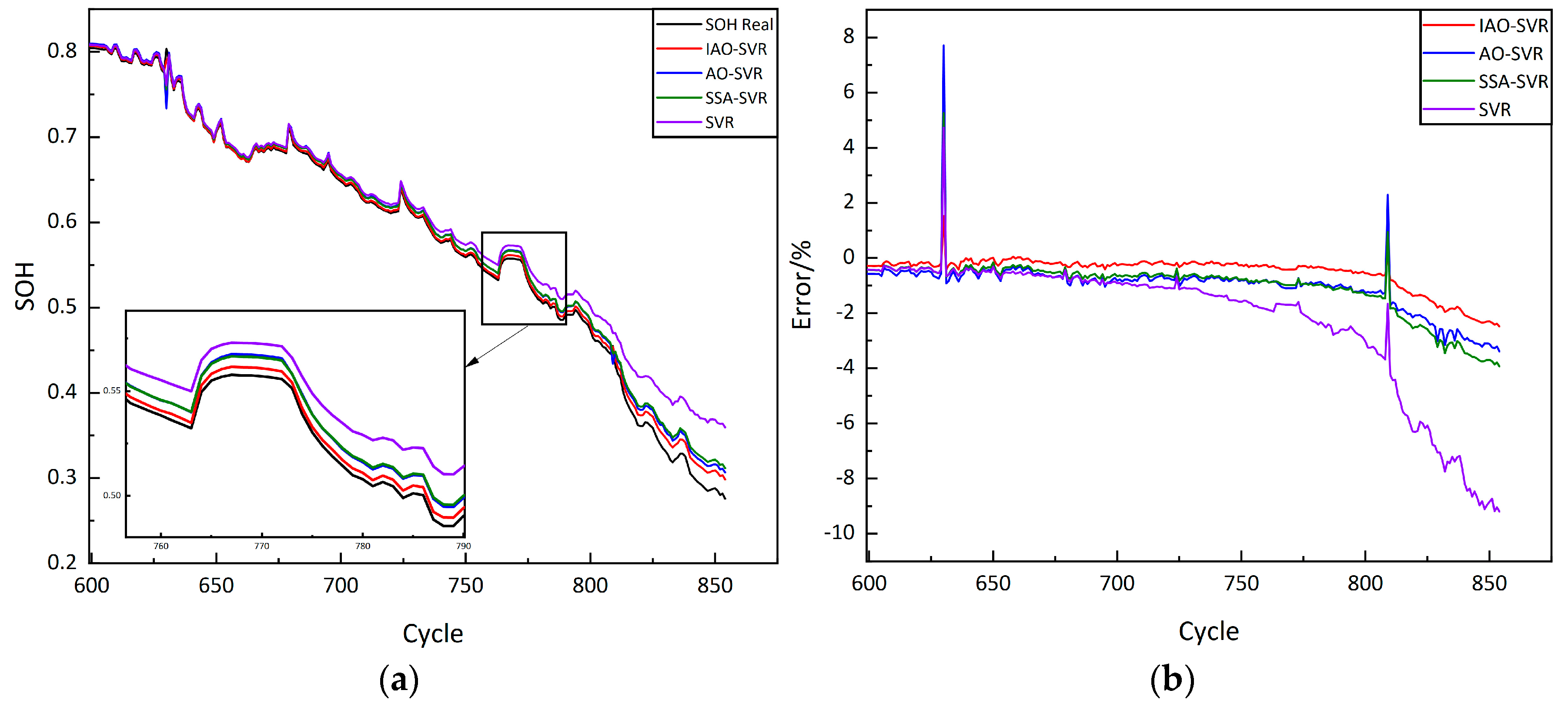
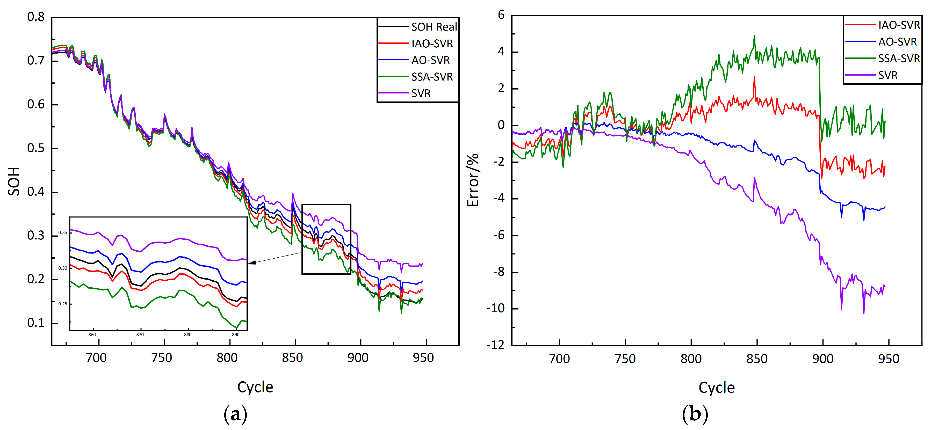
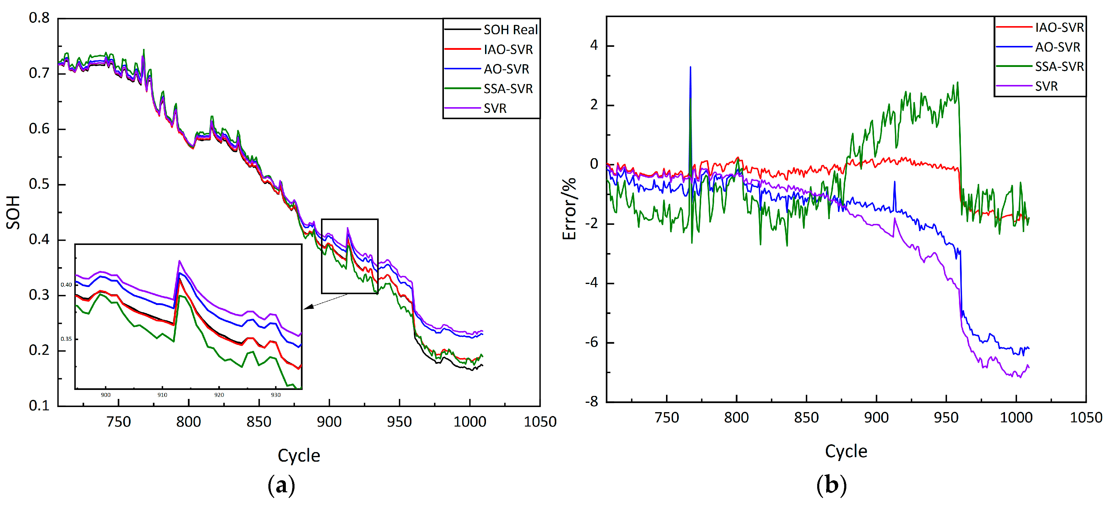
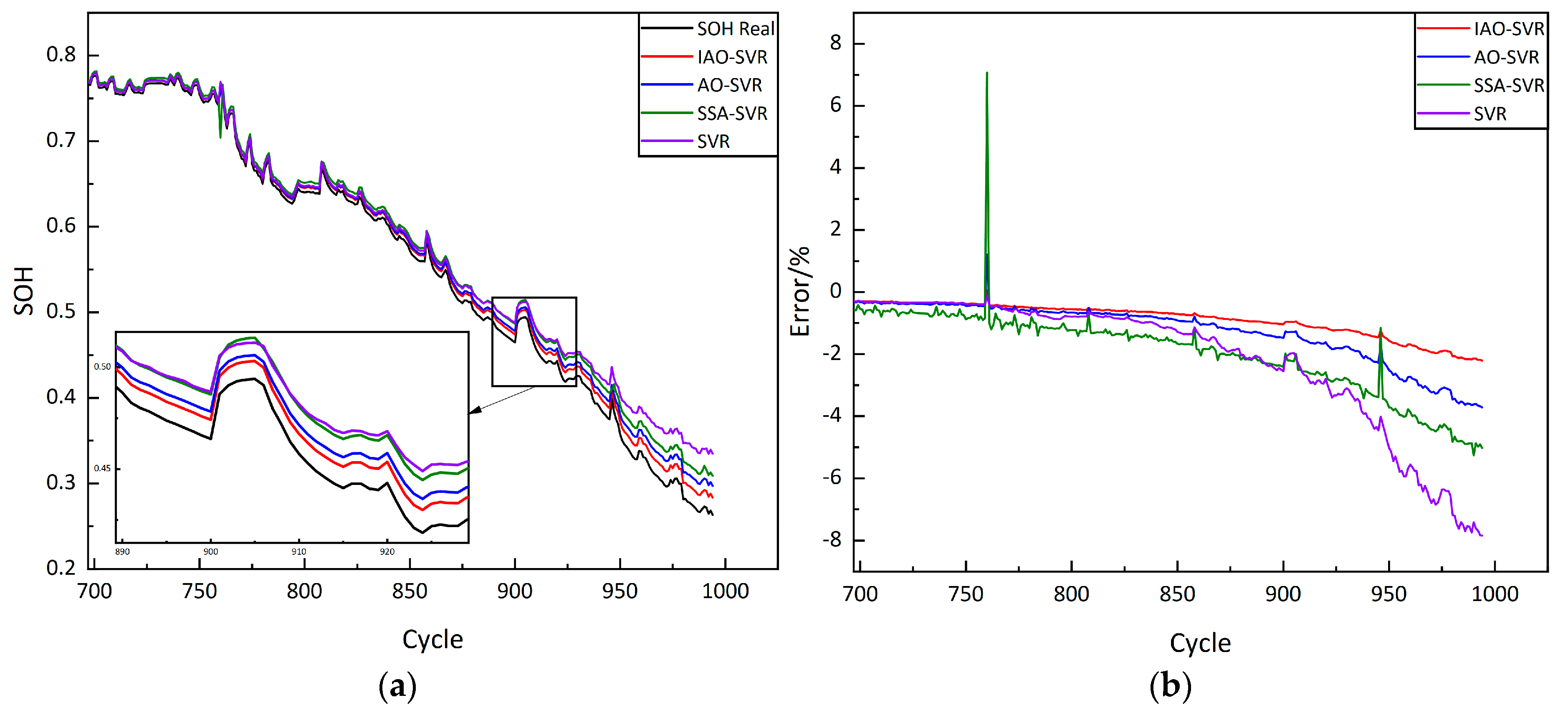
It can be concluded that the proposed IAO–SVR method is more suitable for estimating SOH. The IAO method can improve the predictive power and generalize the SVR model to a large extent. Additionally, we can conclude that from the mean MAE value and the mean RMSE, in the estimation of SOH, AO–SVR retains less error compared to SSA–SVR. To visually demonstrate the comparison of the four methods, the following Figure 9, Figure 10, Figure 11 and Figure 12 show the prediction set estimation curves with errors for the four batteries.
It can be visually observed from the above figure that IAO–SVR can have accurate SOH estimation compared to the other methods. For batteries with a smooth SOH decline, CS2-35 and CS2-38 are taken as examples. Figure 9 and Figure 12 show that the error of the IAO–SVR method remains in a very low range, stable within approximately 2%. Additionally, the estimated performances of the AO–SVR and SSA–SVR are similar for both batteries. It can be concluded that the IAO algorithm can find better penalty factors and kernel function parameters that make SVR a better mapping capability and prediction accuracy.
Additionally, for batteries with a rapid drop in SOH due to internal environmental deterioration, CS2-36 and CS2-37 are taken as examples, Figure 10 and Figure 11 show that the IAO–SVR is a good estimate of the true SOH until the SOH drops rapidly. The error in the IAO–SVR method also does not increase dramatically after a rapid drop in SOH. This means that the IAO–SVR method is more advantageous when dealing with heavily aged batteries.
In conclusion, the IAO–SVR method performs better overall than the AO–SVR, SSA–SVR, and SVR for the same input features. The proposed method has higher accuracy and robustness in estimating SOH.

5. Conclusions

This paper proposed an innovative method to estimate the SOH of LIBs. Uncovering hidden information about battery degradation in both the CC charge and CC discharge phases. Using parameters such as voltage and energy as health features to describe battery degradation. The correlation between the features and SOH was verified by combining Kendall coefficients and GRA coefficients. The results show that the features were highly responsive to the degradation of the batteries The IAO algorithm was used to solve the problem of low prediction accuracy due to poor selection of SVR parameters. After comparative experiments on the validation of the data set based on CACLE, it is shown that the proposed IAO–SVR method can greatly improve the predictive and generalization ability of SVR. Comparative experiments with four groups of batteries show that the error range of IAO–SVR could be kept within a relatively small range, with the maximum of MAE and RMSE of IAO–SVR within 1% for all batteries, and the maximum error of IAO–SVR is around 2%. Therefore, the IAO–SVR can do a better job for SOH estimation, which has significant implications for the study of battery degeneration.

Author Contributions

Conceptualization, X.L.; methodology, X.L.; software, X.L.; project administration, L.X.; resources, L.X. and W.L.; validation, W.L.; visualization, L.W.; data curation, L.X.; writing—original draft, X.L.; writing—review and editing, X.L. and L.X. All authors have read and agreed to the published version of the manuscript.

Funding

This research was funded by the Natural Science Foundation of the Higher Education Institute of Anhui Province (grant KJ2019A0106), Major Research and Development Programs of Huainan City 2021 (grant 2021A249).

Institutional Review Board Statement

Not applicable.

Informed Consent Statement

Not applicable.

Data Availability Statement

The dataset of this manuscript form: https://web.calce.umd.edu/batteries/index.html (accessed on 21 November 2022).

Acknowledgments

The authors thank the Natural Science Foundation of the Higher Education Institute of Anhui Province for helpful discussions on topics related to this work. The authors thank Research and Development Program Projects of Huainan for helpful discussions on topics related to this work. The authors thank the CACLE Data Center for providing the necessary datasets for use in this study.

Conflicts of Interest

The funders had no role in the design of this study; in the collection, analyses, or interpretation of data; in the writing of the manuscript; or in the decision to publish the results.

References

  1. Yao, L.; Xu, S.; Tang, A.; Zhou, F.; Hou, J.; Xiao, Y.; Fu, Z. A review of lithium-ion battery state of health estimation and prediction methods. World Electr. Veh. J. 2021, 12, 113. [Google Scholar] [CrossRef]
  2. Ghalkhani, M.; Habibi, S. Review of the Li-Ion Battery, Thermal Management, and AI-Based Battery Management System for EV Application. Energies 2023, 16, 185. [Google Scholar] [CrossRef]
  3. Yang, S.; Zhang, C.; Jiang, J.; Zhang, W.; Zhang, L.; Wang, Y. Review on state-of-health of lithium-ion batteries: Characterizations, estimations and applications. J. Clean. Prod. 2021, 314, 128015. [Google Scholar] [CrossRef]
  4. Li, J.; Adewuyi, K.; Lotfi, N.; Landers, R.G.; Park, J. A single particle model with chemical/mechanical degradation physics for lithium ion battery State of Health (SOH) estimation. Appl. Energy 2018, 212, 1178–1190. [Google Scholar] [CrossRef]
  5. Golla-Schindler, U.; Zeibig, D.; Prickler, L.; Behn, S.; Bernthaler, T.; Schneider, G. Characterization of degeneration phenomena in lithium-ion batteries by combined microscopic techniques. Micron 2018, 113, 10–19. [Google Scholar] [CrossRef] [PubMed]
  6. Li, S.; Li, K.; Xiao, E.; Xiao, E.; Wong, C.-K. Joint SoC and SoH estimation for zinc-nickel single-flow batteries. IEEE Trans. Ind. Electron. 2020, 67, 8484–8494. [Google Scholar] [CrossRef]
  7. Hu, X.; Feng, F.; Liu, K.; Zhang, L.; Xie, J.; Liu, B. State estimation for advanced battery management: Key challenges and future trends. Renew. Sustain. Energy Rev. 2019, 114, 109334. [Google Scholar] [CrossRef]
  8. Feng, H. An Online Prediction System of Lithium-ion Battery Safety. In Proceedings of the 2021 IEEE International Conference on Advances in Electrical Engineering and Computer Applications, AEECA 2021, Dalian, China, 27–28 August 2021; pp. 399–404. [Google Scholar]
  9. Oji, T.; Zhou, Y.; Ci, S.; Kang, F.; Chen, X.; Liu, X. Data-Driven Methods for Battery SOH Estimation: Survey and a Critical Analysis. IEEE Access 2021, 9, 126903–126916. [Google Scholar] [CrossRef]
  10. Li, C.; Xiao, F.; Fan, Y.; Yang, G.; Tang, X. An Approach to Lithium-Ion Battery SOH Estimation Based on Convolutional Neural Network SOH. Diangong Jishu Xuebao/Trans. China Electrotech. Soc. 2020, 35, 4106–4119. [Google Scholar]
  11. Lin, M.; Yan, C.; Zeng, X. State of Health Estimation Method for Lithium-Ion Batteries via Generalized Additivity Model and Transfer Component Analysis. World Electr. Veh. J. 2023, 14, 14. [Google Scholar] [CrossRef]
  12. Shen, S.; Liu, B.; Zhang, K.; Ci, S. Toward Fast and Accurate SOH Prediction for Lithium-Ion Batteries. IEEE Trans. Energy Convers. 2021, 36, 2036–2046. [Google Scholar] [CrossRef]
  13. Li, J.; Li, Y.; Chen, G.; Lyu, C.; Wu, Y.; Xu, L.; Ma, S. Research on Feature Extraction and SOH Evaluation Methods for Retired Power Battery. Zhongguo Dianji Gongcheng Xuebao/Proc. Chin. Soc. Electr. Eng. 2022, 42, 1332–1346. [Google Scholar]
  14. Bustos, R.; Gadsden, S.A.; Malysz, P.; Al-Shabi, M.; Mahmud, S. Health Monitoring of Lithium-Ion Batteries Using Dual Filters. Energies 2022, 15, 2230. [Google Scholar] [CrossRef]
  15. Wu, T.; Liu, S.; Wang, Z.; Huang, Y. SOC and SOH Joint Estimation of Lithium-Ion Battery Based on Improved Particle Filter Algorithm. J. Electr. Eng. Technol. 2022, 17, 307–317. [Google Scholar] [CrossRef]
  16. Wei, J.; Chen, C. State of Charge and Health Estimation for Lithium-Ion Batteries Using Recursive Least Squares. In Proceedings of the 5th IEEE International Conference on Advanced Robotics and Mechatronics, ICARM 2020, Shenzhen, China, 18–21 December 2020; pp. 686–689. [Google Scholar]
  17. Chen, Y.; He, Y.; Li, Z.; Chen, L.; Zhang, C. Remaining useful life prediction and state of health diagnosis of lithium-ion battery based on second-order central difference particle filter. IEEE Access 2020, 8, 37305–37313. [Google Scholar] [CrossRef]
  18. Zeng, M.; Zhang, P.; Yang, Y.; Xie, C.; Shi, Y. SOC and SOH joint estimation of the power batteries based on fuzzy unscented Kalman filtering algorithm. Energies 2019, 12, 3122. [Google Scholar] [CrossRef]
  19. Pang, B.; Chen, L.; Dong, Z. Data-Driven Degradation Modeling and SOH Prediction of Li-Ion Batteries. Energies 2022, 15, 5580. [Google Scholar] [CrossRef]
  20. Sun, H.; Sun, J.; Zhao, K.; Wang, L.; Wang, K. Data-Driven ICA-Bi-LSTM-Combined Lithium Battery SOH Estimation. Math. Probl. Eng. 2022, 2022, 1–8. [Google Scholar] [CrossRef]
  21. You, G.-W.; Park, S.; Lee, S. Data-driven SOH prediction for EV batteries. In Proceedings of the 2015 IEEE International Conference on Consumer Electronics, ICCE 2015, Las Vegas, NV, USA, 9–12 January 2015; pp. 577–578. [Google Scholar]
  22. Li, Q.; Li, D.; Zhao, K.; Wang, L.; Wang, K. State of health estimation of lithium-ion battery based on improved ant lion optimization and support vector regression. J. Energy Storage 2022, 50, 104215. [Google Scholar] [CrossRef]
  23. Zhang, M.; Chen, W.; Yin, J.; Feng, T. Lithium Battery Health Factor Extraction Based on Improved DouglasPeucker Algorithm and SOH Prediction Based on XGboost. Energies 2022, 15, 5981. [Google Scholar] [CrossRef]
  24. Deng, Y.; Ying, H.; E, J.; Zhu, H.; Wei, K.; Chen, J.; Zhang, F.; Liao, G. Feature parameter extraction and intelligent estimation of the State-of-Health of lithium-ion batteries. Energy 2019, 176, 91–102. [Google Scholar] [CrossRef]
  25. Wen, J.; Chen, X.; Li, X.; Li, Y. SOH prediction of lithium battery based on IC curve feature and BP neural network. Energy 2022, 261, 125234. [Google Scholar] [CrossRef]
  26. Shen, S.; Sadoughi, M.; Li, M.; Wang, Z.; Hu, C. Deep convolutional neural networks with ensemble learning and transfer learning for capacity estimation of lithium-ion batteries. Appl. Energy 2020, 260, 114296. [Google Scholar] [CrossRef]
  27. Abualigah, L.; Yousri, D.; Abd Elaziz, M.; Ewees, A.A.; Al-qaness, M.A.A.; Gandomi, A.H. Aquila Optimizer: A novel meta-heuristic optimization algorithm. Comput. Ind. Eng. 2021, 157, 107250. [Google Scholar] [CrossRef]
  28. Hua, Z.; Zhou, Y.; Huang, H. Cosine-transform-based chaotic system for image encryption. Inf. Sci. 2019, 480, 403–419. [Google Scholar] [CrossRef]
  29. Mao, Q.; Wang, Y. Adaptive T-distribution seagull optimization algorithm combining improved logistics chaos and Sine-cosine operator. J. Chin. Comput. Syst. 2022, 43, 2271–2277. (In Chinese) [Google Scholar]
  30. Cortes, C.; Vapnik, V. Support-vector networks. Mach. Learn. 1995, 20, 273. [Google Scholar] [CrossRef]
  31. Wang, F.; Zhao, Z.; Zhai, Z.; Shang, Z.; Yan, R.; Chen, X. Explainability-driven model improvement for SOH estimation of lithium-ion battery. Reliab. Eng. Syst. Saf. 2023, 232, 109046. [Google Scholar] [CrossRef]
  32. Xing, Y.; Ma, E.W.M.; Tsui, K.-L.; Pecht, M. An ensemble model for predicting the remaining useful performance of lithium-ion batteries. Microelectron. Reliab. 2013, 53, 811–820. [Google Scholar] [CrossRef]
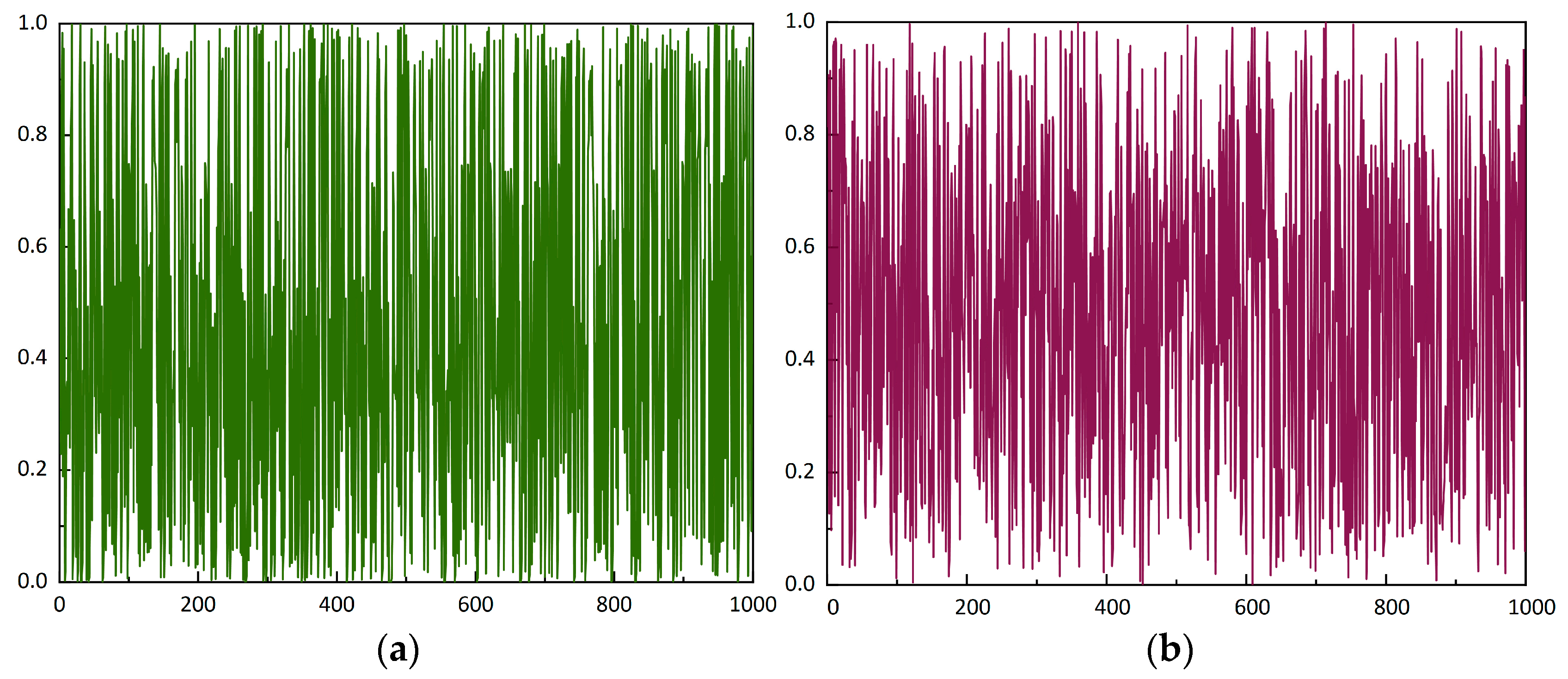
Figure 1. The curves of parameter initializations. (a) Parameter initializes via logistic mapping; (b) Parameter initializes original AO algorithm.
Wevj 14 00122 g001
Figure 2. The flowchart of SOH estimation.
Wevj 14 00122 g002
Figure 3. The battery test environment.
Wevj 14 00122 g003
Figure 4. The curve of battery degeneration.
Wevj 14 00122 g004
Figure 5. The curve of resistance and capacity change of CS2-35.
Wevj 14 00122 g005
Figure 6. The curves of charge voltage and discharge voltage of CS2-35: (a) charge voltage curves; (b) discharge voltage curves.
Wevj 14 00122 g006
Figure 7. The curves of health features: (a) F1, (b) F2, (c) F3, and (d) F4.
Wevj 14 00122 g007
Figure 8. GRA and Kendall correlation coefficient of different health features.
Wevj 14 00122 g008
Figure 9. Prediction results and errors of SOH estimation for CS2-35: (a) Estimation results; (b) Error results.
Wevj 14 00122 g009
Figure 10. Prediction results and errors of SOH estimation for CS2-36: (a) Estimation results; (b) Error results.
Wevj 14 00122 g010
Figure 11. Prediction results and errors of SOH estimation for CS2-37: (a) Estimation results; (b) Error results.
Wevj 14 00122 g011
Figure 12. Prediction results and errors of SOH estimation for CS2-38: (a) Estimation results; (b) Error results.
Wevj 14 00122 g012
Table 1. The parameters of CS2 series batteries.
ParametersSpecifications
ShapePrismatic
Capacity1100 mAH
Weight21.1 g
Dimensions5.4 × 33.6 × 50.6 mm
Table 2. The error criteria of different methods.
BatteryMethod R 2 MAERMSE
CS2-35IAO–SVR0.99760.00520.0081
AO–SVR0.99260.01110.0141
SSA–SVR0.99180.01090.0148
SVR0.97810.02260.0334
CS2-36IAO–SVR0.99600.01030.0124
AO–SVR0.99150.01330.0180
SSA–SVR0.98770.01690.0217
SVR0.95020.03160.0437
CS2-37IAO–SVR0.99870.00420.0071
AO–SVR0.98220.01920.0267
SSA–SVR0.99430.01380.0150
SVR0.97640.02110.0307
CS2-38IAO–SVR0.99650.00880.0102
AO–SVR0.99170.01260.0156
SSA–SVR0.98100.02000.0238
SVR0.96910.02150.0304
Disclaimer/Publisher’s Note: The statements, opinions and data contained in all publications are solely those of the individual author(s) and contributor(s) and not of MDPI and/or the editor(s). MDPI and/or the editor(s) disclaim responsibility for any injury to people or property resulting from any ideas, methods, instructions or products referred to in the content.