Abstract
This paper presents a comprehensive study on autonomous vehicle parking challenges, focusing on kinematic and reverse parking models. The research develops models for various scenarios, including turning, reverse, vertical, and parallel parking while using the minimum turning radius solution. The integration of the A* algorithm enhances trajectory optimization and obstacle avoidance. Innovative concepts like NTBPT and B-spline theory improve computational optimization. This study provides a foundation for understanding the dynamics and constraints of autonomous parking. The proposed model enhances efficiency and safety, reducing algorithm complexity and improving trajectory optimization. This research offers valuable insights and methodologies for addressing autonomous vehicle parking challenges and advocates for advancements in automated parking systems.
1. Introduction
Parking in congested urban areas is a challenge; moreover, non-standard parking can easily cause traffic jams, and the specification of parking, in turn, can help ease urban traffic jams. With the rapid development of automatic driving technology [1,2,3,4,5,6], automatic parking has become a key aspect of automatic driving technology. Moreover, the influence of efficient self-driving car parking is not limited to convenience [7,8,9], improving traffic flow, reducing congestion, and optimizing parking space use. Smooth parking operation helps to improve road safety and reduce accident risk [10,11,12,13,14,15]. Furthermore, automatic parking can potentially reduce fuel consumption, emissions, and parking space requirements. Automatic parking requires vehicles to self-maneuver in the parking space and requires accurate and standardized parking, as well as not to hinder the normal passage of other vehicles, which requires more advanced automatic parking technology.
In a domestic context, researchers have explored various methods of parking in self-driving vehicles [16,17,18]. Some studies have focused on kinematics and reversing parking models using concepts such as the minimum circular arc optimization formula [19,20,21] and the trajectory optimization algorithm A* [21,22,23,24]. These methods are designed to optimize the turning, trajectory, and obstacle avoidance capabilities of autonomous vehicles during parking manipulation. While these methods show promise for improving parking efficiency and safety, their limitations lie in the complexity of the algorithm and the need for accurate sensor data and real-time updates.
Internationally, researchers have also studied innovative technologies for self-driving car parking. These include the integration of machine learning and AI algorithms such as B-spline theory [25,26,27,28,29,30,31] to enhance parking space detection and selection. Reinforcement learning algorithms have been used to train autonomous agents to perform parking tasks effectively. In addition, researchers have explored the use of smart infrastructure, such as smart parking systems and communication technologies [32,33,34,35], to facilitate autonomous car parking. While these approaches offer potential benefits, there are challenges in scalability, infrastructure requirements, and standardized requirements across different regions.
At present, fully autonomous driving has become a reality under various conditions, with industry giants such as Volvo, Mercedes-Benz, Toyota, and Google being at the forefront of developing cutting-edge automation systems [36,37,38,39]. They use advanced technologies such as V2X communications and satellite navigation to constantly improve automatic parking in intelligent transportation systems [40,41]. However, some challenges remain. These measures include ensuring robustness in different real parking lot scenarios through iterative algorithms [42,43,44], addressing complex and dynamic urban environments, and adapting to different parking regulations and cultural norms. In addition, issues of cybersecurity, privacy, and user acceptance of automatic parking systems need to be carefully considered and addressed [43,44,45,46,47].
Among the numerous challenges faced, path-tracking errors during automatic parking remain an obstacle [48,49]. Our study introduces an automated parking path analysis using pre-targeted PID [50,51,52] and a mixed path planning approach based on A * and curve methods to optimize path tracking accuracy [53,54,55]. This improves the safety and efficiency of the automatic parking system and reduces human error during parking, thus improving the utilization of parking spaces and reducing the risks associated with manual parking. This reduces the likelihood of road accidents. Previously, many studies focused on analyzing and optimizing the manufacturing of car components or control systems to improve the quality of components, reduce failure rates, and thereby reduce the likelihood of accidents [56,57,58,59].
As shown in Figure 1, our study helps to advance autonomous vehicle parking systems and address the challenges associated with manipulating and selecting the best parking space. The subsequent sections of this paper present detailed methods and results that demonstrate the effectiveness of our proposed computational optimization model.
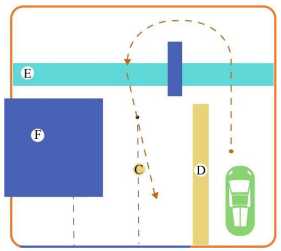
Figure 1.
Parking lot plan with no parking areas.
To facilitate a consideration of the problem, the following assumptions are made in this study while ensuring the accuracy of the model:
- The autonomous vehicle is a symmetrical four-wheeled passenger car with a rectangular body. It adopts front-wheel steering and rear-wheel driving;
- During the vehicle’s motion, the velocity direction at the control point aligns with the direction angle of the trajectory point. The instantaneous turning radius is equal to the curvature radius of the trajectory point;
- The autonomous vehicle travels on an ideal and flat road surface, neglecting any vertical motion of the vehicle;
- Longitudinal and lateral aerodynamic factors are ignored;
- The vehicle acceleration does not exceed 3 m/s2. During the acceleration phase, the constant jerk is assumed to be 20 m/s3;
- All turning maneuvers are assumed to be a constant jerk motion with a circular arc trajectory;
- The maximum centripetal acceleration during a turn is assumed to be equal to the maximum deceleration during braking;
- The time consumed by the friction between the vehicle tires and the ground is negligible;
- Some relevant data of the vehicle included the following: it was 4.9 m long, 1.8 m wide, had a maximum steering wheel angle of 470°, and a steering wheel and front wheel angle of transmission ratio of 16:1 (steering wheel rotation 16°, front wheel rotation 1°).
The description of the symbols in this paper is shown in Table 1.

Table 1.
The description of the symbols.
2. Model Establishment
To better optimize the tracking accuracy, we should first consider constructing a suitable model. The establishment of the model needs to consider two main issues mentioned earlier: one is to solve the problem of the minimum turning radius for unmanned vehicles, and the other is to provide the parking trajectory of unmanned vehicles from their initial position to the designated parking space.
2.1. Unmanned Vehicle Turning Minimum Radius Solving Problem
2.1.1. Solving the Minimum Radius of Unmanned Vehicles
- (1)
- Vehicle steering principle
Modern cars use a technology called Ackermann steering. Prior to the advent of this technology, vehicles (such as horse-drawn carriages) primarily used single-hinged steering technology. Although single-hinged steering also allows the inner and outer steering wheel paths to point to the same circle, it has many disadvantages. Because it has to turn around a single axis in the middle, there is too much room for oscillation, which causes a lot of instability. And because the two front wheels are parallel, they tend to jam when turning excessively and cannot brake.
Ackermann steering technology effectively avoids the disadvantages of single-hinge steering. When the axle turns, the inner and outer wheels turn at different angles, and the inner tire turning radius is smaller than the outer tire. This allows the center of the circle of the four wheels’ paths to meet roughly at the center of the instantaneous steering on the extension of the rear axle, allowing the vehicle to turn smoothly. To specify the Ackermann steering geometry, we denote the wheelbase (the distance from the midpoint of the front axle to the midpoint of the rear axle) as L, the axle length as W, the inner and outer front wheel steering angles as i and o, respectively, and the distance from the vehicle centerline to the instantaneous center of the rotation as R. The formula is as follows [60]:
where is the steering angle of the wheel assumed to be located at the midpoint of the front axle. Taking the inverse of i and tano in the above formula and making the difference, the Ackermann steering formula can be obtained as follows:
- (2)
- Vehicle formulas of motion
The state of the vehicle can be described by (x, y, ϕ, θ).
Specifically, (x, y) denotes the position of the midpoint of the rear axle of the vehicle, θ denotes the body orientation, and φ denotes the front wheel steering angle. To obtain the vehicle motion state based on the front wheel steering φ and the vehicle speed v, the following set of differential formulas are determined:
The instantaneous direction of the motion of the midpoint of the rear axis is perpendicular to the direction of the instantaneous center of the rotation; therefore, the formula is as follows:
The variable v represents the velocity of the vehicle at the midpoint of the rear axle. Next, it is necessary to determine the rotational velocity dθ/dt of the vehicle’s orientation. If we use s to represent the distance traveled by the vehicle (the integral of velocity with respect to time) then we have the following formula: ds = R·dθ. According to the Ackermann steering geometry principle, we know that R = L/tan(ϕ), where R represents the turning radius, L is the wheelbase of the vehicle, and ϕ is the steering angle.
Based on the above analysis, we obtained three differential formulas that describe the motion of the vehicle:
In the established vehicle motion formulas, where v represents the vehicle speed, L represents the wheelbase, and φ represents the front wheel steering angle. According to these formulas, the vehicle’s motion state and trajectory can be reconstructed by performing numerical integration, provided that the control parameters of the vehicle (front wheel steering angle and speed) are known as functions of time. The control parameters, which vary with time, are controlled by the driver: the front wheel steering angle is controlled by the steering wheel, and the vehicle speed is controlled by the throttle and brake.
- (3)
- Vehicle kinematic model
During the parking process, the vehicle’s driving speed is relatively low. Therefore, the lateral slip of wheels during low-speed driving can be ignored. The vehicle can be considered a motion system with non-holonomic constraints. Its kinematic formulas can be expressed as follows:
In the formula: x and y represent the coordinates of the vehicle’s rear axle midpoint along the X and Y axes, respectively. v denotes the velocity of the vehicle at the rear axle midpoint. θ represents the orientation angle of the vehicle’s body. R represents the turning radius at the rear axle midpoint, which is determined by the Ackermann steering geometry principle. The formula is as follows:
R = tan(φ)/L
φ represents the equivalent steering angle at the front axle, and L denotes the wheelbase of the vehicle (as shown in Figure 2).
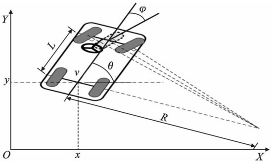
Figure 2.
Ackermann steering geometry principle.
- (4)
- Minimum turning radius solution
Without considering the assumptions, the turning process is illustrated in the following diagram (shown in Figure 3).
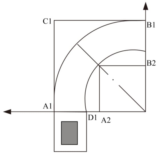
Figure 3.
Ideal state turning simulation.
The formula for calculating the (minimum) turning radius of a vehicle is as follows:
where:
R = L/2(sin φ); D = W + 2R (1 − cos φ)
- R = minimum turning radius of the vehicle (minimum);
- L = vehicle length;
- W = vehicle width;
- D = vehicle minimum turning lane width;
- φ = vehicle direction maximum turning angle; (steering wheel maximum turning angle/16 = 470/16 = 29.375).
By substituting the given values, we can calculate the turning radius as follows:
R = 4.99466 m
2.1.2. Unmanned Vehicles Accelerate in a Straight Line
After solving the minimum turning radius, the acceleration problem of unmanned vehicles traveling in a straight line can be solved.
- (1)
- Modeling.
The initial velocity of the car is v0, the acceleration is , and the acceleration and jerk are .
Therefore, the acceleration at any moment is as follows:
The velocity at any given moment is defined as follows:
The displacement at any given moment is calculated as follows:
Given the following information: .
The objective is to find a solution for the given problem: .
The constraints for the problem are as follows:
We can categorize the problem based on whether the initial acceleration and acceleration and jerk are zero or not.
If the initial acceleration and speed are both zero (a = 0, v = 0), in this scenario, we aim to maximize the value of parameter , which represents the maximum achievable acceleration, to minimize the distance traveled by the vehicle.
- When , we assumed that and the speed is . The route is . The formula is as follows:The solution is: ; .
- When , thereafter, acceleration is , and the acceleration is . Then, the distance is as follows:The result is obtained as follows:
- In other cases, the distance traveled during the acceleration phase can be calculated using the following formula: > 0, > 0, as the maximum value.
2.1.3. Calculation of the Rate of Change of the Relative Path Curvature Length
According to Figure 4, assuming curve C is smooth, the arc on curve C from point B to point B’ is denoted as ΔS, and the tangent angle is denoted as Δα. We define K = |Δα /ΔS| as the average curvature of arc segment MM’. Since we are considering the rate of the change of the relative path length, denoted as Δθ, we have K = |Δθ/ΔS|. In other words, the numerical value of the rate of change Δθ is equivalent to the tangent angle Δα.
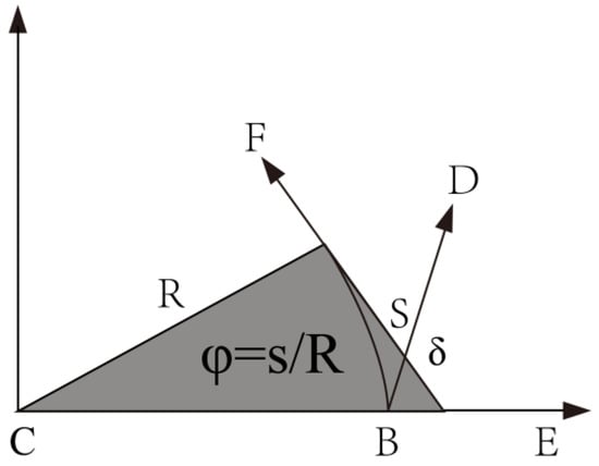
Figure 4.
Curvature relative length change rate calculation.
2.2. Unmanned Vehicle Parking Trajectory
2.2.1. Unmanned Vehicle Reverse Parking Model
In the low-speed reversing range, without considering tire side slip, the trajectory of the rear wheels at any given moment is primarily determined by the wheelbase, track width, and Ackermann steering angle of the front wheel center point. This is independent of the reversing speed of the vehicle, as shown in Figure 5. We can observe that there is a relationship between the steering angle of the front wheels and the trajectory of the rear wheels during the reversing process [61].
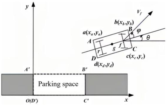
Figure 5.
Kinematic model of the car and diagram of the car position.
In Formula (17), (x0, y) and (xa, ya) represent the coordinates of the contact points a and d of the rear wheels, respectively. L denotes the wheelbase, and Lrw represents the rear wheel track width.
In Figure 5, A′B′C′D′ represents the parking space, ABCD represents the four corners of the vehicle body, and abcd represents the contact points of the four tires. vf denotes the absolute forward speed measured at the front axle center of the vehicle, where positive values indicate forward motion and negative values indicate reverse motion. θ represents the vehicle’s heading angle, with counterclockwise as positive and clockwise as negative. g represents the Ackermann steering angle, with counterclockwise as positive and clockwise as negative.
Based on the above formulas, the trajectory of the vehicle while in reverse can be analyzed. The reverse trajectory is formed by connecting the initial position and the final position of the vehicle using two tangent circular arcs, aiming to simplify the reverse maneuver as much as possible, as shown in Figure 6.
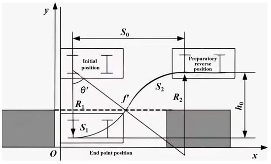
Figure 6.
Simplified diagram of the reversing process.
To simplify the reverse parking model, let us assume that the vehicle has neutral steering, meaning the wheels are not turned during the reverse maneuver. We also restrict the starting and ending positions of the reverse parking to have the same x-coordinate, as shown in Figure 6. By analyzing one complete reverse parking cycle T, we can establish the following model:
The formulas can be obtained by analyzing the specific formulas and conditions of the model:
In these formulas, R1 and R2 represent the turning radii of the right rear wheel of the car when the steering wheel is turned left and right, respectively. S1 and S2 represent the paths traveled by the car when the steering wheel is turned left and right, respectively. S0 and h0 represent the horizontal and vertical distances traveled by the car from the starting position to the destination position. θ′ represents the instantaneous direction angle of the car’s body when it reaches point f′ and begins to reverse the steering wheel.
Next, we analyze the potential collision during the reversing process:
- (1)
- Based on the collision analysis at the vertex D of the vehicle body, the width of the parking space, Sy, is determined. As shown in Figure 7, the radius of the arc covered by the vertex D of the car is calculated as:
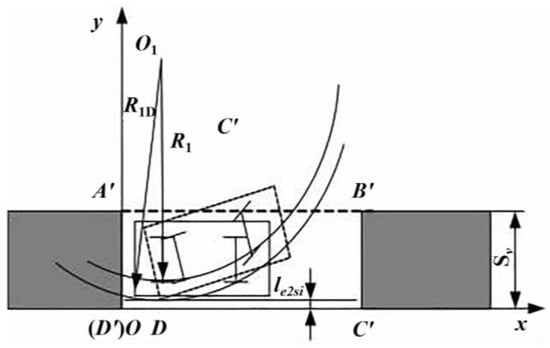 Figure 7. Schematic diagram of the collision analysis between point D of the car body and C′D′ of the parking space.
The minimum extreme value of the parking space width is obtained using:
The width of the parking space is:
As shown in Figure 7, Lrr2r represents the distance from the center plane of the right rear wheel to the right side of the car; Lra2t represents the rear overhang; le2si represents the safety clearance between the right side of the car CD and the inner side C′D′ of the parking space after the successful reverse parking and aligning of the vehicle; W represents the width of the car; δy represents the reserved safety clearance between the car and the parking space in the y-axis direction, obtained using:
δy_outer represents the reserved safety clearance between the outer side of the vehicle and the outer boundary of the parking space in the y-axis direction. For now, let δy_outer = 0.00. δy_inner represents the reserved safety clearance between the right side of the vehicle and the inner part of the parking space in the y-axis direction.
- (2)
- To determine the length Sx of the parking space and the maximum value of R1 based on the potential collision between the vehicle’s vertex C and the parking space’s endpoint B′, the distance between the turning center O1 of the right rear wheel when the steering wheel is turned left and the parking space’s boundary A′B′ is obtained using [62]:
The minimum extremum of the parking space’s length is represented by:
The length of the parking space is obtained using:
As shown in Figure 8, in the formula, Rmin denotes the minimum turning radius of the vehicle; rC2B′ represents the designated safety clearance between the vehicle vertex C and point B′ of the parking space; δx denotes the reserved safety clearance between the vehicle’s rear end and the left side of the parking space, as well as between the vehicle’s front end and the right side of the parking space; L denotes the length of the vehicle.
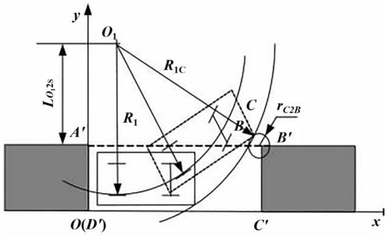
Figure 8.
Schematic diagram of the collision analysis between point C of the car body and point B′ of the parking space.
- (3)
- The minimum value of R2, denoted as R2min, is estimated based on the potential collision between the vehicle vertex B and an obstacle on the other side of the parking space, as shown in Figure 9. The radius of the curvature of the arc covered by the vehicle vertex B is obtained using:
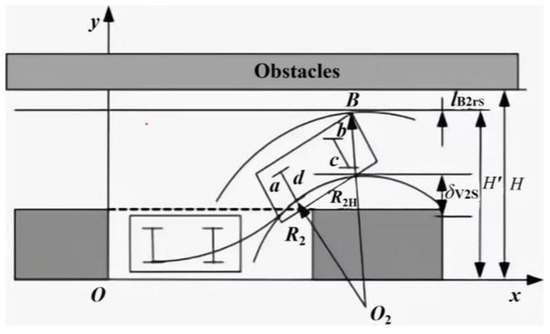 Figure 9. Analysis diagram of the collision between point B of the car and the obstacle on the other side of the parking space.
The required width of the parking space for reverse parking is obtained using:
As shown in Figure 9, H is the width of the reverse parking space; the setup of the parking space does not affect the normal driving of the vehicle. Simultaneously, it ensures convenient entry and exit of the vehicle within the parking space, and it is estimated that H = 6 m.
- (4)
- As shown in Figure 10, based on the analysis of potential collisions between the extended line of the wheel contact point ad and the right side of the vehicle body at point e and the parking space, the maximum value of R2, denoted as R2max, can be determined according to Figure 11. The following formula can be derived:
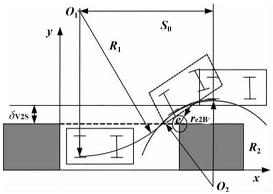 Figure 10. Schematic diagram of the collision analysis between point e of the car body and point B′ of the parking space.
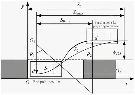 Figure 11. Prepare to reverse the area part of the schematic.
Based on the range of values for R1 and Formulas (8)–(31), the maximum value of R2, denoted as R2max, can be determined.
Finally, the preliminary reverse area of the autonomous vehicle can be determined by defining the ranges of R1 and R2 values. The coordinates of the starting and ending positions of the right rear wheel contact point d, as shown in Figure 12, can be expressed as follows:
Starting position coordinates (xd0, yd0) = (xa− R1 × cos(g + δ), ya − R1 × sin(g + δ)).
Ending position coordinates (xd0, yd0) = (xa − R2 × cos(g − δ), ya − R2 × sin(g − δ)).
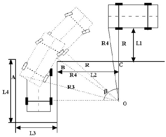
Figure 12.
Vertical parking collision point diagram.
Here, (xa, ya) represents the coordinates of the rear wheel contact point a, R1 and R2 are the turning radii of the right rear wheel, g is the Ackermann steering angle, and δ is the predetermined safety gap.
By determining the ranges of the R1 and R2 values, the corresponding ranges of the starting and ending position coordinates can be calculated, thereby determining the preliminary reverse area of the autonomous vehicle.
In the above formulas, (xd0, yd0) and (xds, yds) represent the coordinates of the right rear wheel contact point d when the vehicle is located at the preliminary reverse position and the endpoint position, respectively. The determined preliminary reverse area has a fixed vertical coordinate. However, as shown in Figure 11, to increase the size of the preliminary reverse area and facilitate the search for a reverse position, the value of the gap δv2s between the vehicle’s body and the parking space at the preliminary reverse position can be adjusted (increased or decreased). This adjustment will change the initial vertical coordinate of the vehicle’s parking position. Then, based on the previously described method, the values of R1 and R2 can be re-determined, thereby expanding the preliminary reverse area of the vehicle.
2.2.2. Unmanned Vehicle Vertical Parking Space Parking Model
In the case of perpendicular parking, a simpler approach can be adopted where the parking is completed in one maneuver by inputting a certain steering wheel angle. This reduces the steps involved in the parking process. The vehicle moves from having 0° between the body and the horizontal plane to 90°, and, then, it is vertically maneuvered into the parking space, as shown in Figure 13. After completing the parking, β = 90°. During this process, collisions may occur at points A and B.
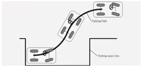
Figure 13.
Parking path tracking.
The collision that occurs at point B is similar to the collision that may occur during parallel parking. The collision at point A involves the left rear part of the vehicle colliding with the left side obstacle of the parking space. The trajectory of this collision has a radius of R, as analyzed below [63]:
The width of the parking space can be obtained using:
The length of the parking space is defined as:
When parking using the minimum turning radius, the minimum parking space width, denoted as L3, is determined. At the same time, the nearest starting position for parking is obtained. The definition of the initial parking area is the same as in parallel parking. Considering the reverse motion of the vehicle coming out of the garage, after avoiding collision points A and B, a larger radius of curvature than Rmin is used to achieve a new starting position for parking. It is also possible to use a radius of curvature larger than Rmin for both maneuvers. However, in this case, as shown in Figure 12, the starting parking position will be farther away from the horizontal obstacle in the vertical direction, and the vehicle’s entry into the parking space will be shallower. This requires a larger space on the left side of the vehicle.
The process of parking in a perpendicular parking space can be divided into five stages. Assuming a maximum speed of 2.78 m/s during the turning phase, we can calculate the time duration for the first stage, denoted as t1. The subsequent stages include uniform acceleration, constant velocity, and deceleration until reaching a complete stop, denoted as t2. The reverse parking stage can be calculated to obtain the time duration, denoted as t3. Finally, the total time for this parking process can be obtained by summing up the durations of each stage:
- (1)
- Steering system
- (2)
- Uniform acceleration and uniform linear travelUniform acceleration:Uniform linear:
- (3)
- Slow down and reverse parking
negative acceleration motion:
2.2.3. Unmanned Vehicle Parking Path Model
- (1)
- Parking path tracking control law
In the context of automatic parking systems, where the steering angle is a controlled input provided by the system, and the vehicle’s speed is controlled by the driver, which is considered a non-controlled input, it is possible to employ a Non-Time-Based Path Tracking (NTBPT) control law to guide the vehicle along the desired parking path.
The NTBPT control law focuses on tracking the desired trajectory without explicitly considering time as a reference. Instead, it aims to maintain the vehicle’s position and orientation relative to the desired path using feedback control techniques. This approach allows for more flexibility in handling variations in vehicle speed during the parking process (as shown in Figure 13).
By utilizing the NTBPT control law, the automatic parking system can effectively guide the vehicle along the desired parking trajectory, taking into account the controlled steering input and adapting to the driver’s control of the vehicle’s speed.
The NTBPT problem can be described as follows: Given a geometric path , we select a non-time reference variable s that monotonically increases with time. Based on this non-time reference variable, denoted as , we seek a feedback control law. For any given small positive number , there exists a threshold value . When s exceeds , the goal paths and are defined, along with the target positions on these paths. The vehicle’s X-axis coordinate is denoted as , and the mapping of the vehicle’s rear axle midpoint’s X-axis coordinate onto the target path is represented by the Y-axis coordinate . Additionally, represents the orientation angle of the vehicle’s rear axle midpoint’s X-axis coordinate mapped onto the target path.
In summary, the NTBPT problem involves selecting a non-time reference variable, defining goal paths and target positions on these paths, and establishing mappings between the vehicle’s coordinates and the target path. The objective is to design a feedback control law that enables the vehicle to track the desired path accurately based on this non-time reference variable, as shown in Figure 14.
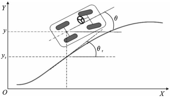
Figure 14.
Path tracking bias.
According to the aforementioned tracking deviation, the path tracking deviation can be represented by Formula (39) as follows:
According to the non-time reference quantity C, the state formula for the non-time reference path tracking deviation can be established as follows [64]:
where represents the curvature of the parking path.
Let be defined as the non-temporal reference for the path tracking deviation. Then, the state formula for the path tracking deviation with respect to -x can be expressed as Formula (42).
The control law for the front wheel equivalent steering angle can be expressed as formula:
The coefficients k1 and k2 in Formula (44) represent the feedback coefficients for the position deviation and heading deviation of the vehicle, respectively.
By choosing k1 > 0 and k2 > 0, according to the first stability theorem of Lyapunov, it can be concluded that the origin is the unique equilibrium point of Formula (45), i.e., the point where the system reaches a stable state [65]:
Based on Formulas (42)–(45), it can be observed that, as the X-axis coordinate of the vehicle’s rear axle midpoint decreases, both the position deviation and heading deviation of the vehicle gradually decrease. This implies that the vehicle is approaching the target path and aligning itself with the desired trajectory.
- (2)
- Parallel parking space parking model
As shown in Figure 15, to parallel park, the process can be divided into 10 stages. Based on Formula (46).Firstly, during the first turning maneuver, the maximum velocity of 2.78 m/s is used to calculate the time t1. Then, the vehicle undergoes uniform acceleration, followed by a period of constant velocity until reaching the second turning point. The time for this stage is calculated as t2. The second turning maneuver takes time t3, and the third turning maneuver takes time t4. Afterward, the vehicle accelerates uniformly and maintains a constant velocity during straight-line driving until finally decelerating to a stop. The time for this straight-line segment is denoted as t5. Lastly, the time for the reverse parking maneuver is calculated as t6. By summing up the individual times, the total time for the parallel parking process can be determined.
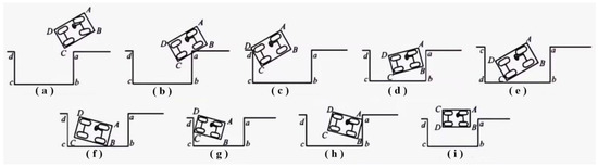
Figure 15.
Collision point studies: (a). Left front-end collision; (b). Right-side collision; (c). Left rear-end collision; (d). Right front-end collision 1; (e). Right rear-end collision 1; (f). Right front-end collision 2; (g). Right rear-end collision 2; (h). Front-end collision; (i). Not fully seated.
- First turn:
- The first straight-line travel:Uniform straight line:Deceleration:
- Second turn:
- Third turn:
- Second straight sectionUniform straight line:
- Slow down and reverse parking:
- Find the total time:22.404 + 1.1 = 23.504 s
- (3)
- Unmanned vehicle 45° inclined parking space parking model
To park in an inclined parking space, the process can be divided into six stages. Firstly, during the first turning maneuver, the maximum velocity of 2.78 m/s is used to calculate the time t1. Then, the vehicle undergoes uniform acceleration, followed by a period of constant velocity until reaching the second turning point. The time for this stage is calculated as t2. After the second turning maneuver, the vehicle maintains a constant velocity and travels a certain distance forward. The time for this segment is denoted as t3. Finally, the time for the reverse parking maneuver is calculated as t4. By summing up the individual times, the total time for the parking process in an inclined parking space can be determined.
Just as in Formula (47), substituting the given data yields the following solution:
3. Problem Solving
Based on the discussion and solution of the above issues, the next step is to apply the model to practical problem applications and solutions.
3.1. Optimal Parking Space Parking Model
Under the assumptions and considerations made in the model, let the speed of the autonomous vehicle during the parking process, whether it is turning or driving straight, be equal to the maximum speed limit of that road segment, denoted as the vehicle.
- (1)
- Parking-oriented analysis
Let us define a coordinate system based on the given n parking positions, denoted as (xi, yi, θi, φi), where:
xi represents the x-coordinate in the direction of the vehicle’s entrance.
yi represents the y-coordinate perpendicular to the entrance.
θi represents the orientation of the autonomous vehicle at the moment before reversing.
φi represents the direction of rotation needed during the reverse parking process, with 0 indicating the positive x-axis direction and values ranging from 0 to 2π for a complete counterclockwise revolution.
We can establish the coordinate system using the entrance of the parking area as the origin and the entrance line as the x-axis. Therefore, the position coordinates of the autonomous vehicle can be represented as (x, y, θ) in this coordinate system.
- (2)
- Curve Analysis
Let the number of curves be Wi, Δθi = θ − θi
The total distance traveled on a curved path can be calculated as S1i = 2πRΔθi, where R is the radius of the curve and Δθi is the angular displacement.
To determine the time required for curved path traversal at a maximum speed v1, we can use the formula:
t1i = S1i/v1
- (3)
- Straight-line path analysis
Let Δxi = x − xi and Δyi = y − yi; then, the distance traveled in a straight line is:
By calculating S1i for each curved path segment, we can determine the time required to traverse them. Let us consider the following speed values:
V2: Speed within 5 m before the deceleration zone.
V3: Speed on other straight sections of the road.
Please note that V1 is the maximum speed for curved paths, V2 is the speed within the 5-m zone, and V3 is the speed on straight sections of the road.
- (A)
- Δθi = 0, time required ti:
- (B)
- Δθi = π/2, time required ti:
- (C)
- Δθi = π, time required ti:
- (4)
- Reversing path analysis
Let S3i = 2πR·ϕi
- reversing process vehicle position in the speed bump or reverse driving: t3i = S3i/V2.
- reversing process of vehicle position in a straight line in addition to speed bumps: t3i = S3i/V3.
In summary, let the decision coefficient of the unmanned vehicle for n parking spaces be Ci; then, for the total interval t, there is an objective function:
Presence of constraints:
Substitute to solve for.
A study to try out a generic model (as shown in Figure 16).
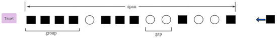
Figure 16.
Simplified parking lot (the black square represents the car, and the circle represents the parking space).
When entering the parking lot from the right side, the driver needs to walk to the far-left exit after finding a parking space. If the driver decides to park immediately upon entering the parking lot, they will have to walk a long distance after getting out of the car. On the other hand, if the driver continues driving forward upon entering the parking lot and actively seeks parking spaces near the exit, the walking distance after parking will be shorter. However, the unfortunate reality is that parking spaces near the exit are often in high demand, and drivers may end up empty-handed after spending time circling around in search of a spot. This wasted time and effort on circling back and forth can be frustrating.
Utilizing the principles of the A* algorithm, the parking lot is conceptualized as a graph. In this graphical representation, individual nodes correspond to available parking spaces. The edges between nodes signify viable pathways connecting adjacent parking spaces, with the weight of each edge representing the length of the respective path. This abstraction aims to facilitate the identification of the optimal parking space, employing the A* algorithm’s heuristic search capabilities. In response, three simple parking strategies can be obtained (as shown in Figure 17).
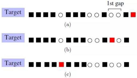
Figure 17.
Schematic diagram of the three strategies: (a) car discovery target; (b) car selection of parking space; (c) car final parking point.
Strategy A: After the car enters the parking lot, the first empty space found will be the target. As shown in Figure 17a, the car (red square) will be parked to the left of the first black square.
Strategy B: When the driver finds the first empty space, if there is still an empty space to the left of that space, the car will be parked to the left of that empty space; if there is no empty space to the left of that empty space, the car continues to drive forward to the end and then back up to the empty space closest to the exit. As shown in Figure 17b, the car is parked at the second vacant space at the entrance.
Strategy C: The driver keeps driving the car to the exit and then backs up to the empty space closest to the exit. If backing up to the entrance does not reveal an empty space, the process is repeated until the parking space closest to the exit is found. As shown in Figure 17c, the car is parked at the nearest empty space to the exit.
The drivers who adopt Strategy A do not waste time searching for parking spaces. Once they find an available spot, they park their vehicles. However, they often miss out on empty spaces near the exit. On the other hand, drivers who follow Strategy C take a gamble when they choose to constantly search for a vacant spot near the exit. In this continuous search, they waste time. Drivers who adopt Strategy B take a balanced approach. They pass the first available space, betting that there is at least one other empty spot in the parking lot.
Through modeling Strategy A, a certain connection between this strategy and micro dynamics was observed. For Strategy C and Strategy B, the study used differential formulas for modeling. To simplify the representation of the costs associated with these two strategies, the study graphically depicted the cost of time spent, as shown in Figure 18. When the parking lot situation is as shown in the upper part of Figure 18a, Strategy B does not require any backing up, whereas Strategy C requires some backing up, resulting in less time spent on Strategy B. When the parking lot situation is as shown in the lower part of Figure 18b, with no available parking spaces, both strategies require continuous backing up to find a spot, resulting in similar time costs.
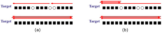
Figure 18.
Schematic diagram of the inter cost between Strategy B and Strategy C: (a) internal costs of Strategy B; (b)internal costs of Strategy C.
In summary, Strategy B incurs the least amount of time cost, followed closely by Strategy C, while Strategy A performs the worst. This is because Strategy A often results in parking far from the exit, leading to a long walking distance to reach the exit.
In turn, one can try to organize this study with mathematical calculations to simulate the coordinates of an ideal single-row parking lot (as shown in Figure 19).
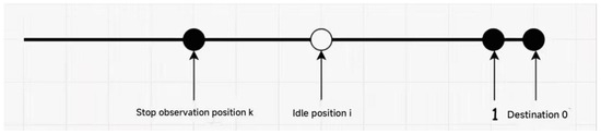
Figure 19.
Single-row parking.
Let x be the probability that a parking space is occupied; then, obviously, 1 − x is the vacancy rate, modeled after the 37% principle of one in a million.
Let k be the location where the driver starts to consider parking; then, the actual location i where parking is possible must satisfy at i < k. There are two more constraints:
- the driver parks at point i, which means there is no parking space in front of him, otherwise he may consider the space in front of him;
- If i is the optimal parking space, it means that there is no more parking space after i. Summing up the above two points, the probability of successful parking can be found as follows:
Derived:
Therefore,
The effect is optimal under this condition (as shown in Figure 20).
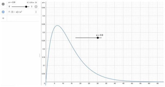
Figure 20.
Geogebra mapping.
This shows that, when the occupancy of a space is known to be a, the best choice is to start away from the destination and find a space and park in it. Given a, the corresponding k can be calculated.
3.2. Unmanned Vehicle Parking Modeling
The core idea of solving this problem is related to an iterative algorithm used to specify the set of unoccupied parking spaces. In the previous question, this paper has obtained the model of the parking process for different parking spaces and the model for determining the optimal parking space based on a random environment. Treating one vehicle entry and exit as a process, the random occupancy and release of parking spaces can be implemented using the random function. Each change of parking location in the process is accompanied by the calculation of the optimal parking model. After reiterating the algorithm 30 times, i.e., 30 processes, the simulation results of the driving trajectory from the current position in Figure 21 to the optimal parking space can be obtained.
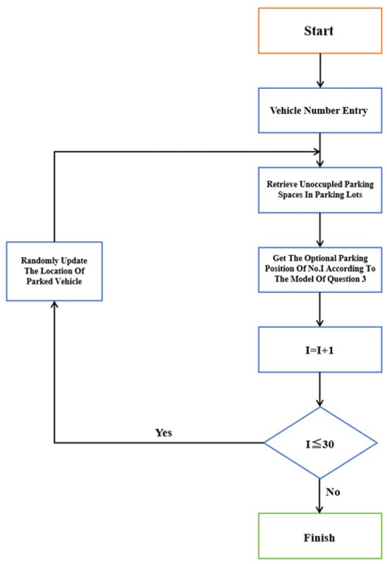
Figure 21.
Solution flow chart.
- In order to facilitate the study so that only one vehicle can enter at a time and adjacent vehicles will not have an impact on each other.
- The vehicles leave the parking space so that the neighboring vehicles enter the parking lot between t1(x1).t2(x2), respectively; then, Δt = t2(x2) − t1(x1).
- The number of vehicles leaving this parking lot in the Δt interval is randomly generated, and the corresponding parking space number is also randomly generated.
- In the process of vehicles entering the parking lot until the completion of the parking behavior, no other vehicles leave the parking space.
- The above algorithm was implemented and simulated using MATLAB 2021a.
3.3. Optimal Parking Space Driving Trajectory Simulation
Using MATLAB, the algorithm was implemented and simulated. Partial coding can be found in the Supplementary Materials (as shown in Figure 22).

Figure 22.
MATLAB parking simulation interface.
4. Conclusions
In conclusion, this paper designs a model of automatic parking path analysis using pre-target PID and a hybrid path-planning approach based on A* and the curve approach to optimize path tracking accuracy and demonstrate their effectiveness when applied to the Ackerman vehicle model, demonstrating their potential in solving challenges of driverless vehicles of various vehicle types.
The field of autonomous driving will reap huge benefits from the good functions of automatic parking. This momentum of technological progress will quickly move forward beyond traditional parking landscapes to include complex, dynamic, and unstructured environments.
A key avenue for further development is the convergence of real-time data and machine-learning techniques. By seamlessly adapting to a changing environment and drawing insights from previous experience, the automated parking system can iteratively improve its performance. Symsymbiotic relationship between autonomous parking systems and the transportation ecosystem. Through innovations such as vehicle-to-vehicle (V2V) and vehicle-to-infrastructure (V2I) communication technologies, these systems can leverage real-time insights to inform prudent parking decisions.
As the vision of technology expands, it becomes imperative to navigate its wider social and moral dimensions. Considering unpredictable human behavior and unforeseen circumstances is necessary. Furthermore, in the event of automatic parking system errors, the legal and insurance landscapes deserve careful inspection.
Ultimately, while the promise of automated parking technologies is bright and hopeful, they require a firm commitment to innovation, rigorous testing, and a comprehensive exploration of their impact. Its multiple strengths—including security, convenience, and efficiency—provide a fascinating canvas for continued research and development in the field, highlighting its significance in shaping a transformative future.
Supplementary Materials
The following supporting information can be downloaded at: https://www.mdpi.com/article/10.3390/wevj14120344/s1.
Author Contributions
Conceptualization, X.L. and Z.Z.; Methodology, S.Z.; Software, Y.F.; Validation, Y.F., Y.W. and Z.Z.; Formal Analysis, X.L. and Y.F.; Investigation, X.L.; Resources, X.L.; Data Curation, X.L.; Writing—Original Draft Preparation, X.L. and L.F.; Writing—Review and Editing, X.L. and W.L.; Visualization, X.L.; Supervision, X.L.; Project Administration, X.L. and Y.F. All authors have read and agreed to the published version of the manuscript.
Funding
This research was funded by the Fundamental Research Funds for the Central Universities (WUT: 2021IVB009).
Data Availability Statement
The authors attest that all data for this study are included in the paper.
Conflicts of Interest
The authors declare no conflict of interest.
References
- Sirithinaphong, T.; Chamnongthai, K. The recognition of car license plate for automatic parking system. In Proceedings of the ISSPA’99, the Fifth International Symposium on Signal Processing and Its Applications (IEEE Cat. No. 99EX359), Brisbane, Australia, 22–25 August 1999; IEEE: New York, NY, USA, 1999; Volume 1, pp. 455–457. [Google Scholar]
- Massaro, M.; Limebeer, D.J.N. Minimum-lap-time optimisation and simulation. Veh. Syst. Dyn. 2021, 59, 1069–1113. [Google Scholar] [CrossRef]
- Yu, Z.; Li, Y.; Xiong, L. Overview of Unmanned Vehicle Motion Planning Algorithms. J. Tongji Univ. (Nat. Sci.) 2017, 45, 1150–11591. [Google Scholar]
- Zhao, J.-S.; Liu, X.; Feng, Z.-J.; Dai, J.S. Design of an Ackermann-type steering mechanism. Proc. Inst. Mech. Eng. Part C J. Mech. Eng. Sci. 2013, 227, 2549–2562. [Google Scholar] [CrossRef]
- Marin, L.; Valles, M.; Soriano, A.; Valera, A.; Albertos, P. Event-based localization in ackermann steering limited resource mobile robots. IEEE/ASME Trans. Mechatron. 2013, 19, 1171–1182. [Google Scholar] [CrossRef]
- Behere, S.; Törngren, M. A functional architecture for autonomous driving. In Proceedings of the First International Workshop on Automotive Software Architecture, Montreal, QC, Canada, 4–8 May 2015; pp. 3–10. [Google Scholar]
- Wang, W.; Song, Y.; Zhang, J.; Deng, H. Automatic parking of vehicles: A review of literatures. Int. J. Automot. Technol. 2014, 15, 967–978. [Google Scholar] [CrossRef]
- Hsu, T.-H.; Liu, J.-F.; Yu, P.-N.; Lee, W.-S.; Hsu, J.-S. Development of an automatic parking system for vehicle. In Proceedings of the 2008 IEEE Vehicle Power and Propulsion Conference, Harbin, China, 3–5 September 2008; IEEE: New York, NY, USA, 2008; pp. 1–6. [Google Scholar]
- Bibi, N.; Majid, M.N.; Dawood, H.; Guo, P. Automatic parking space detection system. In Proceedings of the 2017 2nd International Conference on Multimedia and Image Processing (ICMIP), Wuhan, China, 17–19 March 2017; IEEE: New York, NY, USA, 2017; pp. 11–15. [Google Scholar]
- Faisal, A.; Kamruzzaman, M.; Yigitcanlar, T.; Currie, G. Understanding autonomous vehicles. J. Transp. Land Use 2019, 12, 45–72. [Google Scholar] [CrossRef]
- Schwarting, W.; Alonso-Mora, J.; Rus, D. Planning and decision-making for autonomous vehicles. Annu. Rev. Control Robot. Auton. Syst. 2018, 1, 187–210. [Google Scholar] [CrossRef]
- Kato, S.; Takeuchi, E.; Ishiguro, Y.; Ninomiya, Y.; Takeda, K.; Hamada, T. An open approach to autonomous vehicles. IEEE Micro 2015, 35, 60–68. [Google Scholar] [CrossRef]
- Fagnant, D.J.; Kockelman, K. Preparing a nation for autonomous vehicles: Opportunities, barriers and policy recommendations. Transp. Res. Part A Policy Pract. 2015, 77, 167–181. [Google Scholar] [CrossRef]
- Duarte, F.; Ratti, C. The impact of autonomous vehicles on cities: A review. J. Urban Technol. 2018, 25, 3–18. [Google Scholar] [CrossRef]
- Janai, J.; Güney, F.; Behl, A.; Geiger, A. Computer vision for autonomous vehicles: Problems, datasets and state of the art. Found. Trends® Comput. Graph. Vis. 2020, 12, 1–308. [Google Scholar] [CrossRef]
- Brenner, W.; Herrmann, A. An overview of technology, benefits and impact of automated and autonomous driving on the automotive industry. In Digital Marketplaces Unleashed; Springer: Berlin/Heidelberg, Germany, 2018; pp. 427–442. [Google Scholar]
- Yurtsever, E.; Lambert, J.; Carballo, A.; Takeda, K. A survey of autonomous driving: Common practices and emerging technologies. IEEE Access 2020, 8, 58443–58469. [Google Scholar] [CrossRef]
- Savkin, A.V.; Teimoori, H. Bearings-only guidance of a unicycle-like vehicle following a moving target with a smaller minimum turning radius. IEEE Trans. Autom. Control. 2010, 55, 2390–2395. [Google Scholar] [CrossRef]
- Domenici, P. The scaling of locomotor performance in predator–prey encounters: From fish to killer whales. Comp. Biochem. Physiol. Part A Mol. Integr. Physiol. 2001, 131, 169–182. [Google Scholar] [CrossRef] [PubMed]
- Howland, H.C. Optimal strategies for predator avoidance: The relative importance of speed and manoeuvrability. J. Theor. Biol. 1974, 47, 333–350. [Google Scholar] [CrossRef] [PubMed]
- Zhileykin, M.; Eranosyan, A. Algorithms for dynamic stabilization of rear-wheel drive two-axis vehicles with a plug-in rear axle. In IOP Conference Series: Materials Science and Engineering, Proceedings of the 245th ECS Meeting, San Francisco, CA, USA, 26–30 May 2024; IOP Publishing: Bristol, UK, 2020; Volume 963, p. 012010. [Google Scholar]
- Simionescu, P.A.; Beale, D. Synthesis and analysis of the five-link rear suspension system used in automobiles. Mech. Mach. Theory 2002, 37, 815–832. [Google Scholar] [CrossRef]
- Riedel-Lyngskær, N.; Petit, M.; Berrian, D.; Poulsen, P.B.; Libal, J.; Jakobsen, M.L. A spatial irradiance map measured on the rear side of a utility-scale horizontal single axis tracker with validation using open source tools. In Proceedings of the 2020 47th IEEE Photovoltaic Specialists Conference (PVSC), Calgary, AB, Canada, 15 June–21 August 2020; IEEE: New York, NY, USA, 2020; pp. 1026–1032. [Google Scholar]
- An, Z.; Meng, X.; Ji, X.; Xu, X.; Liu, Y. Design and performance of an off-axis free-form mirror for a rear mounted augmented-reality head-up display system. IEEE Photonics J. 2021, 13, 3052726. [Google Scholar] [CrossRef]
- Unser, M.; Aldroubi, A.; Eden, M. B-spline signal processing. I. Theory. IEEE Trans. Signal Process. 1993, 41, 821–833. [Google Scholar] [CrossRef]
- Gordon, W.J.; Riesenfeld, R.F. B-spline curves and surfaces. In Computer Aided Geometric Design; Academic Press: Cambridge, MA, USA, 1974; pp. 95–126. [Google Scholar]
- Buffa, A.; Sangalli, G.; Vázquez, R. Isogeometric methods for computational electromagnetics: B-spline and T-spline discretizations. J. Comput. Phys. 2014, 257, 1291–1320. [Google Scholar] [CrossRef]
- Parumasur, N.; Adetona, R.A.; Singh, P. Efficient solution of burgers’, modified burgers’ and KdV–burgers’ equations using B-spline approximation functions. Mathematics 2023, 11, 1847. [Google Scholar] [CrossRef]
- Briand, T.; Monasse, P. Theory and practice of image B-spline interpolation. Image Process. Line 2018, 8, 99–141. [Google Scholar] [CrossRef]
- Unser, M.; Aldroubi, A.; Eden, M. B-spline signal processing. II. Efficiency design and applications. IEEE Trans. Signal Process. 1993, 41, 834–848. [Google Scholar] [CrossRef]
- Wang, Y.; Tang, S.; Deng, M. Modeling nonlinear systems using the tensor network B-spline and the multi-innovation identification theory. Int. J. Robust Nonlinear Control. 2022, 32, 7304–7318. [Google Scholar] [CrossRef]
- Riedel, F. Optimal stopping with multiple priors. Econometrica 2009, 77, 857–908. [Google Scholar]
- Reikvam, K. Viscosity solutions of optimal stopping problems. Stoch. Stoch. Rep. 1998, 62, 285–301. [Google Scholar] [CrossRef]
- López, F.J.; San Miguel, M.; Sanz, G. Lagrangean methods and optimal stopping. Optimization 1995, 34, 317–327. [Google Scholar] [CrossRef]
- Svensson, L.; Masson, L.; Mohan, N.; Ward, E.; Brenden, A.P.; Feng, L.; Törngren, M. Safe stop trajectory planning for highly automated vehicles: An optimal control problem formulation. In Proceedings of the 2018 IEEE Intelligent Vehicles Symposium (IV), Changshu, China, 26–30 June 2018; IEEE: New York, NY, USA, 2018; pp. 517–522. [Google Scholar]
- Xu, J.; Chen, G.; Xie, M. Vision-guided automatic parking for smart car. In Proceedings of the IEEE Intelligent Vehicles Symposium 2000 (Cat. No. 00TH8511), Dearborn, MI, USA, 5 October 2000; IEEE: New York, NY, USA, 2000; pp. 725–730. [Google Scholar]
- Ma, S.; Jiang, H.; Han, M.; Xie, J.; Li, C. Research on automatic parking systems based on parking scene recognition. IEEE Access 2017, 5, 21901–21917. [Google Scholar] [CrossRef]
- Song, Y.; Liao, C. Analysis and review of state-of-the-art automatic parking assist system. In Proceedings of the 2016 IEEE International Conference on Vehicular Electronics and Safety (ICVES), Beijing, China, 10–12 July 2016; IEEE: New York, NY, USA, 2016; pp. 1–6. [Google Scholar]
- Jung, H.G.; Kim, D.S.; Yoon, P.J.; Kim, J. Parking slot markings recognition for automatic parking assist system. In Proceedings of the 2006 IEEE Intelligent Vehicles Symposium, Tokyo, Japan, 13–15 June 2006; IEEE: New York, NY, USA, 2006; pp. 106–113. [Google Scholar]
- Zhang, P.; Xiong, L.; Yu, Z.; Fang, P.; Yan, S.; Yao, J.; Zhou, Y. Reinforcement learning-based end-to-end parking for automatic parking system. Sensors 2019, 19, 3996. [Google Scholar] [CrossRef]
- Suhr, J.K.; Jung, H.G. Automatic parking space detection and tracking for underground and indoor environments. IEEE Trans. Ind. Electron. 2016, 63, 5687–5698. [Google Scholar] [CrossRef]
- Conejero, J.A.; Jordán, C.; Sanabria-Codesal, E. An iterative algorithm for the management of an electric car-rental service. J. Appl. Math. 2014, 2014, 483734. [Google Scholar] [CrossRef]
- Onieva, E.; Alonso, J.; Pérez, J.; Milanes, V.; de Pedro, T. Autonomous car fuzzy control modeled by iterative genetic algorithms. In Proceedings of the 2009 IEEE International Conference on Fuzzy Systems, Jeju, Republic of Korea, 20–24 August 2009; IEEE: New York, NY, USA, 2009; pp. 1615–1620. [Google Scholar]
- Divelbiss, A.W.; Wen, J.T. Trajectory tracking control of a car-trailer system. IEEE Trans. Control Syst. Technol. 1997, 5, 269–278. [Google Scholar] [CrossRef]
- Ritzinger, U.; Puchinger, J.; Hartl, R.F. A survey on dynamic and stochastic vehicle routing problems. Int. J. Prod. Res. 2016, 54, 215–231. [Google Scholar] [CrossRef]
- Jeong, S.; Jang, Y.J.; Kum, D. Economic analysis of the dynamic charging electric vehicle. IEEE Trans. Power Electron. 2015, 30, 6368–6377. [Google Scholar] [CrossRef]
- Yoerger, D.R.; Cooke, J.G.; Slotine JJ, E. The influence of thruster dynamics on underwater vehicle behavior and their incorporation into control system design. IEEE J. Ocean. Eng. 1990, 15, 167–178. [Google Scholar] [CrossRef]
- Kang, C.M.; Lee, S.H.; Chung, C.C. Comparative evaluation of dynamic and kinematic vehicle models. In Proceedings of the 53rd IEEE Conference on Decision and Control, Los Angeles, CA, USA, 15–17 December 2014; IEEE: New York, NY, USA, 2014; pp. 648–653. [Google Scholar]
- Rokonuzzaman, M.; Mohajer, N.; Nahavandi, S.; Mohamed, S. Model predictive control with learned vehicle dynamics for autonomous vehicle path tracking. IEEE Access 2021, 9, 128233–128249. [Google Scholar] [CrossRef]
- Chai, R.; Tsourdos, A.; Savvaris, A.; Chai, S.; Xia, Y.; Chen, C.L.P. Design and implementation of deep neural network-based control for automatic parking maneuver process. IEEE Trans. Neural Netw. Learn. Syst. 2020, 33, 1400–1413. [Google Scholar] [CrossRef] [PubMed]
- Zhao, J.; Zhang, X.; Shi, P.; Liu, Y. Automatic driving control method based on time delay dynamic prediction. In Proceedings of the Cognitive Systems and Signal Processing: Third International Conference, ICCSIP 2016, Beijing, China, 19–23 November 2016; Revised Selected Papers 3. Springer: Singapore, 2017; pp. 443–453. [Google Scholar]
- Li, X.; Li, Q.; Yin, C.; Zhang, J. Autonomous navigation technology for low-speed small unmanned vehicle: An overview. World Electr. Veh. J. 2022, 13, 165. [Google Scholar] [CrossRef]
- Backman, J.; Oksanen, T.; Visala, A. Navigation system for agricultural machines: Nonlinear model predictive path tracking. Comput. Electron. Agric. 2012, 82, 32–43. [Google Scholar] [CrossRef]
- Berclaz, J.; Fleuret, F.; Turetken, E.; Fua, P. Multiple object tracking using k-shortest paths optimization. IEEE Trans. Pattern Anal. Mach. Intell. 2011, 33, 1806–1819. [Google Scholar] [CrossRef]
- Jiang, H.; Fels, S.; Little, J.J. A linear programming approach for multiple object tracking. In Proceedings of the 2007 IEEE Conference on Computer Vision and Pattern Recognition, Minneapolis, MN, USA, 17–22 June 2007; IEEE: New York, NY, USA, 2007; pp. 1–8. [Google Scholar]
- Hua, L.; Chen, M.; Han, X.; Zhang, X.; Zheng, F.; Zhuang, W. Research on the vibration model and vibration performance of cold orbital forging machines. Proc. Inst. Mech. Eng. Part B J. Eng. Manuf. 2022, 236, 828–843. [Google Scholar] [CrossRef]
- Chen, M.; Zhang, X.; Zhuang, W.; Shu, Y.; Zhou, Z.; Xiong, W. Kinematics and dynamics simulations of cold orbital forging machines based on ADAMS. Proc. Inst. Mech. Eng. Part B J. Eng. Manuf. 2023, 237, 250–260. [Google Scholar] [CrossRef]
- Gu, Z.; Chen, M.; Wang, C.; Zhuang, W. Static and Dynamic Analysis of a 6300 KN Cold Orbital Forging Machine. Processes 2021, 9, 7. [Google Scholar] [CrossRef]
- Chen, M.; Ning, X.; Zhou, Z.; Shu, Y.; Tang, Y.; Cao, Y.; Shang, X.; Han, X. LMS/RLS/OCTAVE Vibration Controls of Cold Orbital Forging Machines for Improving Quality of Forged Vehicle Parts. World Electr. Veh. J. 2022, 13, 76. [Google Scholar] [CrossRef]
- Wang, Y.; Chen, L.; Zhou, L. Vehicle motion model and analysis of the “Tesla brake failure” event. Mech. Pract. 2022, 44, 852–856. [Google Scholar]
- Jiang, H.; Guo, K.; Zhang, J. Automatic parallel parking steering controller based on path planning. J. Jilin Univ. (Eng. Ed.) 2011, 41, 293–297. [Google Scholar] [CrossRef]
- Jiang, H. Research on Steering Control Strategy of Automatic Parallel Parking System. Ph.D. Thesis, Jilin University, Changchun, China, 2010. [Google Scholar]
- Wu, B. Research on Automatic Parking Path Simulation and Motion Control. Master’s Thesis, Hefei University of Technology, Hefei, China, 2012. [Google Scholar]
- Jiang, H.; Zhang, X.; Ma, S. Non time reference spiral curved ramp path tracking control for intelligent vehicles. J. Chongqing Univ. Technol. (Nat. Sci.) 2018, 32, 1–6. [Google Scholar]
- Guo, K.; Li, H.; Song, X.; Huang, J. Research on Path Tracking Control Strategy of Automatic Parking System. Chin. J. Highw. Eng. 2015, 28, 106–114. [Google Scholar] [CrossRef]
Disclaimer/Publisher’s Note: The statements, opinions and data contained in all publications are solely those of the individual author(s) and contributor(s) and not of MDPI and/or the editor(s). MDPI and/or the editor(s) disclaim responsibility for any injury to people or property resulting from any ideas, methods, instructions or products referred to in the content. |
© 2023 by the authors. Licensee MDPI, Basel, Switzerland. This article is an open access article distributed under the terms and conditions of the Creative Commons Attribution (CC BY) license (https://creativecommons.org/licenses/by/4.0/).