1. Introduction
Adaptive cruise is also known as adaptive cruise control. The adaptive cruise control system is an upgrade of the cruise control function. Compared with the cruise control function, the adaptive cruise control system reduces the actions that the driver needs to perform to cancel and set the cruise control function, and it is applicable to more road conditions. In short, adaptive cruise control can not only set the vehicle speed according to the driver’s requirements, but also automatically adjust the car by controlling the engine and brakes appropriately without the driver’s intervention. By installing a radar at the front of the car to continuously scan the road ahead of the vehicle and collecting the wheel speed measured by the wheel speed sensor, the car’s driving speed can be calculated. When the car is too close to the vehicle in front, the adaptive cruise control unit can also control the anti-lock braking system, engine control system, etc., to make the car wheels brake appropriately and reduce engine power, thereby maintaining a certain safe distance from the vehicle in front. The adaptive cruise control function mainly includes radar sensors, ultrasonic distance sensors, infrared distance sensors, digital signal processors, and control modules. When the adaptive cruise control function is in operation, the precise position of the vehicle in front is measured through the fusion of multiple sensors such as low-power radar or infrared beams. When the vehicle in front begins to slow down or new targets appear, the automatic driving system will send a signal to the brake to reduce speed, allowing the car and the vehicle in front to achieve safe-distance following. When there are no cars in front or the car in front changes lanes, the adaptive cruise control system will allow the car to drive safely according to the set speed, and the radar will continuously detect targets in the front and adjust the vehicle speed based on the actual road conditions. Adaptive cruise is widely recognized as a key component of the future autonomous vehicle [
1]. Therefore, the field has received widespread attention from scholars both domestically and internationally in recent years [
2]. Currently, the control design of the adaptive cruise control system mainly adopts double-layer control [
3]. The upper controller is based on the driving environment detected by the onboard sensors to calculate the corresponding expected acceleration, while the lower controller controls the brake and throttle based on the expected acceleration obtained by the upper controller to achieve the corresponding acceleration of the target vehicle. Fuzzy PID control, sliding mode control, model predictive control, and other traditional control methods have been widely used in ACC systems [
4,
5,
6]. These control methods take distance control as the main objective, obtaining the corresponding expected acceleration based on the safe distance to determine whether the vehicle needs to accelerate or decelerate. However, they do not take into account the perturbation changes in the vehicle’s own parameters and the inability of the vehicle to achieve the expected acceleration due to external interference. This article is based on the μ control theory, a two-stage adaptive cruise control method that considers robustness, safety, and comfort, is proposed to improve the system robustness performance and stability, as well as enhance the system anti-interference.
2. Adaptive Cruise Longitudinal Kinematics Model between Vehicles
In the process of natural driving, the driver will follow the vehicle in front at a certain speed and distance. With a change in the speed of the vehicle in front, the driver will use the accelerator pedal and brake pedal to adjust the safety distance between itself and the car in front and the speed of itself, so as to make the controlled car and the tracking vehicle maintain a certain distance and make the speed of the controlled vehicle consistent with the tracking vehicle, that is, the “two unchanged” principle [
7].
The two principles of invariance can be expressed through formulas as follows:
where the
represents the speed of the front vehicle,
represents the self-driving speed,
is the expected distance between cars, and
represents the actual distance between cars.
From the perspective of safe driving, the safe distance that two vehicles need to maintain when driving on a flat road mainly includes three aspects: firstly, the distance that the driver of the following vehicle can recognize and react during the time when the preceding vehicle slows down and brakes; the second is the delay caused by the acceleration process of two cars; and the third is the required distance between the front and rear cars after eliminating the relative speed between the two cars.
The longitudinal kinematics model between cars is shown in
Figure 1.
Figure 1.
Longitudinal kinematics model between cars.
Figure 1.
Longitudinal kinematics model between cars.
where
is the necessary safety distance, and the expected distance
between cars can be expressed as:
where
represents the vehicle speed before the preceding vehicle begins to decelerate,
represents the maximum acceleration of the self-driving vehicle,
represents the maximum acceleration of the preceding vehicle,
is the driver’s reaction time, and
is the safe distance that needs to be maintained when the two vehicles stop.
3. Upper Controller Design
The upper controller calculates the expected acceleration according to the speed and acceleration of the target controlled vehicle and the relative speed and distance from the vehicle in front.
According to the minimum safe distance model between cars, the kinematics relationship between the self-car and the front car can be expressed as:
where
is the difference between the actual distance of two vehicles and the expected safe distance, and
is the relative speed of the two vehicles.
With
and
as the state variables and the self-acceleration as the control variable, the equation of state of the longitudinal dynamics model between cars can be obtained as follows:
where
,
,
,
,
.
The control objective of the adaptive cruise upper controller is to make
and
simultaneously approach 0. Since safety is the most important and fundamental performance indicator of the ACC system, designing it as a soft constraint will increase safety hazards. Therefore, here we designed the safety indicator as a hard constraint.
The comfort of driving directly affects the level of acceptance of ACC by drivers and passengers. According to research, the smaller the change in acceleration, the higher the passenger’s sitting comfort and following adaptability. Therefore, while ensuring safety, the smaller the change in acceleration, the better [
8], i.e.,
.
Then, we take the minimum expected acceleration control index function for the car following as:
where
x is the state variable,
u is the control variable,
Q is the state weight matrix, and
R is the control weight matrix.
Q indicates the weighting of vehicle spacing and acceleration, and since this article comprehensively considers comfort and safety, the same weight value is taken. The selection of
R affects the control quantity. As the importance of control indicators on controlling energy consumption decreases, the tracking ability of the system under the corresponding controller control increases, and the control quantity, i.e., the amplitude of vehicle acceleration, also increases. If the order of magnitude difference between weight coefficients is too large, some sub objectives have too little impact on the optimization results and are easily overlooked, so it is necessary to limit the order of magnitude of each weight coefficient. Therefore, the value of
Q is
, and the value of
R is 0.05.
By using the Riccati method to solve the LQR upper controller in the LQR toolbox of MATLAB, the state feedback coefficient in the linear–quadratic regulator is:
4. Vehicle Longitudinal Dynamics Model
Before establishing the vehicle longitudinal dynamics model, the following assumptions should also be added:
- (1)
Simplify the four-wheel model into a two-wheel model, taking into account the uniformity of the vehicle’s overall weight and the load difference between the left and right wheels.
- (2)
Without considering the tire slip characteristics, the road can provide sufficient road adhesion coefficient when the car is driving, thereby maximizing the braking effect [
9].
The force acting on the vehicle during driving is shown in
Figure 2.
Among them,
represents the longitudinal driving speed,
represents the overall mass of the vehicle,
and
represent the braking torque of the front and rear wheels of the vehicle,
represents the air resistance during driving,
and
represent the friction force of the front and rear wheels from the road,
represents the driving torque provided by the engine, and
represents the wheelbase from the front to the rear wheels.
where
and
represent the load of the front and rear wheels, while
and
represent the distance from the front and rear axles of the car to the center of mass.
Equations of motion of the front and rear wheels as:
where
and
represent the moment of inertia of the front and rear wheels, respectively,
f represents the rolling resistance coefficient,
r represents the wheel radius, and
represents the wheel angular speed.
According to the longitudinal force condition of the vehicle during driving, the equations of motion can be established as follows:
In the equation:
Braking force: ;
Air resistance: ;
Rolling friction: .
Union can obtain:
where
is the braking coefficient,
is the total braking pressure,
is the air resistance coefficient,
A is the car windward area, and
is the density of air.
5. Lower-Level Controller Design Based on μ Control Method
Due to the complexity of the controlled objects in existing control systems and the wide range of application fields, the influence of uncertainty factors becomes more prominent in actual control system design. In order to achieve robust performance control of closed-loop control systems for controlled objects with multiple uncertain perturbation factors, Scholar Doyle proposed μ control theory in 1982, which explains that all discrete uncertainties can be concentrated in a diagonal matrix with known structural dimensions. The core idea of the μ control method is to analyze multiple unstructured perturbations/disturbances and other uncertain factors of the controlled object, transforming the performance robustness problem of the control system into a stability robustness problem; combining the robustness requirements of performance and stability, the control system is analyzed and synthesized. Meanwhile, the uncertainty factors are structured, which can provide a more reasonable analysis of the robustness and performance robustness of the control system, and to some extent, it reduces the conservatism problem of the H∞ control algorithm. The μ control theory involves reconstructing various aspects of the system, such as input, output, parameter perturbations, and transfer functions, in order to separate disturbances in advance.
In the presence of parameter changes in the vehicle, uncertainty in model modeling, and noise interference from external acceleration and speed, the lower layer μ controller is proposed to control the acceleration of the car and enable it to smoothly follow the expected acceleration outputted by the upper controller. According to the nominal model of the controlled system, the model uncertainty, the parameter perturbation of the model and the weight function satisfying the tracking effect, an augmented open-loop control system of the controlled object is established, and the D-K iterative algorithm is used to solve the controller according to the input–output relationship of the established open-loop system.
The design of the adaptive cruise lower controller needs to meet the following points:
- (1)
To ensure the tracking ability of the vehicle, the primary goal of the entire control system is to reduce the error between the actual acceleration of the vehicle and the expected acceleration outputted by the upper controller, so that the cruise system has a strong ability to follow cars.
- (2)
Considering the disturbance of vehicle parameters, model uncertainty, and other disturbance factors, as well as the stability of the vehicle during driving, higher requirements are put forward for the control of the system. In the real car-following process, the speed of the front car and the distance between the main car and the front car are measured by onboard radar sensors, while the main car uses wheel speed sensors and acceleration sensors to obtain information such as vehicle speed and acceleration. Due to the various state information of the system being affected by external disturbances, noise in the measured signal is inevitable. Therefore, the controller should have good anti-interference performance.
5.1. Inverse Longitudinal Dynamic Model
Since the engine and brake of the vehicle are both strong nonlinear elements, considering the problems of model simplification and calculation convenience, the inverse longitudinal dynamic model is established. In the inverse longitudinal dynamics model, the expected acceleration is input, and the engine torque and vehicle braking torque are obtained based on the longitudinal force balance analysis of the vehicle during driving. The establishment of the inverse longitudinal dynamics model greatly simplifies the establishment of the adaptive cruise system model, as shown in
Figure 3 [
10].
When the car is driving at a constant speed and in equilibrium, the driving force and resistance of the car in the longitudinal direction are calculated according to Newton’s law. The driving equation is:
In actual driving, when the car’s engine controls the speed, the brakes are in a state of non-operation. Ignoring the magnitude of the braking force,
, the output torque of the engine can be expressed as:
where
is the combined resistance force, and
is the expected engine driving force. Similarly, when the vehicle’s speed is controlled by the braking system, the acceleration obtained from the upper controller is input into the established reverse braking model,
, and the expected braking pressure can be obtained:
where
is the proportional coefficient, and
is the expected braking force.
Based on the characteristics of vehicle system response, it is proposed to use a first-order inert transfer function to connect the adaptive cruise vehicle inverse model and longitudinal dynamics model, namely:
5.2. Longitudinal Dynamic Perturbation Model
To construct the lower-level control model for the adaptive cruise control system, it is necessary to consider the uncertainties of the system. In the actual driving process, due to the difference in the unloaded and fully loaded states of the vehicle, the weight of the vehicle and the radius of the wheels will change within a certain range. The disturbance of these parameters will cause an increase in the acceleration overshoot of the control system, generate significant oscillations, and extend the adjustment time. Therefore, when designing a control system, it is necessary to take into account the perturbations of the system’s mass and radius in advance.
where
is the nominal vehicle mass,
is the nominal wheel radius,
is the change degree of the vehicle mass,
is the unit value perturbation of the vehicle mass,
represents the change degree of the wheel radius, and
represents the unit value perturbation of the wheel radius.
The perturbation model of the longitudinal dynamics of the vehicle can be expressed as:
In addition, the automobile’s engine and brake are strong nonlinear elements. In order to solve the problem concisely, the inverse model is used for linear connection. Thus, the model has the dynamic error of an unstructured model, which is expressed by the system multiplicative perturbation. Assuming
is the transfer function model of the system, the system model considering the multiplicative perturbation of the vehicle’s inverse longitudinal dynamics model is expressed as [
11]:
where
represents the normalized uncertainty function, and
represents the error weight function.
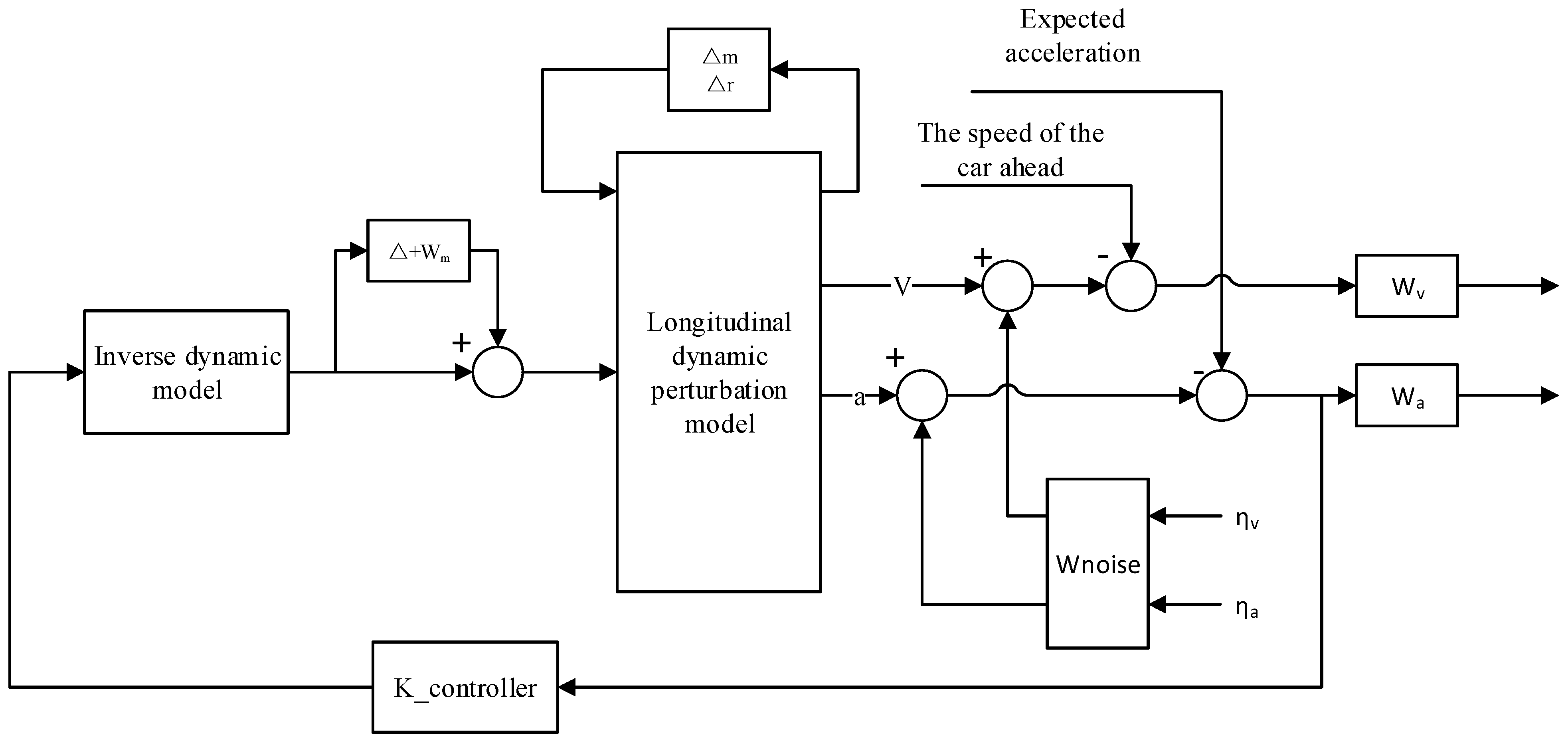
Add the sensor noise of the controller as an external interfere into the vehicle system model, and the lower layer μ control model can be obtained in
Figure 4 below.
In order to ensure the tracking ability of the vehicle and enable the cruise system to have a strong ability to following cars, one can reduce the value of , where is the expected acceleration output by the upper controller, is the actual output acceleration of the vehicle, and is the acceleration weight function. In order to ensure the safety performance of the vehicle and make the cruise system quickly reach the expected speed of the vehicle in front, one can reduce the value of , where is the speed of the vehicle in front, is the actual speed of the vehicle, and is the speed weight function.
When designing the lower brake controller of the system, the relevant signals of the vehicle are collected through speed and acceleration sensors and input into the system. Therefore, the noise disturbance to the control system mainly consists of two factors: the speed sensor noise and acceleration sensor noise, which are represented by and , and where and represent the weight function of velocity and acceleration. On this basis, this article tries to reduce the conservatism of the system model as much as possible, so that the designed weight function can be as close to the actual situation as possible. Meanwhile, considering the significant impact of the mid- to low-frequency range on the control system, it is important to avoid exceeding the perturbation gain when selecting the weight function. After multiple trials and calculations, taking specifically represents a velocity error of 0.13 m/s in the low-frequency range and 0.37 m/s in the high-frequency range. Taking specifically represents an acceleration error of 0.26 m/s2 in the low-frequency range and 0.3 m/s2 in the high-frequency range. For the uncertain model error of the system, one can select the weight function to indicate that the uncertain model error of the vehicle inverse model at low frequencies is 25%, while the uncertain model error at high frequencies is 100%.
5.3. Lower-Level Controller Design
The adaptive cruise lower controller adopts the μ control method to make the robust controller design, and the μ control method is an iterative algorithm based on a structural singular value [
12]. For the parameter uncertainty modules
,
, and the non-structural model dynamic error
, the mixed uncertainty diagonal matrix is defined as follows:
Establishing the system augmentation model
, which weights the output and interference, and obtaining the closed-loop control model of the uncertain system with weighting functions, are shown in
Figure 5 [
13,
14].
In
Figure 5,
M represents the lower linear fractional expression of the system model
and lower controller
K:
The transfer function relationship between the output
Z and input
W is:
For each controlled object on the uncertain set, if the controller can ensure its internal stability, it is called robust stability. If all objects in a set have internal stability and certain properties, it is called the “robustness” of the system. Robust control means that when the controlled object has uncertainty, it can ensure that the closed-loop system has good robust stability performance, that is, it is necessary to make each type of model of the controlled object in the disturbance area meet the required stability conditions and achieve the required performance indicators. The μ control theory solves the control
K through the D-K iterative algorithm, so that the controller
K satisfies [
15,
16]:
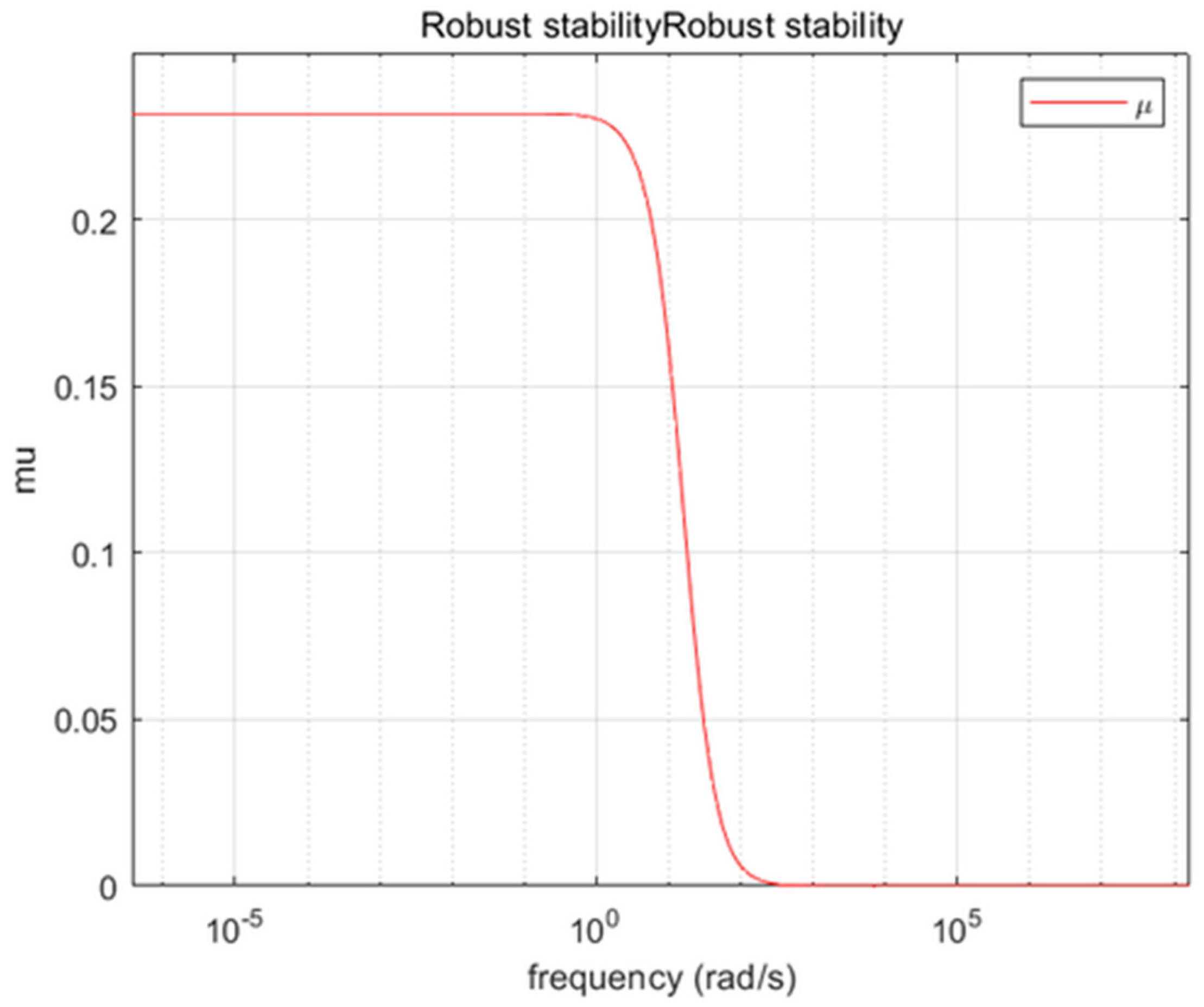
In MATLAB, based on the selected weight function, the robust control toolbox of MATLAB is used to solve the μ controller of the active collision avoidance open-loop braking control system. The frequency domain simulation results of the controller are shown in
Figure 6 and
Figure 7.
Figure 6 and
Figure 7 represent the performance structure singular values and perturbation structure singular values of the closed-loop system of the μ braking controller. It can be seen that the maximum value of the μ value of the designed active collision avoidance μ control system is 0.262 < 1. According to the μ control theory, it can be inferred that the designed μ braking controller has good performance robustness and robust stability under parameter uncertainty and various external disturbances, which can meet the performance requirements of the active collision avoidance braking system and demonstrate good anti-interference performance.
After five D-K iterations, the state space equation of the μ controller is:
The solution of the controller is obtained as:
6. Simulation Verification and Analysis
The overall parameters of the vehicle are show in
Table 1:
In order to verify the anti-interference performance of the designed controller, two working conditions were designed based on Simulink for simulation verification; at the same time, the H∞ and PID lower controllers were designed for comparison.
Condition 1: Set the initial speed of the own vehicle as 30 km/h, the initial speed of the front vehicle as 30 km/h, and the distance between the two vehicles as 30 m. The preceding vehicle decelerates at 3 s, accelerates at 4.5 s, and moves at a constant speed at 6 s. The simulation results are shown in
Figure 8,
Figure 9 and
Figure 10.
From
Figure 8 and
Figure 9, it can be seen that the acceleration and velocity tracking performance of the μ controller is better than that of the H∞ control and PID. The μ controller reached stability at 6.5 s, while the PID and H∞ control reached stability at 8.2 s.
Figure 10 shows the error between the actual distance of two vehicles and the expected safe distance under the three controllers. The error fluctuation range of the μ controller is around 0.05 m, while the error fluctuation of the H∞ control and PID control is relatively large, about 0.5 m.
Condition 2: Set the initial speed of the own vehicle as 30 km/h, the initial speed of the front vehicle as 30 km/h, and the distance between the two vehicles as 30 m. The front vehicle decelerates first at 3 s, accelerates at 4.5 s, and moves at a constant speed at 6 s. Controlling the mass of the vehicle to increase by 25% and verifying the control effect of the μ controller under model distortion, the simulation results are shown in
Figure 11,
Figure 12 and
Figure 13.
Figure 11 and
Figure 12 show that with a 25% increase in mass, the μ controller tends to stabilize at 6.36 s, while the H∞ control tends to stabilize at 8.3 s, and the PID control reaches stability at 8.54 s.
Figure 13 shows the error between the actual distance of two vehicles and the expected safe distance under the three controllers. The error fluctuation range of the μ controller is around 0.05 m, while the fluctuation range of the PID control is increased to 0.6 m, which is greatly affected by model distortion. The simulation results indicate that the designed μ controller significantly improves the anti-interference performance of the system.
7. Conclusions
The thesis focuses on the issue of driving comfort during the following cruise process, as well as the speed, accuracy, and safety of the vehicle response. Based on the optimal control method, the LQR upper controller was designed. By establishing the longitudinal dynamics model between vehicles, the optimal control acceleration was calculated, which improved the comfort and reliability of autonomous following while ensuring safety. Considering the uncertainty of its own model and the impact of parameter perturbations on control effectiveness, a longitudinal dynamic perturbation model was established to make the model more in line with the situation of vehicle following, which improved the accuracy and reliability of the model. And, based on the μ control method, we designed the lower controller, which improved the robustness of the autonomous following system. Through simulation verification and comparison with the H∞ controller and PID controller, it can be seen that the designed dual-layer controller has better anti-interference performance and corresponding performance, and can accurately follow the vehicle in front. Therefore, the cruise controller designed here can ensure good tracking, safety, and comfort of the vehicle, laying the foundation for further research on active safety technology.
However, when modeling the vehicle dynamics system in this thesis, only the longitudinal dynamics control problem was considered, and the vehicle model was simplified with a two-wheel model. In future research, further consideration can be given to constructing a four-wheel model of the entire vehicle, while integrating lateral and longitudinal motion control of the vehicle. Meanwhile, in terms of the design of the robustness μ controller, this article only studied and analyzed the effects of mass, wheel radius perturbation, and unmodeled errors on the braking control system regarding the self-vehicle parameter perturbations that exist during actual driving. In future research, other uncertain factors with practical effects, such as the road adhesion coefficient, system response time, etc., can be added to consider their impact on adaptive cruise control.
Author Contributions
Conceptualisation, Z.Z., B.L. and S.B.; methodology, S.B. and Z.Z.; software, Z.Z.; validation, G.L., S.B. and B.L.; formal analysis, Z.Z.; investigation, S.B. and G.L.; resources, B.L., C.G. and H.T.; data curation, Z.Z. and C.G.; writing—original draft preparation, Z.Z.; writing—review and editing, Z.Z.; visualisation, Y.Z.; supervision, B.L.; project administration, B.L.; funding acquisition, S.B. All authors have read and agreed to the published version of the manuscript.
Funding
This research was funded by the National Natural Science Foundation of China under grant number 52172367, The Natural Science Foundation of the Jiangsu Higher Education of China under grant number 21KJA580001, and Changzhou International Science and Technology Cooperation Fund under grant number CZ20220031. The APC was funded by 52172367.
Data Availability Statement
Not applicable.
Conflicts of Interest
The authors declare no conflict of interest.
References
- Vahidi, A.; Eskandarian, A. Research advances in intelligent collision avoidance and adaptive cruise control. IEEE Trans. Intell. Transp. Syst. 2004, 4, 143–153. [Google Scholar] [CrossRef]
- Yang, L.; Zhao, X.; Wu, G.; Xu, Z.; Barth, M.; Hui, F.; Hao, P.; Han, M.; Zhao, Z.; Fang, S.; et al. Overview of Collaborative Ecological Driving Strategies for Intelligent Connected Vehicles. J. Traffic Transp. Eng. 2020, 20, 58–72. [Google Scholar]
- Zhang, J.; Ioannou, P.A. Longitudinal control of heavy trucks in mixed traffic: Environmental and fuel economy considerations. IEEE Trans. Intell. Transp. Syst. 2006, 7, 92–104. [Google Scholar] [CrossRef]
- Hu, Z.; Su, R.; Zhang, K.; Xu, Z.; Ma, R. Resilient Event-Triggered Model Predictive Control for Adaptive Cruise Control Under Sensor Attacks. IEEE/CAA J. Autom. Sin. 2023, 10, 807–809. [Google Scholar] [CrossRef]
- Wu, G.; Guo, X.; Zhang, L. Design of Multi objective Robust control Control Algorithm for Vehicle Adaptive Cruise Following. J. Harbin Inst. Technol. 2016, 48, 80–86. [Google Scholar]
- Gao, C.Z. Target Vehicle Selection Algorithm for Adaptive Cruise Control Based on Lane-changing Intention of Preceding Vehicle. J. Mech. Eng. 2021, 34, 390–407. [Google Scholar]
- Liu, Q.; Yang, L.; Gao, B.; Wang, J.; Li, K. Intelligent car following model based on cognitive risk Dynamic equilibrium. Automot. Eng. 2022, 44, 1627–1635. [Google Scholar]
- Jenness, J.W.; Lerner, N.D.; Mazor, S.; Osberg, J.S.; Tefft, B.C. Use of Advanced In-Vehicle Technology by Young and Older Early Adopters; NHTSA: Washington, DC, USA, 2008; pp. 810–828.
- Pan, Y.; Nie, X.; Li, Z.; Gu, S. Data-driven vehicle modeling of longitudinal dynamics based on a multibody model and deep neural networks. Measurement 2021, 180, 109541. [Google Scholar] [CrossRef]
- Lien, C.; Shen, C.; Chang, H.; Hou, Y.; Yu, K. Mixed performance for robust fuzzy control of nonlinear autonomous surface vehicle via T-S model approach. Asian J. Control 2022, 24, 1059–1073. [Google Scholar] [CrossRef]
- Liu, Y. Research on Longitudinal Dynamic Model and Control Strategy for Active Collision Avoidance. J. Jiangsu Univ. 2016, 174–193. [Google Scholar]
- Xie, Y.; Wei, Z.; Zhao, L.; Jia, W.; Wu, C. Base on μ Robust lateral control for human-machine co driving of intelligent vehicles using a comprehensive approach. J. Mech. Eng. 2020, 56, 104–114. [Google Scholar]
- Wang, Y.; Gao, S.; Wang, Y.; Wang, P.; Zhou, Y.; Xu, Y. Robust trajectory tracking control for autonomous vehicle subject to velocity-varying and uncertain lateral disturbance. Arch. Transp. 2021, 57, 7–23. [Google Scholar] [CrossRef]
- Green, M. H∞ controller synthesis by J-lossless coprime factorization. SIAM J. Control Optim. 1992, 30, 522–547. [Google Scholar] [CrossRef]
- Zhou, B.; Wu, X.; Wei, G. Base on μ Research on Robust control Control of Integrated Vehicle Active suspension. J. Vib. Eng. 2017, 30, 1029–1037. [Google Scholar]
- Guo, N.; Zhang, X.; Zou, Y. Real time predictive control of path following to stabilize autonomous electric vehicles under extreme drive conditions. Automot. Innov. 2022, 5, 453–470. [Google Scholar] [CrossRef]
| Disclaimer/Publisher’s Note: The statements, opinions and data contained in all publications are solely those of the individual author(s) and contributor(s) and not of MDPI and/or the editor(s). MDPI and/or the editor(s) disclaim responsibility for any injury to people or property resulting from any ideas, methods, instructions or products referred to in the content. |
© 2023 by the authors. Licensee MDPI, Basel, Switzerland. This article is an open access article distributed under the terms and conditions of the Creative Commons Attribution (CC BY) license (https://creativecommons.org/licenses/by/4.0/).


 ,
, 


