Vehicle Lateral Velocity Estimation Based on Long Short-Term Memory Network

Abstract

Lateral velocity is an important parameter to characterize vehicle stability. The acquisition of lateral velocity is of great significance to vehicle stability control and the trajectory following control of autonomous vehicles. Aiming to resolve the problems of poor estimation accuracy caused by the insufficient modeling of traditional model-based methods and significant decline in performance in the case of a change in road friction coefficient, a deep learning method for lateral velocity estimation using an LSTM, long-term and short-term memory network, is designed. LSTM can well reflect the inertial characteristics of vehicles. The training data set contains sensor data under various working conditions and roads. The simulation results show that the prediction model has high accuracy in general and robustness to the change of road friction coefficient.

1. Introduction

With the continuous growth of car ownership, the frequency of traffic accidents has increased year by year [1]. To improve vehicle safety and reduce the frequency of accidents, a large number of active control systems (ACSs) are assembled in vehicles during mass production. These systems mainly include active front wheel steering (AFS), electronic stability program (ESP), and traction control systems (TCS). In addition, with the continuous improvement of vehicle intelligence, advanced driver assistance systems (ADAS) are also widely used [2], including adaptive cruise control (ACC) and lane keeping assistance (LKA) systems.

The advanced active control systems and advanced driver assistance systems are achieved based on the acquisition of some basic states of the vehicle [1,3], such as vehicle sideslip angle, yaw rate, longitudinal speed, and lateral speed, etc. However, due to limited sensor accuracy and cost as well as the difficulty in determining the distribution characteristics of measurement noise, some states or parameters cannot be effectively measured using applicable sensors, or measurement performance cannot meet the accuracy requirements.

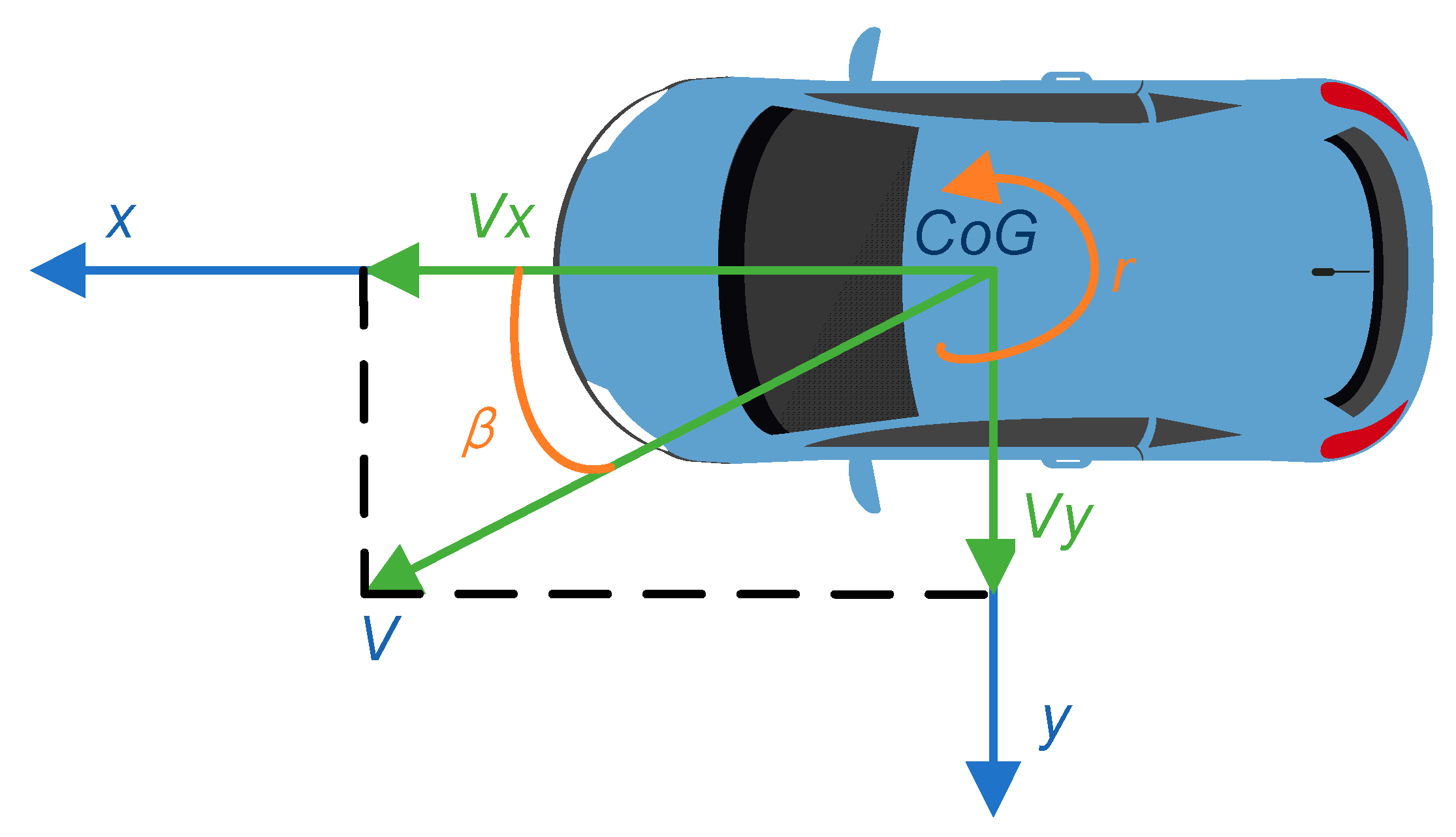
Among these states, the sideslip angle of the vehicle is closely related to the kinematic and dynamic response, which is expressed as an arctangent function of the ratio of vehicle lateral speed to longitudinal vehicle speed (show in Figure 1). Under linear working conditions, longitudinal speed can be obtained by fusing the speed sensors placed on the wheel. However, due to the lack of direct sensors, the lateral velocity cannot be obtained directly.

Therefore, it has become a research hotspot in automotive engineering field to estimate the lateral velocity or sideslip angle using existing low-cost sensors combined with estimation algorithms. These works can be divided into two categories, namely model-based and neural network (NN)-based methods [4,5], where the former uses kinematic and dynamic models to describe the relationship between sideslip angle and other vehicle parameters. The performance of a model-based estimator depends on vehicle modeling and sensor accuracy. However, the nonlinear characteristics and changing working conditions of the vehicle model make it difficult to obtain satisfactory estimation performance.

The neural network model can be used to describe vehicle dynamics [6,7] without understanding the inherent parameters of the vehicle. With an appropriate model structure as well as rich and diverse training data, the neural network-based method can accurately and effectively estimate the dynamic state of the vehicle, as shown in some preliminary studies [8]. In addition to direct lateral velocity estimation, the estimation results can also be used as the input of the model-based comprehensive estimator [9], which is known as a pseudo multi-sensor fusion.

However, at present, the training data and verification data of neural network-based methods are not universal because they tend to be obtained under the same road conditions. In addition, the commonly used DNN model cannot reflect the relationship between the current state and past state of the vehicle, and thus cannot express the inertia characteristics of the vehicle.

In this paper, an estimation model of lateral velocity is constructed based on an LSTM, long-term and short-term memory network. Compared with a DNN network, LSTM can represent the dependence between current state and past state, which is more suitable for inertial system modeling. The model takes the timing signal of an on-board cheap sensor as the input. The network is simple in structure and can run in real time in a real vehicle environment. The verification results show that this method is superior to the traditional method under linear conditions and demonstrates certain robustness to the change of road friction coefficient.

The contributions of this paper are as follows:

• Proposing a method of estimating vehicle lateral velocity based on LSTM using the most common sensor measurements in mass production vehicles.
• Testing on roads with different road friction coefficients. The results show that the proposed method is robust to the change of road friction coefficient.
• Collecting a data set from multiple measurement data under generally standard working conditions rather than verification working conditions. The verification results show that training set can well reflect vehicle characteristics.

The rest of this paper is arranged as follows. Section 2 briefly introduces the common methods of lateral velocity estimation. Section 3 describes the lateral velocity estimation method proposed in this paper in detail. The verification results of the model are presented in Section 4. Finally, the results are discussed and summarized in Section 5.

2. Related Work

On the premise that the vehicle longitudinal speed is known, lateral speed is estimated to be equivalent to sideslip angle, and their relationship can be expressed as:

$$\beta =arctan\left(\frac{v_y}{v_x}\right)$$

(1)

The methods of lateral velocity estimation or sideslip angle estimation can be divided into model-based and neural network-based methods.

2.1. Model Based Approach

Model-based methods can be divided into three categories: Luenberger observer (LO), sliding mode observer (SMO), Kalman filter (KF) and its variants. They are applicable to both linear and nonlinear systems. Lo and SMO are deterministic observers, and they are simple, which is their main advantage. However, they assume a complete understanding of the system and its inputs, regardless of possible modeling errors or measurement noise. The KF-based method can use an approximate model and deal with measurement noise [10]. In addition, with robustness and stability, it is relatively simple to implement. Therefore, the method based on KF and its variants has become a mainstream.

Li et al. [11] proposed a fusion estimation method composed of a kinematics estimator and a motion geometry estimator. The kinematics estimator uses an extended Kalman filter (EKF) based on a 3-DOF (degree of freedom) single-track vehicle model as an observer. The results of the two estimators are fused based on the dynamic characteristic strength of sideslip angle to accurately estimate sideslip angle under dynamic and steady-state conditions. The estimation algorithm proposed by Zhou et al. [12] is based on the 7-DOF non-linear dynamic model, and combines the UKF algorithm with the genetic algorithm to achieve the adaptive effect of noise, greatly improving the estimation accuracy but with certain anti-interference ability.

2.2. Neural Network Based Approach

Recently, various neural network models have been proposed in the literature for estimating lateral velocity or sideslip angle. Liu et al. [13] compared the model-based method and neural network-based method in their research, and found that the performance of the latter is superior to that of the former in all aspects when the data set is appropriately selected.

Du et al. [14] used a back propagation neural network to predict sideslip angle. The results show that the estimation algorithm based on the neural network demonstrates good performance under high-speed conditions. Chindamo et al. [15] proposed a concise method to obtain training data under specific working conditions. Torben et al. [16] proposed a scheme based on the recurrent neural network. The results show that the method demonstrates good generalization performance under different tire, road, and driving conditions.

Sasaki et al. [17] proposed a simple feedforward neural network (FFNN) using only yaw rate and lateral acceleration as inputs. It represents the dependency between the cur-rent state and the past state and is approximated by adding a delay signal to the network input. The verification results show that the estimation performance is satisfactory in the linear region, while the estimation error will increase in the nonlinear or more dynamic region.

Abdulrahim et al. [18] installed four additional accelerometers in each corner of the car, and took the longitudinal and lateral acceleration output by them as the input of the FFNN network. When the actual sideslip angle reaches 70°, the error is as high as 10° (about 14%). However, its training data are limited to fixed tracks and do not include additional road conditions, so it is impossible to evaluate the generalization performance of the algorithm.

Melzi et al. [19] used steering wheel angle, chassis longitudinal and lateral acceleration, yaw rate, and wheel speed as inputs of the neural network. The delay in the way of TDNN is used to approximate the basic dynamics. The dataset used contains different pavements, so it has a certain generalization ability. The model shows that the effect is good in the range of small steering wheel input. The performance is poor when the side deflection angle is greater than 7°.

3. Method

In this section, the LSTM neural network is introduced first. Then, the problem of vehicle lateral velocity estimation is defined. Thirdly, the lateral velocity estimation model based on LSTM proposed in this article is presented, and finally the training process of the model.

3.1. Preliminary: LSTM Neural Network

The LSTM network and recurrent neural network (RNN) have similar chain structures, notwithstanding that each repeated unit of the former contains more complex components [20].

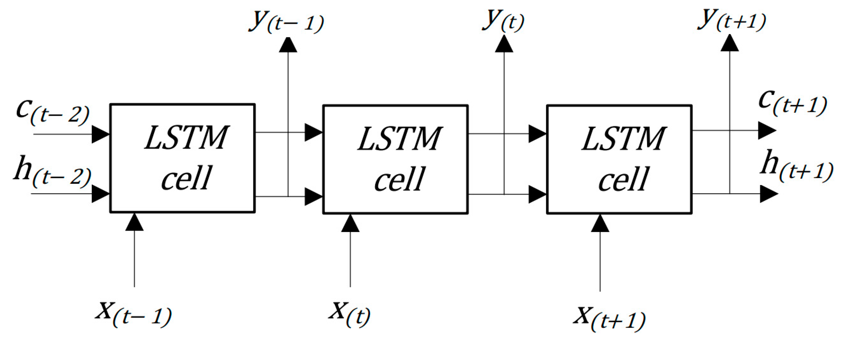
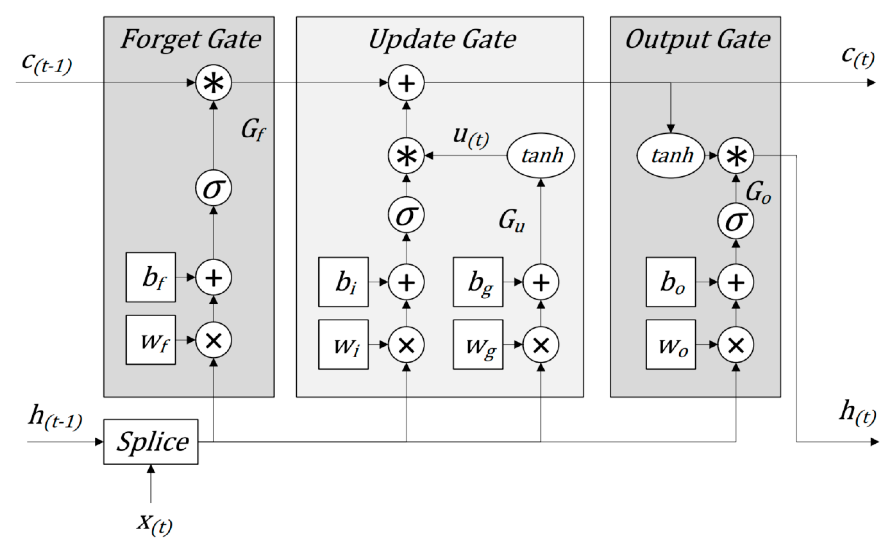
The sequential structure of LSTM network is shown in Figure 2, where the input of each repeating unit at time t includes sample input data $x_{\left(t\right)}$, the state of the previous unit $c_{\left(t-1\right)}$, and the output of the previous unit $h_{\left(t-1\right)}$. The detailed structure of the LSTM unit is shown in Figure 3.

In Figure 3, $w_f$ is the weight of the forgetting gate; $w_i$,$w_g$ is the weight of the update door; $w_o$ is the weight of the output gate; $b_f$ is the bias of the forget gate; $b_i$,$b_g$ is the bias of the update gate; $b_o$ is the bias of the output gate. Splicing means merging two vectors into one; $\sigma (⬝)$ indicates sigmoid activation function; $tanh(⬝)$ indicates hyperbolic tangent activation function; “ *” indicates multiplication by elements, and “+” indicates addition by elements.

The forget gate $G_f$ filters the non-discarded states of the previous unit through the sigmoid activation function:

$$G_f=\sigma \left(W_f^T\left[h_{\left(t-1\right)},x_{\left(t\right)}\right]+b_f\right)$$

(2)

The update gate $G_u$ determines the part to be updated, and $u_{\left(t\right)}$ provides alternative update data:

$$u_{\left(t\right)}=tanh\left(W_g^T\left[h_{\left(t-1\right)},x_{\left(t\right)}\right]+b_g\right)$$

(3)

$$G_u=\sigma \left(W_i^T\left[h_{\left(t-1\right)},x_{\left(t\right)}\right]+b_i\right)$$

(4)

The updated unit state $c_{\left(t\right)}$ consists of the selected state at the previous time and the newly selected alternative variable:

$$c_{\left(t\right)}=G_f\ast c_{\left(t-1\right)}+G_u\ast u_{\left(t\right)}$$

(5)

In the output link, $tanh\left(c_{\left(t\right)}\right)$ limits the value of $c_{\left(t\right)}$ to the range of (−1, 1). The output gate $G_o$ determines the part to be output to finally obtain the output of the unit $h_{\left(t\right)}$:

$$G_o=\sigma \left(W_o^T\left[h_{\left(t-1\right)},x_{\left(t\right)}\right]+b_o\right)$$

(6)

$$h_{\left(t\right)}=G_o\ast tanh\left(c_{\left(t\right)}\right)$$

(7)

3.2. Definition of Lateral Velocity Estimation Problem

As shown in Figure 1, the coordinate of the vehicle body is defined with a body-fixed coordinate system with the origin located at the center of gravity (CoG). The x-axis points in the forward direction of the vehicle, while the y-axis points to the left when the car is moving forward. The lateral velocity is the component of the vehicle’s speed at CoG along the y-axis.

Lateral velocity estimation is used to design a method to estimate the lateral velocity with cheap on-board sensors’ signals as the input, which can be expressed as:

$$V_y{}_{\left(t\right)}=f\left(Senso{r}_{input}^t, Senso{r}_{input}^{t-1}, Senso{r}_{input}^{t-2}, \dots \dots \right)$$

(8)

$Senso{r}_{input}^t$ represents the vector composed of all sensor measurements at time t. The estimation method is designed to find a function f. The output of the function is the lateral velocity at the current time, and its input can be the signals of the sensor at the current and previous time.

3.3. Lateral Velocity Estimation Model

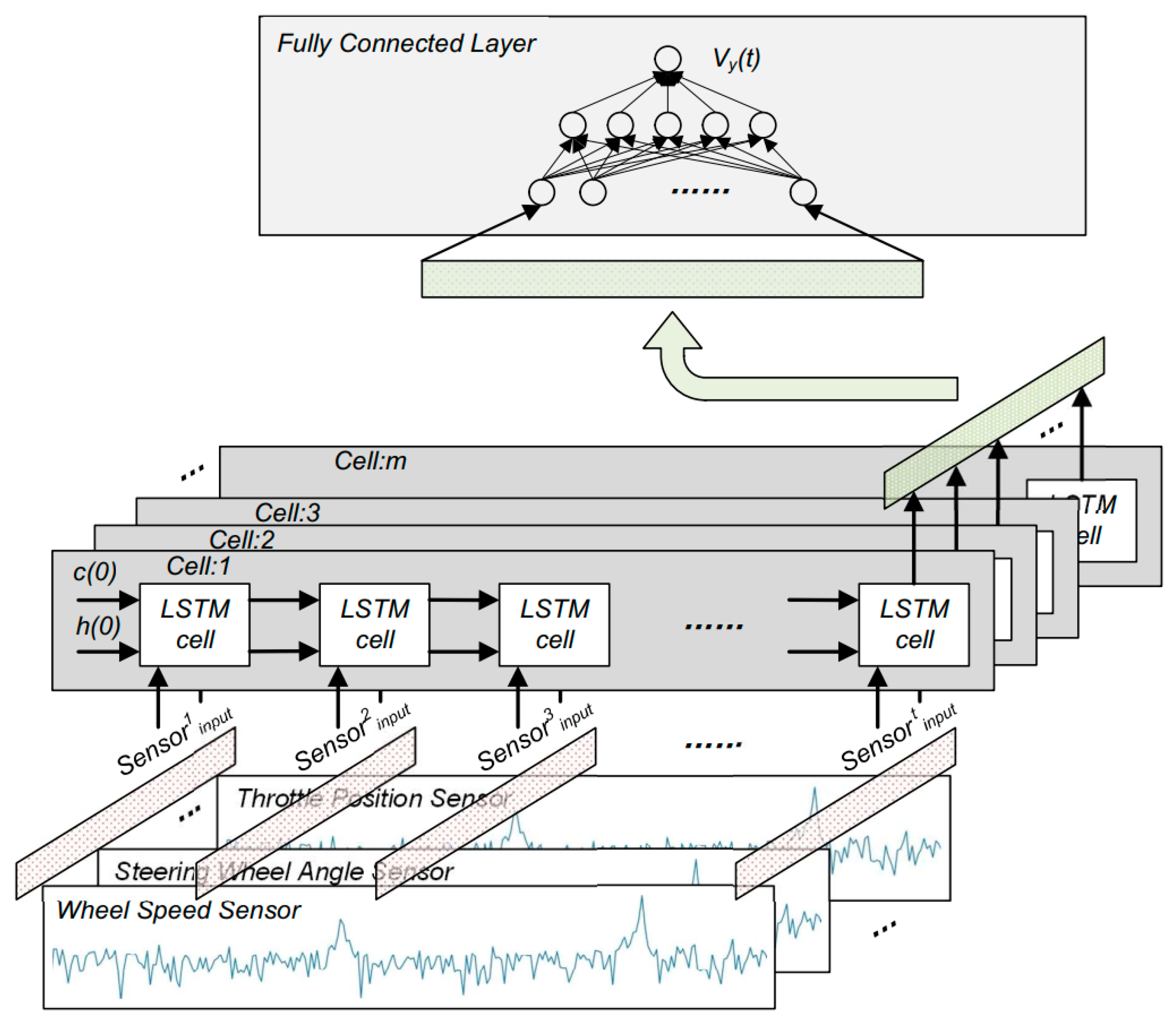
The architecture of the lateral velocity estimation method proposed in this paper is shown in Figure 4. It is divided into three layers: sensor input layer, LSTM layer, and fully connected layer. The sensor input layer is used to transform the original sensor signal into the input signal sequence required by the model. The LSTM layer is the main layer used to express the relationship between sensor input and lateral velocity. Due to the large number of units in the LSTM layer, the fully connected layer is used to limit the output dimension to 1.

The output is the lateral speed at the current time, and the input is the sensor signal of t steps which can be expressed as:$\left[Senso{r}_{input}^1, Senso{r}_{input}^2, \dots \dots ,Senso{r}_{input}^t\right]$. It is abbreviated as $Mode{l}_{input}$.

3.3.1. Sensor Input Layer

It is difficult to accurately express the relationship between lateral speed and other vehicle state parameters. The vehicle’s longitudinal speed, longitudinal acceleration, lateral acceleration, yaw rate, steering angle, and wheel speed may affect its lateral speed. In these dynamic states, the wheel speed can be obtained from the wheel speed sensor, the yaw rate and lateral acceleration of the vehicle can be obtained from the sensor of the ESP system or measured by IMU, the longitudinal speed can be obtained from the estimation result of the ESP system, the steering angle can be measured by the steering angle encoder, and the parameters related to the engine can be obtained from the engine control unit.

The traditional method based on the Kalman filter takes the steering wheel angle, yaw rate, and lateral acceleration signals as inputs.

Table 1. Sensor Input.

Sensor	Symbol	Unit
Steering wheel angle	$\delta$	deg
Throttle opening	$\alpha$	%
Engine speed	$n_e$	rpm
Gear	$G$	-
Left front wheel speed	${\omega }_{fl}$	rpm
Right front wheel speed	${\omega }_{fr}$	rpm
Left rear wheel speed	${\omega }_{rl}$	rpm
Right rear wheel speed	${\omega }_{rr}$	rpm
Longitudinal acceleration	$a_x$	g
Lateral acceleration	$a_y$	g
Yaw rate	$r$	deg/s
Longitudinal speed	$V_x$	km/h

summarizes the sensor inputs used in proposed estimation method. One step of the input can be expressed as a vector: ${\left[\delta ,\alpha ,n_e,G,{\omega }_{fl},{\omega }_{fr},{\omega }_{rl},{\omega }_{rr},a_x,a_y,r,V_x\right]}^T$. It is abbreviated as $Senso{r}_{input}^t$.

In the real vehicle, the sampling frequency of the sensors is different and needs to be unified to the same sampling frequency through down sampling or resampling. In this paper, the frequencies of 12 kinds of sensor signal are unified to 200 Hz, and the number of input steps to the LSTM layer is determined by hyperparameter tuning.

3.3.2. LSTM Layer

The LSTM layer can express the relationship between the state and the input at the current time and that between the state and input at the previous time, which is consistent with the characteristics of the vehicle as an inertial system, i.e., the lateral speed at the current time is related to the current input and the previous lateral speed, and its value is unlikely to change suddenly.

The LSTM layer may contain one or more hidden layers, each of which may contain multiple LSTM units. The LSTM unit obtains an output after processing one step of the input sequence. The outputs of multiple LSTM units in each hidden layer form a vector sequence, and the dimension of the vector is equal to the number of LSTM units. The out-put of each layer is a vector sequence, and that of the last layer is the last step of the vector sequence.

The numbers of units and hidden layers of the LSTM layer are also determined by hyperparameter tuning. Too many hidden layers will lead to the loss of information and reduce the training speed. Therefore, to improve the fitting ability of the model, the number of units is suggested to be increased.

3.3.3. Fully Connected Layer

The input of the fully connected layer is the last step of the vector sequence output by the last hidden layer of the LSTM. Since the output of the overall architecture is one-dimensional, and the last hidden layer in the LSTM layer may contain multiple units, a fully connected layer is added after the LSTM layer to limit the output dimension to one dimension. In addition, the fully connected layer can linearly combine the output characteristics of the LSTM layer.

The fully connected layer may contain multiple hidden layers, and each layer may have multiple units. The input of each unit is the output value of the units on the upper layer, and the unit will linearly combine these input values to obtain the output value through the activation function. The last layer contains only one unit, whose output value is the estimated value of lateral velocity.

3.4. Model Training

This section introduces the training process of the model proposed in this article. First, how to obtain the training data set and the composition of the data set are introduced. Then, the results of hyperparameter tuning and the training process of the model after tuning are introduced.

3.4.1. Data Set

It is dangerous and uneconomical to experiment on a real vehicle. In this study, we used the dynamic simulation software CarSim for experiments. CarSim has been widely accepted as a substitute for real vehicle experiments. For more information about Carism software, please refer to [21,22]

In this study, a light full-size car was selected as the experimental environment. The experimental data were obtained by fixed driver operation, vehicle speed, and road friction coefficient. Among them, the driver operated the J-turn on the left and right, the steering wheel angle was fixed at 40°, 60°, 90°, 100°, and 120°, the vehicle speed was set at 20–120 km/h, the interval was 10 km/h, and the road friction coefficient was set at 0.3, 0.5, 0.85, and 1.0.

The total length of the data set was 1 h 28 m 16 s, which was divided into 1,548,633 samples according to the length of the input sequence.

3.4.2. Hyperparameters Tuning

For the test sample, 10% of the data set was randomly selected, and 10% of the training samples were randomly selected as the verification set for the hyperparameter tuning. The final parameter setting is shown in

Table 2. Network Model Hyperparameters Setting.

Category	Parameter	Value
LSTM Layer	Hidden Layers	1
	Hidden Units	128
Full connection layer	Hidden Layers	1
	Hidden Units	64
	Output Layer Units	1
Overall Architecture	Input Sequence length	5
	Number of Parameters	80,513
	Activation Function	Relu
Training Process	Batch Size	32
	Initial Value of Learning Rate	0.001
	Early Stop Patience Value	5
Training Algorithm	Gradient Attenuation Factor	0.9
	Square Gradient Attenuation Factor	0.99
	Bias Term	1 × 10−8

.

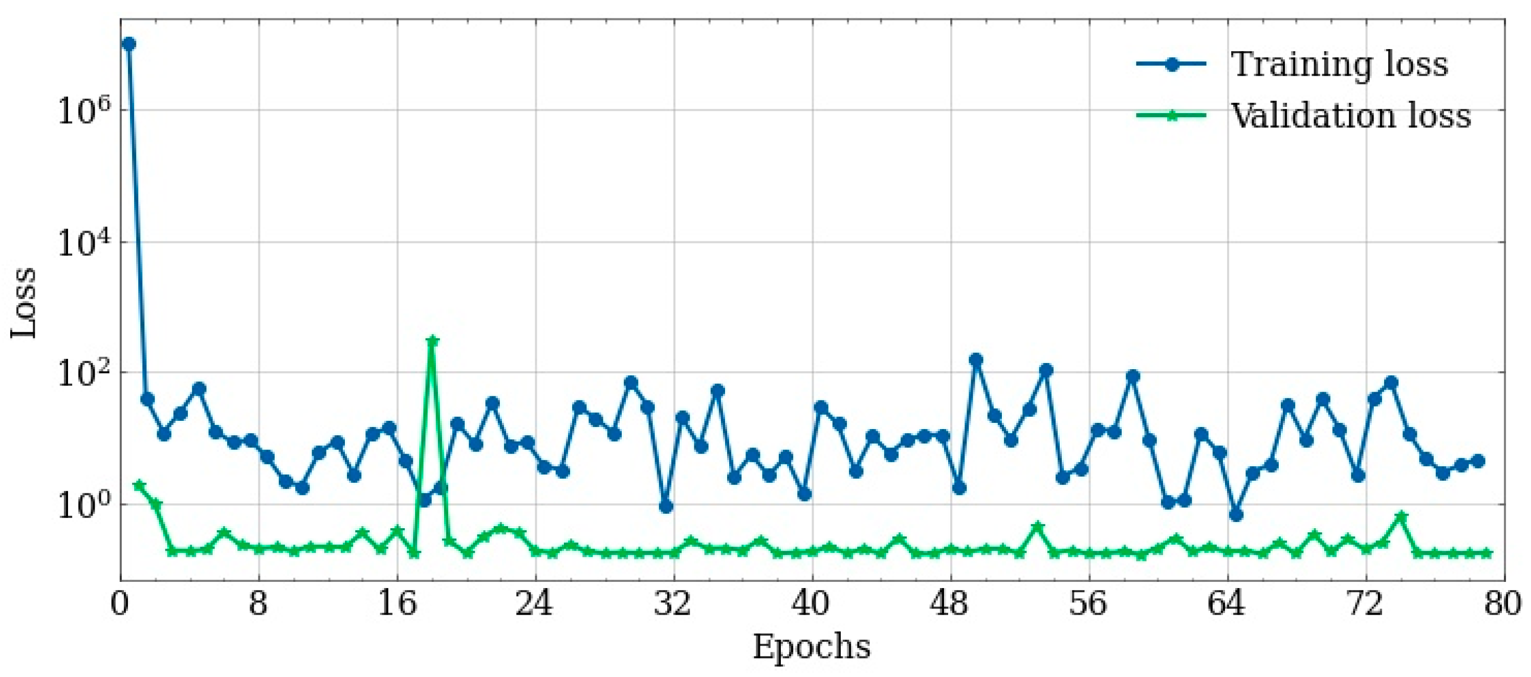
After the hyperparameters were selected, the model was retrained on the training set and verification set. The training process is shown in Figure 5.

4. Verification and Discussion

The performance of the estimator was evaluated under four friction coefficients and three vehicle speeds according to the double line change (DLC) condition of ISO3888-1 standard. Statistical quantitative indicators are given in the second part. Finally, a discussion of the results is presented.

4.1. Results

The following are the estimated results of the model proposed in this article under DLC conditions. Tests were carried out at 30 km/h, 50 km/h, and 70 km/h, followed by a comprehensive comparison of the results.

4.1.1. DLC at 30 km/h

The estimation results of DLC at 30 km/h are shown in Figure 6. The first 25 s is the left DLC condition, and the last 25 s is the right DLC condition. The figure shows that the LSTM estimator performs well at low speed.

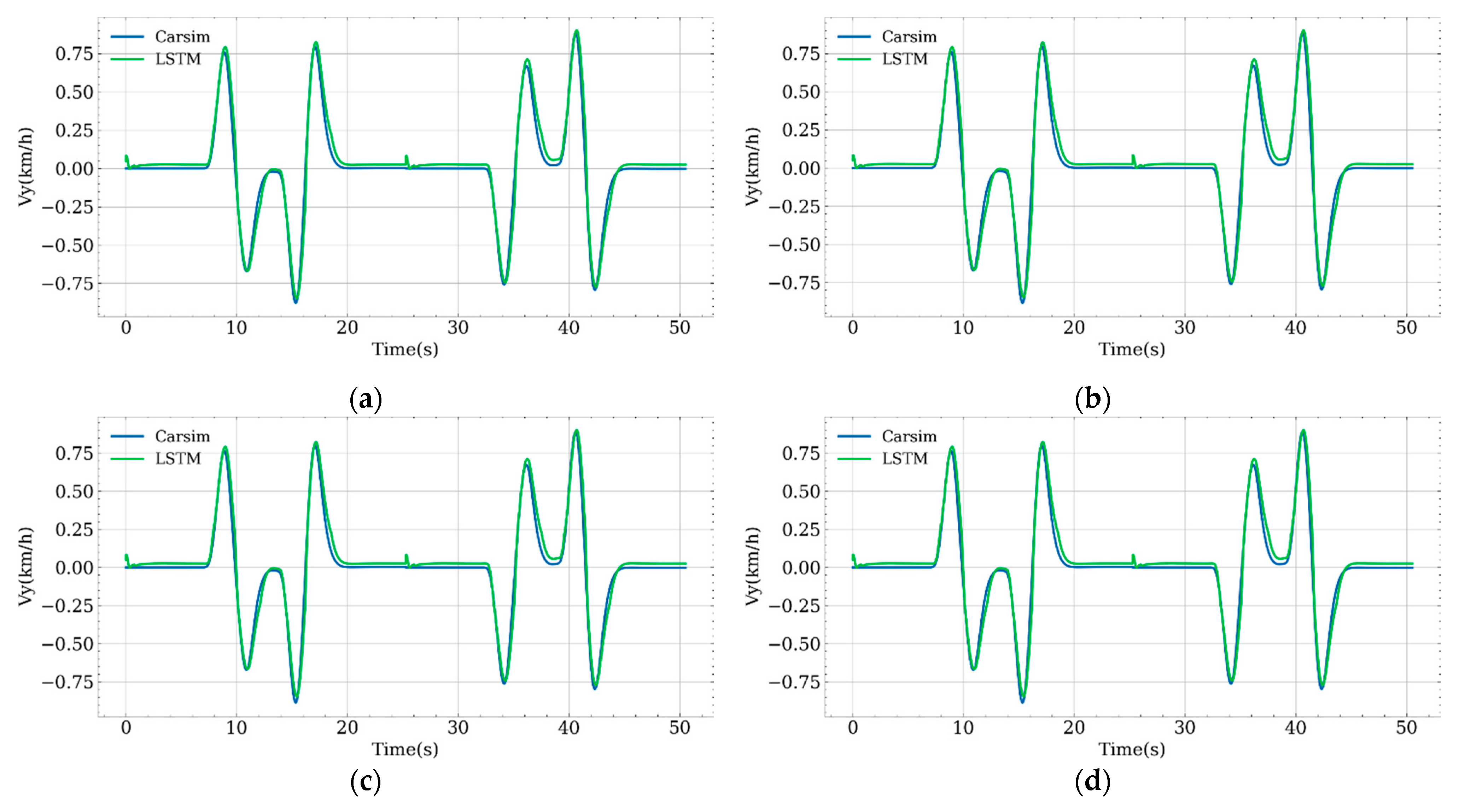
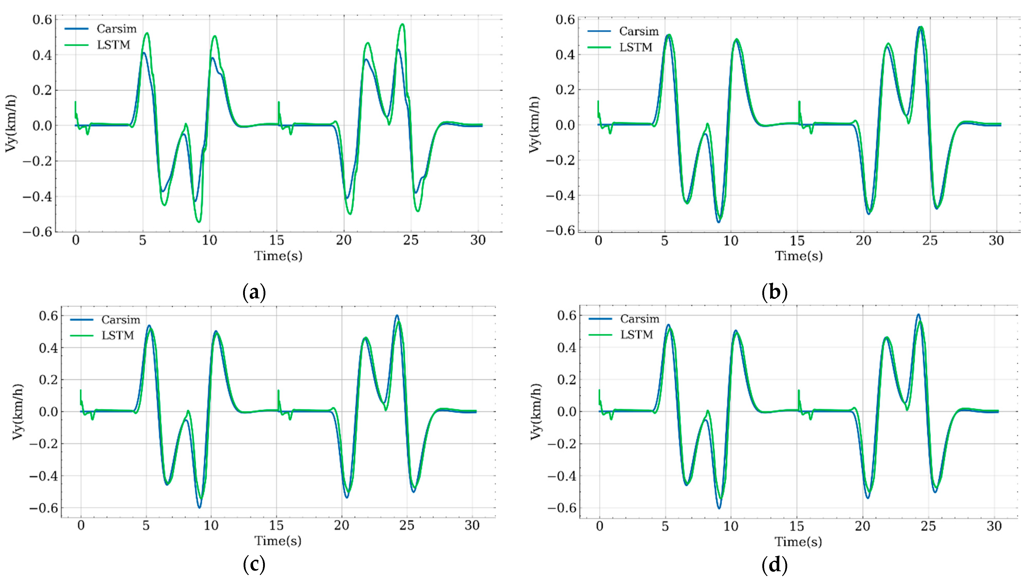
4.1.2. DLC at 50 km/h

The estimation results of DLC at 50 km/h are shown in in Figure 7. The first 15 s is the left DLC condition, and the last 15 s is the right DLC condition. It can be seen from the figure that it has good estimation performance at medium speed, and that the estimation performance changes little in the case of a change in the road friction coefficient.

4.1.3. DLC at 70 km/h

The estimation results of DLC at 70 km/h are shown in in Figure 8. The first 11 s is the left DLC condition, and the last 11 s is the right DLC condition. It can be seen that the LSTM estimator has poor performance and large relative error under high-speed conditions.

4.1.4. Comparison of the Results

At the beginning of each test, there is an obvious error in the estimated value, and then it quickly fell back to near the true value. At 30 km/h and 50 km/h, the estimated results of the proposed algorithm have a small deviation from the true value. At some moments, the result under 50 km/h has a slightly larger deviation, and these moments are mainly at the positions of wave crests and troughs. However, the test result under 70 km/h presents a large deviation from the true value.

In addition, at 70 km/h, the fluctuation trend of the true value is different from 30 km/h and 50 km/h. The true value signal tends to have four crests instead of only two crests. This is manifested when the road friction coefficient increases. However, the fluctuation trend of the estimated value is consistent with the trend at the previous two speeds, only two peaks and two troughs appear.

4.2. Quantitative Analysed Metrics

The main quantitative analysis metrics are the prediction relative to reference RMSE and MAE. RMSE and MAE are defined as:

$$RMSE=\sqrt{\frac{1}{m}{\displaystyle \sum }_{i=1}^m{\left(v_y-\widehat{v_y}\right)}^2}$$

(9)

$$MAE=\frac{1}{m}{\displaystyle \sum }_{i=1}^m\left|v_y-\widehat{v_y}\right|$$

(10)

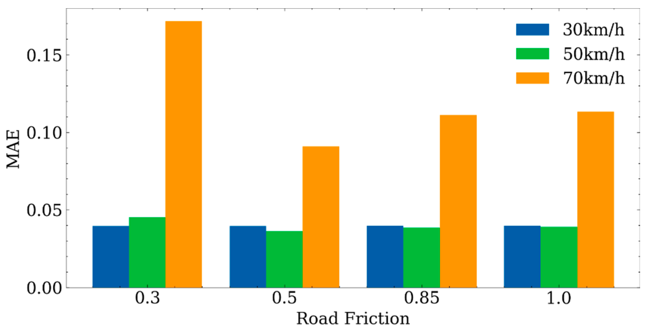
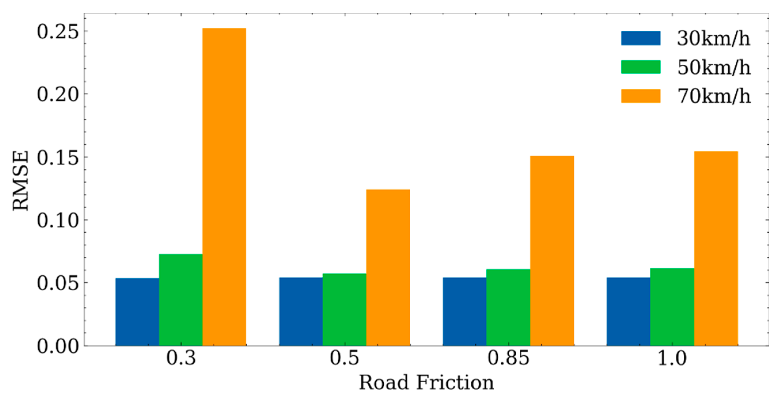
Figure 9 shows the RMSE values estimated by the method proposed in this paper under three vehicle speeds and four road friction coefficients. The RMSE value at 70 km/h is significantly higher than that at 30 km/h and 50 km/h, which indicates that this method performs well at medium and low speeds, but poorly at high speed DLC, which is consistent with the MAE value in Figure 10.

4.3. Discussion

According to the results of the previous two parts, the proposed method works well at low and medium speeds and can accurately estimate the lateral velocity. With the decrease of the road friction coefficient, the deviation of the estimated value will not change significantly, and therefore it is robust to the change of the road friction coefficient. Due to the dynamics of the vehicle itself, the fluctuation trend of the lateral velocity at high speed is significantly different from that at low and medium speeds, which leads to poor performance of the proposed method at 70 km/h. It also indicates that the proposed method has not fully learned the dynamic characteristics of the vehicle. On the one hand, this may be due to the lack of data representing the characteristics of the vehicle. On the other hand, it may be due to the model’s hypothesis space being too small to represent all vehicle dynamics characteristics.

In the real world, it is difficult for a vehicle to complete the DLC test at a higher speed while maintaining stability, so testing at higher speed is not carried out. The reason why the test is only performed under the DLC condition rather than other standard conditions is that the DLC condition is one of the most extreme conditions that can be encountered in the actual driving environment, and it is also the most common situation for vehicle stability programs to function. Having good estimation performance under DLC condition represents the superiority of the method.

Due to the black-box characteristics of deep learning, it is necessary to conduct large-scale non-parametric testing to ensure that it will not output unreasonable values under certain circumstances before applying it to safety-critical fields. This study did not conduct large-scale testing since it requires a lot of time and costs, which is also its limitation.

5. Conclusions

Aiming to resolve the problem of poor accuracy of vehicle lateral velocity estimation by traditional estimation methods, a lateral velocity estimation neural network based on LSTM is designed in this paper. Lateral velocity is an important state for vehicle stability control. As the vehicle is an inertial system, the current state is related to the previous one, whose correlation can be well manifested by LSTM. The results show that the network can accurately estimate the lateral velocity at low and medium speeds. At high speed, there is a relatively larger error. In addition, it is robust to the change of the road friction coefficient.

Future research will focus on the estimation performance at high speed. Furthermore, the estimated information is used in vehicle active control and automatic driving system to enhance the control stability and intelligence of vehicles.