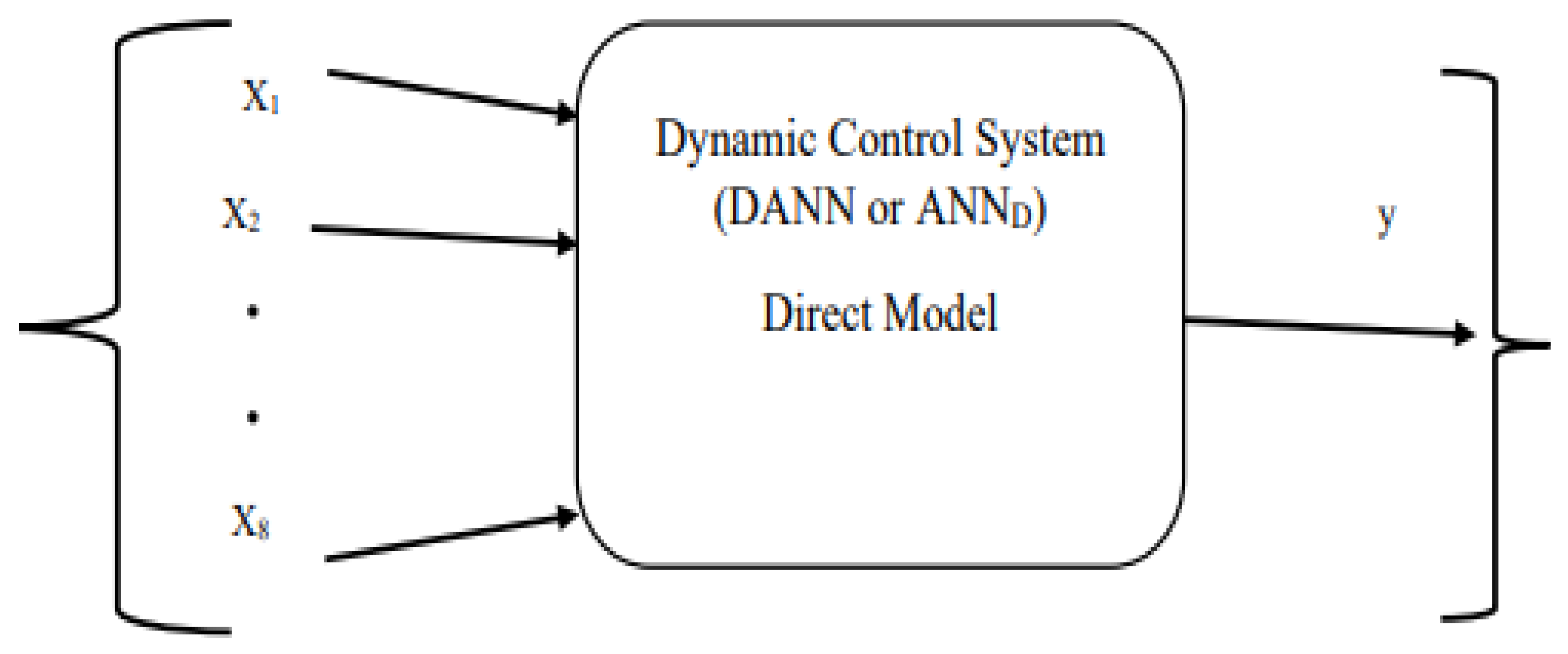
Figure 1.
Dynamic Control System for the PEVs.
Figure 1.
Dynamic Control System for the PEVs.
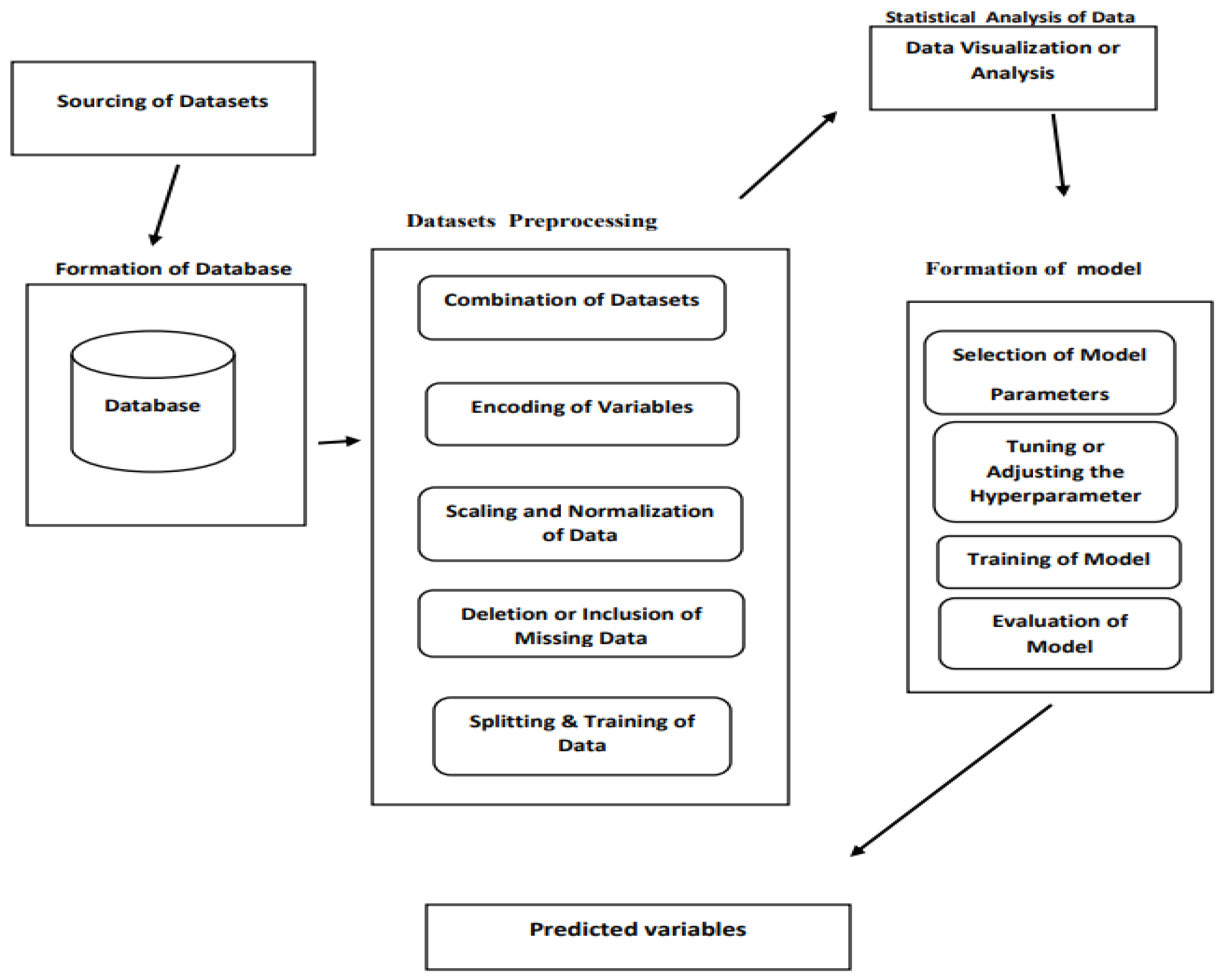
Figure 2.
Process flow for the parametric predictions.
Figure 2.
Process flow for the parametric predictions.
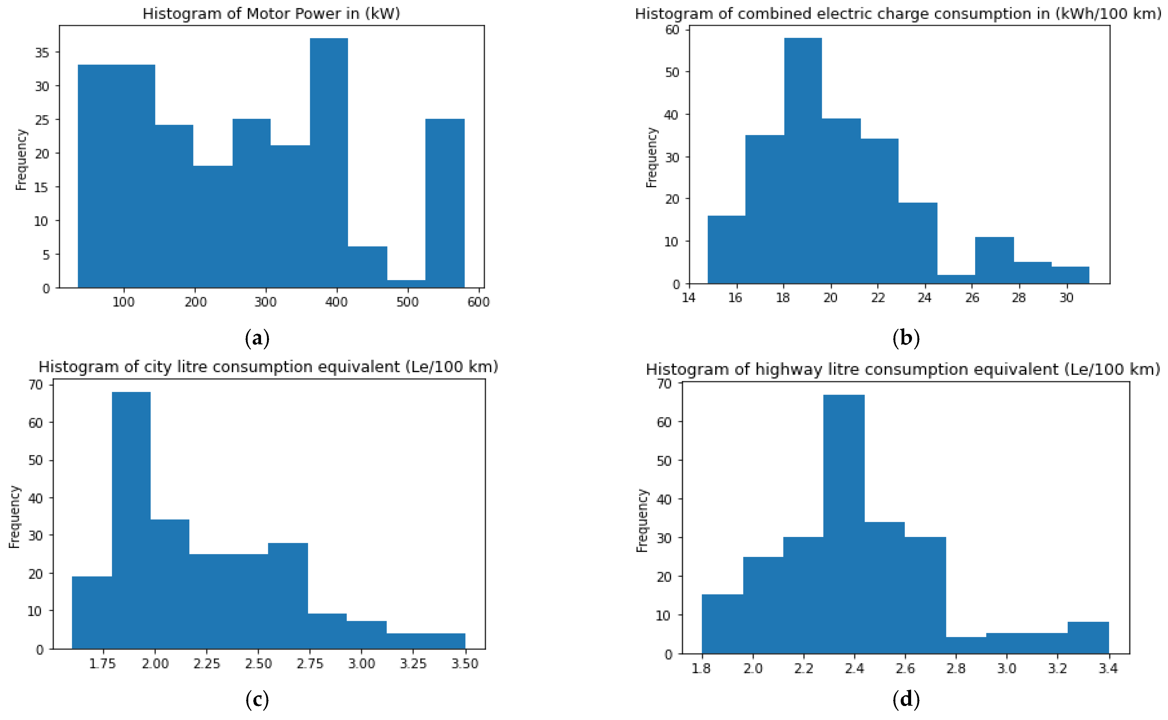
Figure 3.
Dataset visualization. (a) Motor Power; (b) Combined electric charge consumption; (c) City litre consumption equivalent; (d) Highway litre consumption equivalent; (e) Recharge Time; (f) Combined (highway and city) consumption equivalent; (g) City electric charge consumption; (h) highway electric charge consumption; (i) Range.
Figure 4.
Selected parameters for the model.
Figure 4.
Selected parameters for the model.
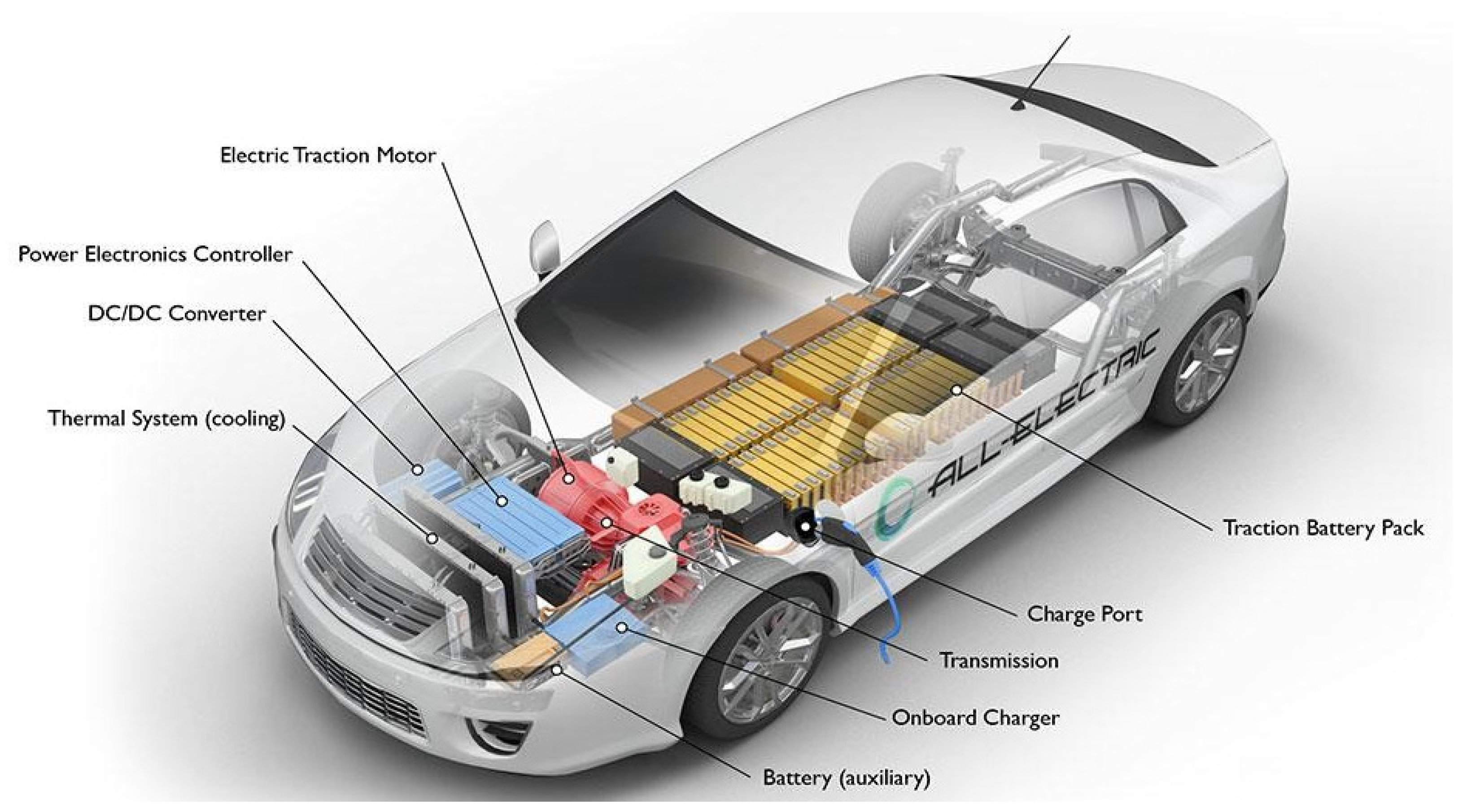
Figure 5.
Pure electric vehicle [
29].
Figure 5.
Pure electric vehicle [
29].
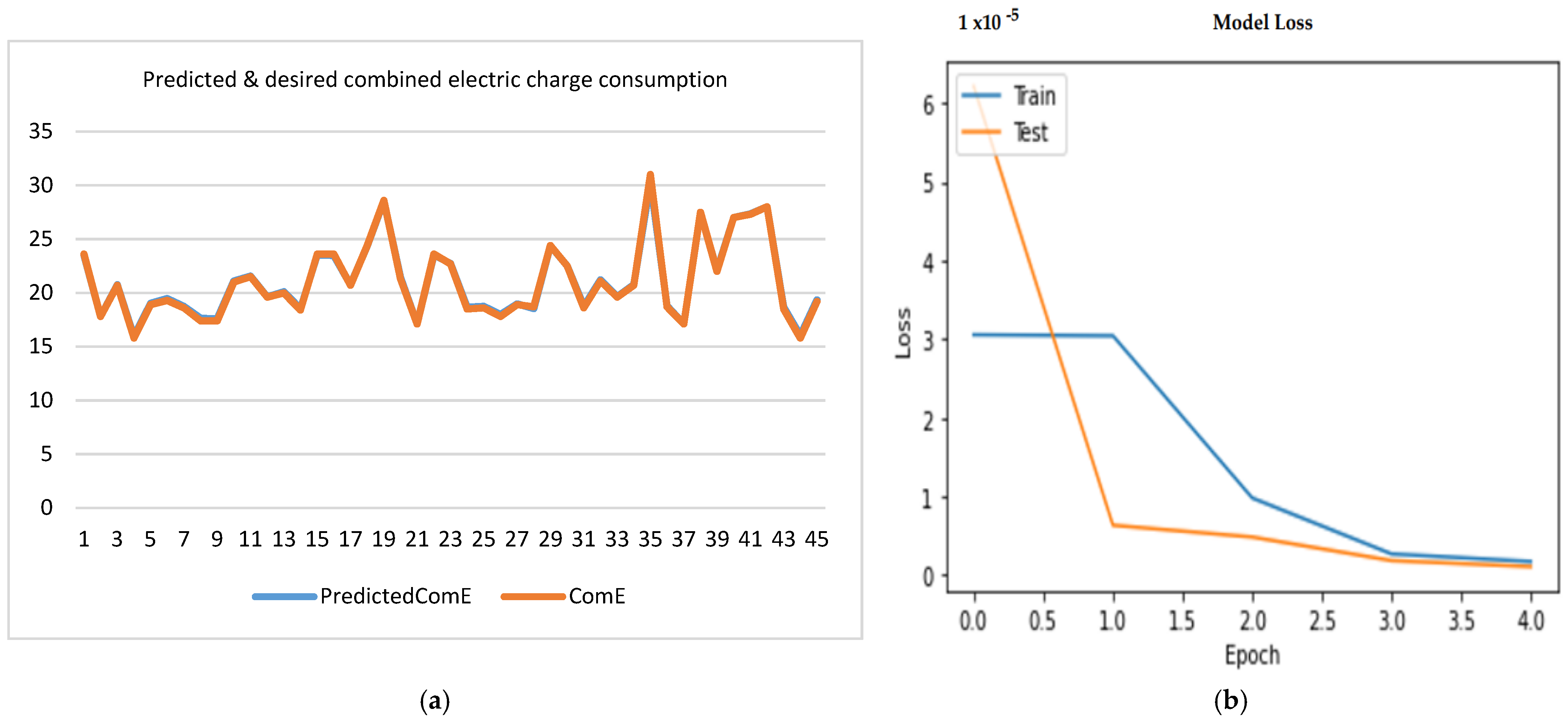
Figure 6.
Performance measurement of the combined electric charge consumption. (a) Behaviour of the combined electric charge consumption; (b) Model loss with increase in epoch.
Figure 6.
Performance measurement of the combined electric charge consumption. (a) Behaviour of the combined electric charge consumption; (b) Model loss with increase in epoch.
Figure 7.
Predicted city electric charge consumption analysis. (a) Behaviour of the city electric charge consumption; (b) Model loss with increase in epoch.
Figure 7.
Predicted city electric charge consumption analysis. (a) Behaviour of the city electric charge consumption; (b) Model loss with increase in epoch.
Figure 8.
Predicted and desired recharge time analysis. (a) Behaviour of the predicted and desired of recharge time; (b) Model loss with increase in epoch.
Figure 8.
Predicted and desired recharge time analysis. (a) Behaviour of the predicted and desired of recharge time; (b) Model loss with increase in epoch.
Figure 9.
Predicted highway electric charge consumption analysis. (a) Behaviour of the highway electric charge consumption; (b) Model loss with increase in epoch.
Figure 9.
Predicted highway electric charge consumption analysis. (a) Behaviour of the highway electric charge consumption; (b) Model loss with increase in epoch.
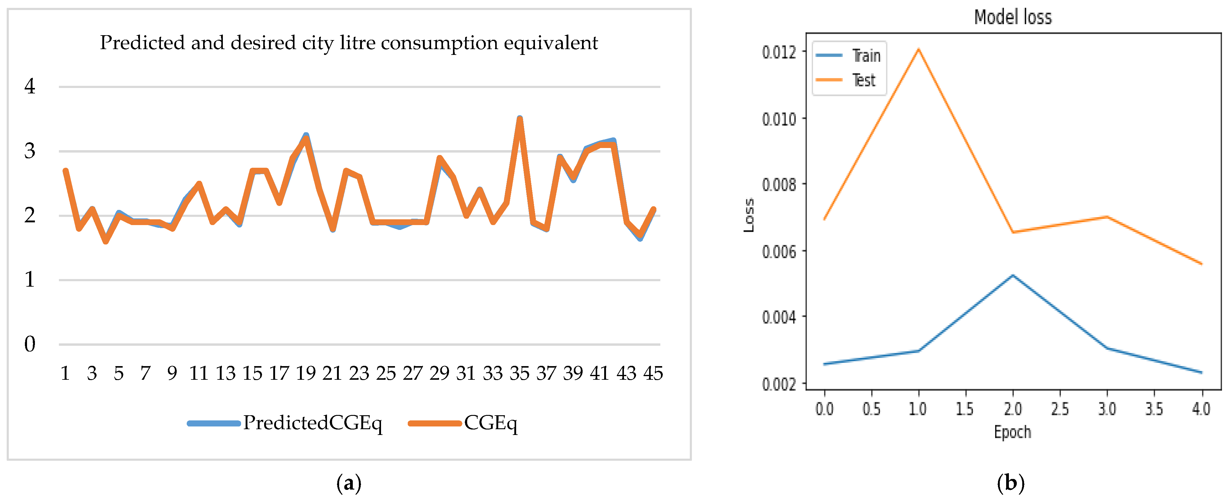
Figure 10.
City gasoline litre consumption equivalent analysis. (a) Behaviour of city gasoline litre consumption equivalent; (b) Model loss with increase in epoch.
Figure 10.
City gasoline litre consumption equivalent analysis. (a) Behaviour of city gasoline litre consumption equivalent; (b) Model loss with increase in epoch.
Figure 11.
Highway gasoline litre consumption equivalent analysis. (a) Behaviour of the highway litre consumption equivalent; (b) Model loss with increase in epoch.
Figure 11.
Highway gasoline litre consumption equivalent analysis. (a) Behaviour of the highway litre consumption equivalent; (b) Model loss with increase in epoch.
Figure 12.
Combined gasoline litre consumption equivalent analysis. (a) Behaviour of the combined litre consumption equivalent; (b) Model loss with increase in epoch.
Figure 12.
Combined gasoline litre consumption equivalent analysis. (a) Behaviour of the combined litre consumption equivalent; (b) Model loss with increase in epoch.
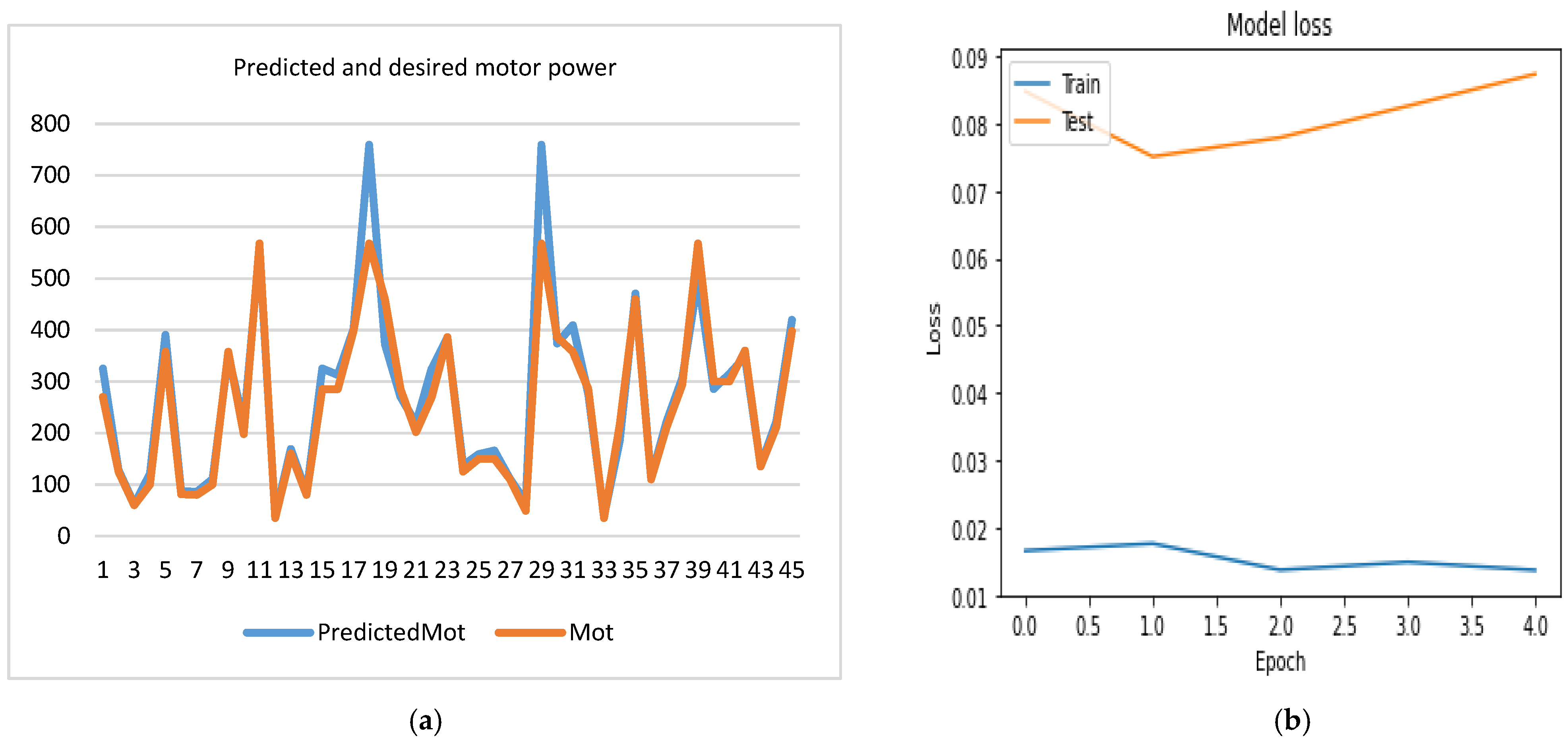
Figure 13.
Predicted electrical motor power analysis. (a) Behaviour of the predicted electrical motor power; (b) Model loss with increase in epoch.
Figure 13.
Predicted electrical motor power analysis. (a) Behaviour of the predicted electrical motor power; (b) Model loss with increase in epoch.
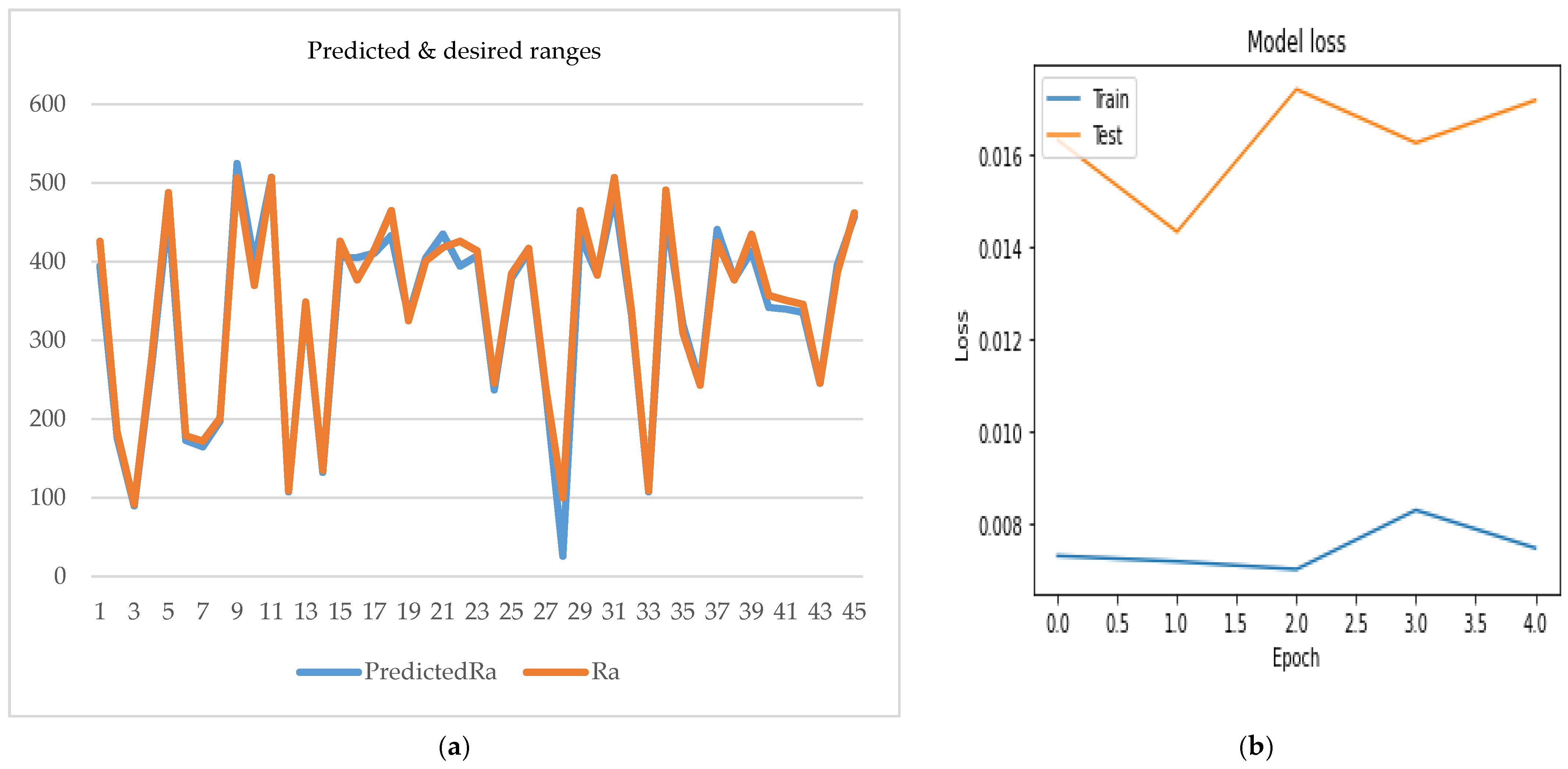
Figure 14.
Predicted range analysis. (a) Behaviour of the predicted range; (b) Model loss with increase in epoch.
Figure 14.
Predicted range analysis. (a) Behaviour of the predicted range; (b) Model loss with increase in epoch.
Figure 15.
Redefined parametric predictions performance measurement. (a) City electric charge consumption; (b) Highway electric charge consumption; (c) Combined electric charge consumption; (d) Electric motor power; (e) City gasoline litre consumption equivalent; (f) Highway gasoline litre consumption equivalent; (g) Combined gasoline litre consumption equivalent; (h) Recharge Time; (i) Range.
Figure 16.
Model evaluation with the redefined parameters.
Figure 16.
Model evaluation with the redefined parameters.
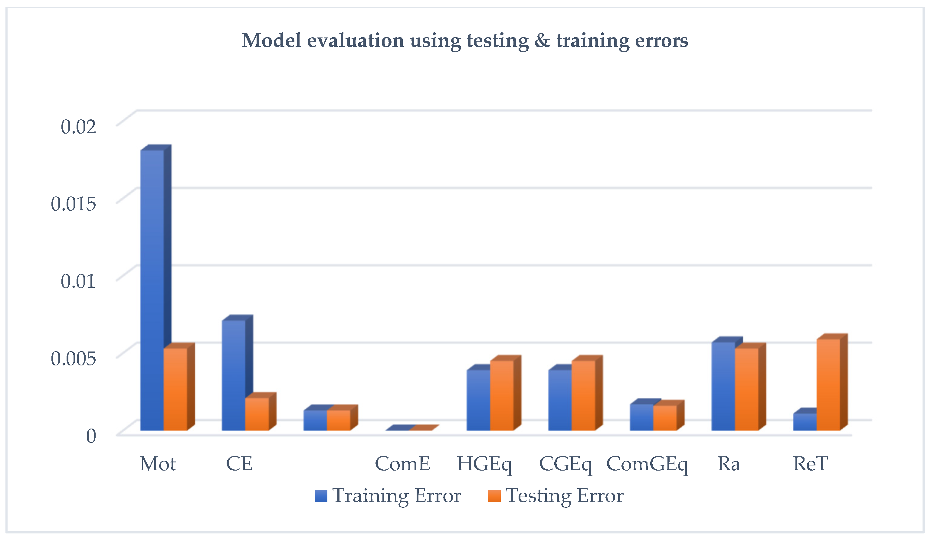
Figure 17.
Training and testing errors for the nine variables.
Figure 17.
Training and testing errors for the nine variables.
Figure 18.
Model evaluation.
Figure 18.
Model evaluation.
Table 1.
Datasets for the model.
Table 1.
Datasets for the model.
| | Year | Make | Mot | CE | HE | ComE | CGEq | HGEq | ComGEq | Ra | ReT |
|---|
| 0 | 2012 | Mitsubishi | 49 | 16.9 | 21.4 | 18.7 | 1.9 | 2.4 | 2.1 | 100 | 7 |
| 1 | 2012 | Nissan | 80 | 19.3 | 23 | 21.1 | 2.2 | 2.6 | 2.4 | 117 | 7 |
| 2 | 2013 | Ford | 107 | 19 | 21 | 20 | 2.1 | 2.4 | 2.2 | 122 | 4 |
| 3 | 2013 | Mitsubishi | 49 | 16.9 | 21.4 | 18.7 | 1.9 | 2.4 | 2.1 | 100 | 7 |
| 4 | 2013 | Nissan | 80 | 19.3 | 23 | 21.1 | 2.2 | 2.6 | 2.2 | 117 | 7 |
| 5 | 2013 | Smart | 35 | 17.2 | 22.5 | 19.6 | 1.9 | 2.5 | 2.2 | 109 | 8 |
| 6 | 2013 | Smart | 35 | 17.2 | 22.5 | 19.6 | 1.9 | 2.5 | 2.2 | 109 | 8 |
| 7 | 2013 | Tesla | 225 | 22.4 | 21.9 | 22.2 | 2.5 | 2.5 | 2.5 | 224 | 6 |
| 8 | 2013 | Tesla | 225 | 22.2 | 21.7 | 21.9 | 2.5 | 2.4 | 2.5 | 335 | 10 |
| 9 | 2013 | Tesla | 270 | 23.8 | 23.2 | 23.6 | 2.7 | 2.6 | 2.6 | 426 | 12 |
| 10 | 2013 | Tesla | 310 | 23.9 | 23.2 | 23.6 | 2.7 | 2.6 | 2.6 | 426 | 12 |
| 11 | 2014 | Chevrolet | 104 | 16 | 19.6 | 17.8 | 1.8 | 2.2 | 2 | 131 | 7 |
| 12 | 2014 | Ford | 107 | 19 | 21.1 | 20 | 2.1 | 2.4 | 2.2 | 122 | 4 |
| 13 | 2014 | Mitsubishi | 49 | 16.9 | 21.4 | 18.7 | 1.9 | 2.4 | 2.1 | 100 | 7 |
| 14 | 2014 | Nissan | 80 | 16.5 | 20.8 | 18.4 | 1.9 | 2.3 | 2.1 | 135 | 5 |
Table 2.
Prediction result at model formation.
Table 2.
Prediction result at model formation.
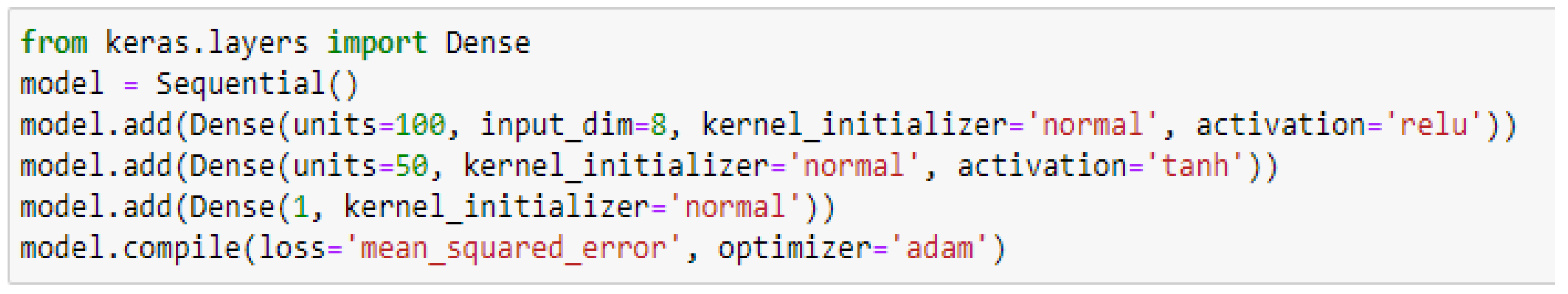
| (a) Summary of the Model |
| Model Summary |
| Layer (type) | Output Shape | Parameter # |
| Dense_33 (Dense) | (None, 100) | 900 |
| Dense_34 (Dense) | (None, 50) | 5050 |
| Dense_35 (Dense) | (None, 1) | 51 |
| Total parameters: | 6001 | |
| Total parameters: | 6001 | |
| Non-trainableparameters: | 0 | |
| (b) Predicted Combined Electric Charge Consumption |
| | CE | ReT | HE | CGEq | HGEq | ComGEq | Mot | Ra | ComE | PredictedComE |
| 0 | 23.8 | 12 | 23.2 | 2.7 | 2.6 | 2.6 | 270 | 426 | 23.6 | 23.518833 |
| 1 | 16.2 | 5 | 19.7 | 1.8 | 2.2 | 2 | 125 | 183 | 17.8 | 17.820225 |
| 2 | 18.7 | 3 | 23.1 | 2.1 | 2.6 | 2.3 | 60 | 92 | 20.7 | 20.755283 |
| 3 | 14.5 | 5.8 | 17.4 | 1.6 | 1.9 | 1.8 | 100 | 274 | 15.8 | 15.946842 |
| 4 | 18.2 | 10 | 19.8 | 2 | 2.2 | 2.1 | 358 | 488 | 18.9 | 19.017338 |
| 5 | 16.8 | 5 | 22.4 | 1.9 | 2.5 | 2.2 | 81 | 179 | 19.3 | 19.458347 |
| 6 | 17 | 6 | 20.7 | 1.9 | 2.3 | 2.1 | 80 | 172 | 18.6 | 18.737461 |
| 7 | 16.8 | 5.3 | 18.6 | 1.9 | 2.1 | 2 | 100 | 201 | 17.4 | 17.652714 |
| 8 | 16.3 | 10 | 18.7 | 1.8 | 2.1 | 2 | 358 | 507 | 17.4 | 17.585972 |
| 9 | 19.9 | 8.8 | 22.4 | 2.2 | 2.5 | 2.4 | 198 | 370 | 21 | 21.097385 |
Table 3.
Predicted and desired city electric charge consumption.
Table 3.
Predicted and desired city electric charge consumption.
| | ReT | HE | CGEq | HGEq | ComGEq | Mot | Ra | ComE | CE | Predicted CE |
|---|
| 0 | 12 | 23.2 | 2.7 | 2.6 | 2.6 | 270 | 426 | 23.6 | 23.8 | 24.129328 |
| 1 | 5 | 19.7 | 1.8 | 2.2 | 2 | 125 | 183 | 17.8 | 16.2 | 16.105284 |
| 2 | 3 | 23.1 | 2.1 | 2.6 | 2.3 | 60 | 92 | 20.7 | 18.7 | 18.772221 |
| 3 | 5.8 | 17.4 | 1.6 | 1.9 | 1.8 | 100 | 274 | 15.8 | 14.5 | 14.315234 |
| 4 | 10 | 19.8 | 2 | 2.2 | 2.1 | 358 | 488 | 18.9 | 18.2 | 18.061446 |
| 5 | 5 | 22.4 | 1.9 | 2.5 | 2.2 | 81 | 179 | 19.3 | 16.8 | 16.890638 |
| 6 | 6 | 20.7 | 1.9 | 2.3 | 2.1 | 80 | 172 | 18.6 | 17 | 16.919226 |
| 7 | 5.3 | 18.6 | 1.9 | 2.1 | 2 | 100 | 201 | 17.4 | 16.8 | 16.77796 |
| 8 | 10 | 18.7 | 1.8 | 2.1 | 2 | 358 | 507 | 17.4 | 16.3 | 16.444208 |
| 9 | 8.8 | 22.4 | 2.2 | 2.5 | 2.4 | 198 | 370 | 21 | 19.9 | 19.894707 |
Table 4.
Predicted and desired Recharge Time.
Table 4.
Predicted and desired Recharge Time.
| | HE | CGEq | HGEq | ComGEq | Mot | Ra | ComE | CE | ReT | Predicted ReT |
|---|
| 0 | 24.28 | 2.49 | 2.75 | 2.53 | 402.63 | 347.18 | 22.28 | 23.43 | 12.099 | 12.21354 |
| 1 | 17.12 | 1.96 | 2.10 | 2.068 | 135.04 | 217.75 | 16.82 | 16.55 | 6.67 | 6.568537 |
| 2 | 15.06 | 2.48 | 2.32 | 2.53 | 268.84 | 159.723 | 14.78 | 19.99 | 8.45 | 8.39825 |
| 3 | 17.93 | 1.603 | 1.95 | 1.72 | 45.847 | 195.43 | 18.87 | 14.17 | 5.45 | 5.329853 |
| 4 | 22.227 | 1.971 | 2.24 | 2.068 | 179.64 | 425.73 | 23.67 | 17.85 | 8.096 | 7.97622 |
| 5 | 17.1 | 2.37 | 2.17 | 2.41 | 224.23 | 178.468 | 16.73 | 18.32 | 7.094 | 7.096871 |
| 6 | 18.13 | 2.1 | 2.17 | 2.18 | 179.64 | 177.58 | 16.58 | 17.5 | 7.24 | 7.139585 |
| 7 | 17.42 | 1.79 | 2.17 | 1.95 | 135.04 | 195.43 | 17.22 | 16.072 | 7.09 | 7.081111 |
| 8 | 22.23 | 1.8 | 2.1 | 1.95 | 135.04 | 425.73 | 24.1 | 16.072 | 6.74 | 6.821907 |
| 9 | 20.1 | 2.37 | 2.39 | 2.41 | 313.44 | 282.9 | 21.02 | 20.34 | 9.31 | 9.131731 |
Table 5.
Predicted and desired highway electric charge consumption.
Table 5.
Predicted and desired highway electric charge consumption.
| CGEq | HGEq | ComGEq | Mot | Ra | ComE | CE | ReT | HE | Predicted
HE |
|---|
| 2.7 | 2.6 | 2.6 | 270 | 426 | 23.6 | 23.8 | 12 | 23.2 | 23.189518 |
| 1.8 | 2.2 | 2 | 125 | 183 | 17.8 | 16.2 | 5 | 19.7 | 19.625205 |
| 2.1 | 2.6 | 2.3 | 60 | 92 | 20.7 | 18.7 | 3 | 23.1 | 23.005917 |
| 1.6 | 1.9 | 1.8 | 100 | 274 | 15.8 | 14.5 | 5.8 | 17.4 | 17.441454 |
| 2 | 2.2 | 2.1 | 358 | 488 | 18.9 | 18.2 | 10 | 19.8 | 19.8613 |
| 1.9 | 2.5 | 2.2 | 81 | 179 | 19.3 | 16.8 | 5 | 22.4 | 22.27434 |
| 1.9 | 2.3 | 2.1 | 80 | 172 | 18.6 | 17 | 6 | 20.7 | 20.554855 |
| 1.9 | 2.1 | 2 | 100 | 201 | 17.4 | 16.8 | 5.3 | 18.6 | 18.633545 |
| 1.8 | 2.1 | 2 | 358 | 507 | 17.4 | 16.3 | 10 | 18.7 | 18.787008 |
| 2.2 | 2.5 | 2.4 | 198 | 370 | 21 | 19.9 | 8.8 | 22.4 | 22.373301 |
Table 6.
Predicted and desired city gasoline litre consumption equivalent.
Table 6.
Predicted and desired city gasoline litre consumption equivalent.
| | HGEq | ComGEq | Mot | Ra | ComE | CE | ReT | HE | CGEq | Predicted CGEq |
|---|
| 0 | 2.6 | 2.6 | 270 | 426 | 23.6 | 23.8 | 12 | 23.2 | 2.7 | 2.683975 |
| 1 | 2.2 | 2 | 125 | 183 | 17.8 | 16.2 | 5 | 19.7 | 1.8 | 1.821692 |
| 2 | 2.6 | 2.3 | 60 | 92 | 20.7 | 18.7 | 3 | 23.1 | 2.1 | 2.106232 |
| 3 | 1.9 | 1.8 | 100 | 274 | 15.8 | 14.5 | 5.8 | 17.4 | 1.6 | 1.604526 |
| 4 | 2.2 | 2.1 | 358 | 488 | 18.9 | 18.2 | 10 | 19.8 | 2 | 2.046841 |
| 5 | 2.5 | 2.2 | 81 | 179 | 19.3 | 16.8 | 5 | 22.4 | 1.9 | 1.91557 |
| 6 | 2.3 | 2.1 | 80 | 172 | 18.6 | 17 | 6 | 20.7 | 1.9 | 1.913931 |
| 7 | 2.1 | 2 | 100 | 201 | 17.4 | 16.8 | 5.3 | 18.6 | 1.9 | 1.85855 |
| 8 | 2.1 | 2 | 358 | 507 | 17.4 | 16.3 | 10 | 18.7 | 1.8 | 1.843146 |
| 9 | 2.5 | 2.4 | 198 | 370 | 21 | 19.9 | 8.8 | 22.4 | 2.2 | 2.259193 |
Table 7.
Predicted and desired highway gasoline litre consumption equivalent.
Table 7.
Predicted and desired highway gasoline litre consumption equivalent.
| | ComGEq | Mot | Ra | ComE | CE | ReT | HE | CGEq | HGEq | Predicted HGEq |
|---|
| 0 | 2.6 | 270 | 426 | 23.6 | 23.8 | 12 | 23.2 | 2.7 | 2.6 | 2.616106 |
| 1 | 2 | 125 | 183 | 17.8 | 16.2 | 5 | 19.7 | 1.8 | 2.2 | 2.19862 |
| 2 | 2.3 | 60 | 92 | 20.7 | 18.7 | 3 | 23.1 | 2.1 | 2.6 | 2.605645 |
| 3 | 1.8 | 100 | 274 | 15.8 | 14.5 | 5.8 | 17.4 | 1.6 | 1.9 | 1.899809 |
| 4 | 2.1 | 358 | 488 | 18.9 | 18.2 | 10 | 19.8 | 2 | 2.2 | 2.210691 |
| 5 | 2.2 | 81 | 179 | 19.3 | 16.8 | 5 | 22.4 | 1.9 | 2.5 | 2.21091 |
| 6 | 2.1 | 80 | 172 | 18.6 | 17 | 6 | 20.7 | 1.9 | 2.3 | 2.523738 |
| 7 | 2 | 100 | 201 | 17.4 | 16.8 | 5.3 | 18.6 | 1.9 | 2.1 | 2.313696 |
| 8 | 2 | 358 | 507 | 17.4 | 16.3 | 10 | 18.7 | 1.8 | 2.1 | 2.072292 |
| 9 | 2.4 | 198 | 370 | 21 | 19.9 | 8.8 | 22.4 | 2.2 | 2.5 | 2.484709 |
Table 8.
Predicted and desired combined gasoline litre consumption equivalent.
Table 8.
Predicted and desired combined gasoline litre consumption equivalent.
| | Mot | Ra | ComE | CE | ReT | HE | CGEq | HGEq | ComGEq | Predicted ComGEq |
|---|
| 0 | 270 | 426 | 23.6 | 23.8 | 12 | 23.2 | 2.7 | 2.6 | 2.6 | 2.59812 |
| 1 | 125 | 183 | 17.8 | 16.2 | 5 | 19.7 | 1.8 | 2.2 | 2 | 2.02092 |
| 2 | 60 | 92 | 20.7 | 18.7 | 3 | 23.1 | 2.1 | 2.6 | 2.3 | 2.305117 |
| 3 | 100 | 274 | 15.8 | 14.5 | 5.8 | 17.4 | 1.6 | 1.9 | 1.8 | 1.796104 |
| 4 | 358 | 488 | 18.9 | 18.2 | 10 | 19.8 | 2 | 2.2 | 2.1 | 2.140992 |
| 5 | 81 | 179 | 19.3 | 16.8 | 5 | 22.4 | 1.9 | 2.5 | 2.2 | 2.197978 |
| 6 | 80 | 172 | 18.6 | 17 | 6 | 20.7 | 1.9 | 2.3 | 2.1 | 2.11947 |
| 7 | 100 | 201 | 17.4 | 16.8 | 5.3 | 18.6 | 1.9 | 2.1 | 2 | 1.998774 |
| 8 | 358 | 507 | 17.4 | 16.3 | 10 | 18.7 | 1.8 | 2.1 | 2 | 1.95528 |
| 9 | 198 | 370 | 21 | 19.9 | 8.8 | 22.4 | 2.2 | 2.5 | 2.4 | 2.36263 |
Table 9.
Predicted and desired electrical motor power.
Table 9.
Predicted and desired electrical motor power.
| | Ra | ComE | CE | ReT | HE | CGEq | HGEq | ComGEq | Mot | Predicted Mot |
|---|
| 0 | 426 | 23.6 | 23.8 | 12 | 23.2 | 2.7 | 2.6 | 2.6 | 270 | 325.39328 |
| 1 | 183 | 17.8 | 16.2 | 5 | 19.7 | 1.8 | 2.2 | 2 | 125 | 127.758652 |
| 2 | 92 | 20.7 | 18.7 | 3 | 23.1 | 2.1 | 2.6 | 2.3 | 60 | 61.349003 |
| 3 | 274 | 15.8 | 14.5 | 5.8 | 17.4 | 1.6 | 1.9 | 1.8 | 100 | 121.266022 |
| 4 | 488 | 18.9 | 18.2 | 10 | 19.8 | 2 | 2.2 | 2.1 | 358 | 390.781677 |
| 5 | 179 | 19.3 | 16.8 | 5 | 22.4 | 1.9 | 2.5 | 2.2 | 81 | 87.229782 |
| 6 | 172 | 18.6 | 17 | 6 | 20.7 | 1.9 | 2.3 | 2.1 | 80 | 86.093201 |
| 7 | 201 | 17.4 | 16.8 | 5.3 | 18.6 | 1.9 | 2.1 | 2 | 100 | 110.93045 |
| 8 | 507 | 17.4 | 16.3 | 10 | 18.7 | 1.8 | 2.1 | 2 | 358 | 350.521454 |
| 9 | 370 | 21 | 19.9 | 8.8 | 22.4 | 2.2 | 2.5 | 2.4 | 198 | 218.790649 |
Table 10.
Predicted and desired ranges.
Table 10.
Predicted and desired ranges.
| | ComE | CE | ReT | HE | CGEq | HGEq | ComGEq | Mot | Ra | Predicted Ra |
|---|
| 0 | 23.6 | 23.8 | 12 | 23.2 | 2.7 | 2.6 | 2.6 | 270 | 426 | 394.53876 |
| 1 | 17.8 | 16.2 | 5 | 19.7 | 1.8 | 2.2 | 2 | 125 | 183 | 176.96542 |
| 2 | 20.7 | 18.7 | 3 | 23.1 | 2.1 | 2.6 | 2.3 | 60 | 92 | 89.903847 |
| 3 | 15.8 | 14.5 | 5.8 | 17.4 | 1.6 | 1.9 | 1.8 | 100 | 274 | 263.87628 |
| 4 | 18.9 | 18.2 | 10 | 19.8 | 2 | 2.2 | 2.1 | 358 | 488 | 463.54578 |
| 5 | 19.3 | 16.8 | 5 | 22.4 | 1.9 | 2.5 | 2.2 | 81 | 179 | 172.93135 |
| 6 | 18.6 | 17 | 6 | 20.7 | 1.9 | 2.3 | 2.1 | 80 | 172 | 164.85034 |
| 7 | 17.4 | 16.8 | 5.3 | 18.6 | 1.9 | 2.1 | 2 | 100 | 201 | 197.63403 |
| 8 | 17.4 | 16.3 | 10 | 18.7 | 1.8 | 2.1 | 2 | 358 | 507 | 524.77155 |
| 9 | 21 | 19.9 | 8.8 | 22.4 | 2.2 | 2.5 | 2.4 | 198 | 370 | 399.02506 |
Table 11.
Redefined parametric predictions.
Table 11.
Redefined parametric predictions.
| (a) City electric charge consumption |
| | HE | ComE | Mot | Ra | CGEq | HGEq | ComGEq | ReT | CE | Predicted CE |
| 0 | 23.2 | 23.6 | 270 | 426 | 2.7 | 2.6 | 2.6 | 12 | 46.6 | 47.066566 |
| 1 | 19.7 | 17.8 | 125 | 183 | 1.8 | 2.2 | 2 | 5 | 31.4 | 31.082979 |
| 2 | 23.1 | 20.7 | 60 | 92 | 2.1 | 2.6 | 2.3 | 3 | 36.4 | 36.024353 |
| 3 | 17.4 | 15.8 | 100 | 274 | 1.6 | 1.9 | 1.8 | 5.8 | 28 | 27.530424 |
| 4 | 19.8 | 18.9 | 358 | 488 | 2 | 2.2 | 2.1 | 10 | 35.4 | 34.879467 |
| 5 | 22.4 | 19.3 | 81 | 179 | 1.9 | 2.5 | 2.2 | 5 | 32.6 | 32.706402 |
| 6 | 20.7 | 18.6 | 80 | 172 | 1.9 | 2.3 | 2 | 6 | 33 | 32.533249 |
| 7 | 18.6 | 17.4 | 100 | 201 | 1.9 | 2.1 | 2 | 5.3 | 32.6 | 31.684757 |
| 8 | 22.3 | 17.4 | 358 | 507 | 1.9 | 2.1 | 2.4 | 10 | 31.6 | 31.951500 |
| 9 | 20 | 21 | 198 | 370 | 1.8 | 2.5 | 2.4 | 8.8 | 38.8 | 38.254368 |
| (b) Highway electric charge consumption |
| | CE | ComE | Mot | Ra | CGEq | HGEq | ComGEq | ReT | HE | Predicted HE |
| 0 | 23.8 | 23.6 | 270 | 426 | 2.7 | 2.6 | 2.6 | 12 | 23.2 | 23.21851 |
| 1 | 16.2 | 17.8 | 125 | 183 | 1.8 | 2.2 | 2 | 5 | 19.7 | 19.406933 |
| 2 | 18.7 | 20.7 | 60 | 92 | 2.1 | 2.6 | 2.3 | 3 | 23.1 | 23.057276 |
| 3 | 14.5 | 15.8 | 100 | 274 | 1.6 | 1.9 | 1.8 | 5.8 | 17.4 | 17.038816 |
| 4 | 18.2 | 18.9 | 358 | 488 | 2 | 2.2 | 2.1 | 10 | 19.8 | 19.505558 |
| 5 | 16.8 | 19.3 | 81 | 179 | 1.9 | 2.5 | 2.2 | 5 | 22.4 | 22.123541 |
| 6 | 17 | 18.6 | 80 | 172 | 1.9 | 2.3 | 2 | 6 | 20.7 | 20.51317 |
| 7 | 16.8 | 17.4 | 100 | 201 | 1.9 | 2.1 | 2 | 5.3 | 18.6 | 18.596674 |
| 8 | 16.3 | 17.4 | 358 | 507 | 1.9 | 2.1 | 2.4 | 10 | 18.7 | 18.57807 |
| 9 | 19.9 | 21 | 198 | 370 | 1.8 | 2.5 | 2.4 | 8.8 | 22.4 | 22.484404 |
| (c) Electric motor power |
| | HE | ReT | CGEq | HGEq | ComGEq | Ra | CE | ComE | Mot | Predicted Mot |
| 0 | 23.2 | 12 | 2.7 | 2.6 | 2.6 | 426 | 23.8 | 23.6 | 140 | 200.348709 |
| 1 | 19.7 | 5 | 1.8 | 2.2 | 2 | 183 | 16.2 | 17.8 | 67.5 | 61.672386 |
| 2 | 23.1 | 3 | 2.1 | 2.6 | 2.3 | 92 | 18.7 | 20.7 | 35 | 31.928759 |
| 3 | 17.4 | 5.8 | 1.6 | 1.9 | 1.8 | 274 | 14.5 | 15.8 | 55 | 63.545692 |
| 4 | 19.8 | 10 | 2 | 2.2 | 2.1 | 488 | 18.2 | 18.9 | 184 | 189.540115 |
| 5 | 22.4 | 5 | 1.9 | 2.5 | 2.2 | 179 | 16.8 | 19.3 | 45.5 | 46.0271 |
| 6 | 20.7 | 6 | 1.9 | 2.3 | 2 | 172 | 17 | 18.6 | 45 | 44.363953 |
| 7 | 18.6 | 5.3 | 1.9 | 2.1 | 2 | 201 | 16.8 | 17.4 | 55 | 56.778175 |
| 8 | 18.7 | 10 | 1.8 | 2.1 | 2.4 | 507 | 16.3 | 17.4 | 184 | 156.964767 |
| 9 | 22.4 | 8.8 | 2.2 | 2.5 | 2.4 | 370 | 19.9 | 21 | 104 | 124.466232 |
| (d) City gasoline litre consumption equivalent |
| | HE | HGEq | ReT | CE | ComE | Mot | Ra | ComGEq | CGEq | Predicted CGEq |
| 0 | 23.2 | 2.6 | 12 | 23.8 | 23.6 | 270 | 426 | 2.6 | 15.29 | 15.02135181 |
| 1 | 19.7 | 2.2 | 5 | 16.2 | 17.8 | 125 | 183 | 2 | 11.24 | 11.35358334 |
| 2 | 23.1 | 2.6 | 3 | 18.7 | 20.7 | 60 | 92 | 2.3 | 12.41 | 12.51209927 |
| 3 | 17.4 | 1.9 | 5.8 | 14.5 | 15.8 | 100 | 274 | 1.8 | 10.56 | 10.59348011 |
| 4 | 19.8 | 2.2 | 10 | 18.2 | 18.9 | 358 | 488 | 2.1 | 12 | 12.15197659 |
| 5 | 22.4 | 2.5 | 5 | 16.8 | 19.3 | 81 | 179 | 2.2 | 11.61 | 11.71028996 |
| 6 | 20.7 | 2.3 | 6 | 17 | 18.6 | 80 | 172 | 2 | 11.61 | 11.59972286 |
| 7 | 18.6 | 2.1 | 5.3 | 16.8 | 17.4 | 100 | 201 | 2 | 11.61 | 11.36447811 |
| 8 | 18.7 | 2.1 | 10 | 16.3 | 17.4 | 358 | 507 | 2.4 | 11.24 | 11.49509335 |
| 9 | 22.4 | 2.5 | 8.8 | 19.9 | 21 | 198 | 370 | 2.4 | 12.84 | 12.95093346 |
| (e) Highway gasoline litre consumption equivalent |
| | HE | ReT | CE | ComE | Mot | Ra | ComGEq | CGEq | HGEq | Predicted HGEq |
| 0 | 23.2 | 12 | 23.8 | 23.6 | 270 | 426 | 2.6 | 2.7 | 17.576 | 17.74665260 |
| 1 | 19.7 | 5 | 16.2 | 17.8 | 125 | 183 | 2 | 1.8 | 10.648 | 10.65536785 |
| 2 | 23.1 | 3 | 18.7 | 20.7 | 60 | 92 | 2.3 | 2.1 | 17.576 | 18.37563324 |
| 3 | 17.4 | 5.8 | 14.5 | 15.8 | 100 | 274 | 1.8 | 1.6 | 6.859 | 7.435733795 |
| 4 | 19.8 | 10 | 18.2 | 18.9 | 358 | 488 | 2.1 | 2 | 10.648 | 10.56519318 |
| 5 | 22.4 | 5 | 16.8 | 19.3 | 81 | 179 | 2.2 | 1.9 | 15.625 | 15.85181236 |
| 6 | 20.7 | 6 | 17 | 18.6 | 80 | 172 | 2 | 1.9 | 12.167 | 12.52617073 |
| 7 | 18.6 | 5.3 | 16.8 | 17.4 | 100 | 201 | 2 | 1.9 | 9.261 | 9.117634773 |
| 8 | 18.7 | 10 | 16.3 | 17.4 | 358 | 507 | 2.4 | 1.8 | 9.261 | 9.006069183 |
| 9 | 22.4 | 8.8 | 19.9 | 21 | 198 | 370 | 2.4 | 2.2 | 15.625 | 15.56515598 |
| (f) Combined gasoline litre consumption equivalent |
| | HE | ReT | CE | ComE | Mot | Ra | CGEq | HGEq | ComGEq | Predicted ComGEq |
| 0 | 23.2 | 12 | 23.8 | 23.6 | 270 | 426 | 2.7 | 2.6 | 15.52 | 16.26508331 |
| 1 | 19.7 | 5 | 16.2 | 17.8 | 125 | 183 | 1.8 | 2.2 | 10 | 9.779075623 |
| 2 | 23.1 | 3 | 18.7 | 20.7 | 60 | 92 | 2.1 | 2.6 | 12.58 | 12.86681652 |
| 3 | 17.4 | 5.8 | 14.5 | 15.8 | 100 | 274 | 1.6 | 1.9 | 8.48 | 8.135276794 |
| 4 | 19.8 | 10 | 18.2 | 18.9 | 358 | 488 | 2 | 2.2 | 10.82 | 11.03121662 |
| 5 | 22.4 | 5 | 16.8 | 19.3 | 81 | 179 | 1.9 | 2.5 | 11.68 | 11.22401524 |
| 6 | 20.7 | 6 | 17 | 18.6 | 80 | 172 | 1.9 | 2.3 | 10.82 | 10.58418751 |
| 7 | 18.6 | 5.3 | 16.8 | 17.4 | 100 | 201 | 1.9 | 2.1 | 10 | 9.605104446 |
| 8 | 18.7 | 10 | 16.3 | 17.4 | 358 | 507 | 1.8 | 2.1 | 10 | 9.768924713 |
| 9 | 22.4 | 8.8 | 19.9 | 21 | 198 | 370 | 2.2 | 2.5 | 13.52 | 12.71550655 |
| (g) Recharge time |
| | HE | ComGEq | CE | ComE | Mot | Ra | CGEq | HGEq | ReT | Predicted ReT |
| 0 | 23.2 | 2.6 | 23.8 | 23.6 | 270 | 426 | 2.7 | 2.6 | 19 | 18.99589539 |
| 1 | 19.7 | 2 | 16.2 | 17.8 | 125 | 183 | 1.8 | 2.2 | 5 | 5.247741699 |
| 2 | 23.1 | 2.3 | 18.7 | 20.7 | 60 | 92 | 2.1 | 2.6 | 1 | 1.816795230 |
| 3 | 17.4 | 1.8 | 14.5 | 15.8 | 100 | 274 | 1.6 | 1.9 | 6.6 | 6.215961456 |
| 4 | 19.8 | 2.1 | 18.2 | 18.9 | 358 | 488 | 2 | 2.2 | 15 | 15.38726711 |
| 5 | 22.4 | 2.2 | 16.8 | 19.3 | 81 | 179 | 1.9 | 2.5 | 5 | 5.549118042 |
| 6 | 20.7 | 2 | 17 | 18.6 | 80 | 172 | 1.9 | 2.3 | 7 | 7.311823845 |
| 7 | 18.6 | 2 | 16.8 | 17.4 | 100 | 201 | 1.9 | 2.1 | 5.6 | 5.555485725 |
| 8 | 18.7 | 2.4 | 16.3 | 17.4 | 358 | 507 | 1.8 | 2.1 | 15 | 14.07801914 |
| 9 | 22.4 | 2.4 | 19.9 | 21 | 198 | 370 | 2.2 | 2.5 | 12.6 | 9.335071564 |
| (h) Range |
| | HE | ComGEq | CE | ComE | Mot | ReT | CGEq | HGEq | Ra | Predicted Ra |
| 0 | 23.2 | 2.6 | 23.8 | 23.6 | 270 | 12 | 2.7 | 2.6 | 260.6 | 247.2724609 |
| 1 | 19.7 | 2 | 16.2 | 17.8 | 125 | 5 | 1.8 | 2.2 | 114.8 | 105.6697540 |
| 2 | 23.1 | 2.3 | 18.7 | 20.7 | 60 | 3 | 2.1 | 2.6 | 60.2 | 66.36408997 |
| 3 | 17.4 | 1.8 | 14.5 | 15.8 | 100 | 5.8 | 1.6 | 1.9 | 169.4 | 155.8714142 |
| 4 | 19.8 | 2.1 | 18.2 | 18.9 | 358 | 10 | 2 | 2.2 | 297.8 | 299.7419739 |
| 5 | 22.4 | 2.2 | 16.8 | 19.3 | 81 | 5 | 1.9 | 2.5 | 112.4 | 108.7931900 |
| 6 | 20.7 | 2 | 17 | 18.6 | 80 | 6 | 1.9 | 2.3 | 108.2 | 91.59775543 |
| 7 | 18.6 | 2 | 16.8 | 17.4 | 100 | 5.3 | 1.9 | 2.1 | 125.6 | 120.0908890 |
| 8 | 18.7 | 2.4 | 16.3 | 17.4 | 358 | 10 | 1.8 | 2.1 | 309.2 | 336.3500977 |
| 9 | 22.4 | 2.4 | 19.9 | 21 | 198 | 8.8 | 2.2 | 2.5 | 227 | 246.8524475 |
| (i) Combined electric charge consumption |
| | HE | ReT | CGEq | HGEq | ComGEq | Mot | Ra | CE | ComE | Predicted ComE |
| 0 | 23.2 | 12 | 2.7 | 2.6 | 2.6 | 270 | 260.6 | 23.8 | 60.8 | 60.34340286 |
| 1 | 19.7 | 5 | 1.8 | 2.2 | 2 | 125 | 114.8 | 16.2 | 43.4 | 43.52837372 |
| 2 | 23.1 | 3 | 2.1 | 2.6 | 2.3 | 60 | 60.2 | 18.7 | 52.1 | 51.92724609 |
| 3 | 17.4 | 5.8 | 1.6 | 1.9 | 1.8 | 100 | 169.4 | 14.5 | 37.4 | 37.66779327 |
| 4 | 19.8 | 10 | 2 | 2.2 | 2.1 | 358 | 297.8 | 18.2 | 46.7 | 46.68238449 |
| 5 | 22.4 | 5 | 1.9 | 2.5 | 2.2 | 81 | 112.4 | 16.8 | 47.9 | 47.92834473 |
| 6 | 20.7 | 6 | 1.9 | 2.3 | 2 | 80 | 108.2 | 17 | 45.8 | 45.81203461 |
| 7 | 18.6 | 5.3 | 1.9 | 2.1 | 2 | 100 | 125.6 | 16.8 | 42.2 | 42.57527161 |
| 8 | 18.7 | 10 | 1.8 | 2.1 | 2.4 | 358 | 309.2 | 16.3 | 42.2 | 42.24062347 |
| 9 | 22.4 | 8.8 | 2.2 | 2.5 | 2.4 | 198 | 227 | 19.9 | 53 | 52.74155426 |
Table 12.
Model evaluation using redefined parameters.
Table 12.
Model evaluation using redefined parameters.
| Parameter | MAE | MSE | RMSE |
|---|
| CGEq | 0.06405 | 0.0082 | 0.0910 |
| HGEq | 0.09516 | 0.02277 | 0.15089 |
| ComGEq | 0.1136 | 0.02266 | 0.1505 |
| ReT | 0.2449 | 0.1192 | 0.3454 |
| CE | 0.0592 | 0.004590 | 0.06774 |
| HE | 0.06426 | 0.006881 | 0.08295 |
| ComE | 0.03567 | 0.003285 | 0.05732 |
| Ra | 0.20494 | 0.05750 | 0.2398 |
| Mot | 0.3191 | 0.2073 | 0.4553 |
Table 13.
Training and testing errors.
Table 13.
Training and testing errors.
| Parameters | Training Errors | Testing Errors |
|---|
| Mot | 0.0181 | 0.0053 |
| CE | 0.0071 | 0.0021 |
| HE | 0.0013 | 0.0013 |
| ComE | 3.9132 × 10⁻⁶ | 9.698 × 10⁻⁷ |
| HGEq | 0.0039 | 0.0045 |
| CGEq | 0.0039 | 0.0045 |
| ComGEq | 0.0017 | 0.0016 |
| Ra | 0.0057 | 0.0053 |
| ReT | 0.0011 | 0.0058932 |


