
Comparisons of Real-World Vehicle Energy Efficiency with Dynamometer-Based Ratings and Simulation Models

 , ,
, ,
Abstract
:1. Introduction
2. Real-World Vehicles Trip Data
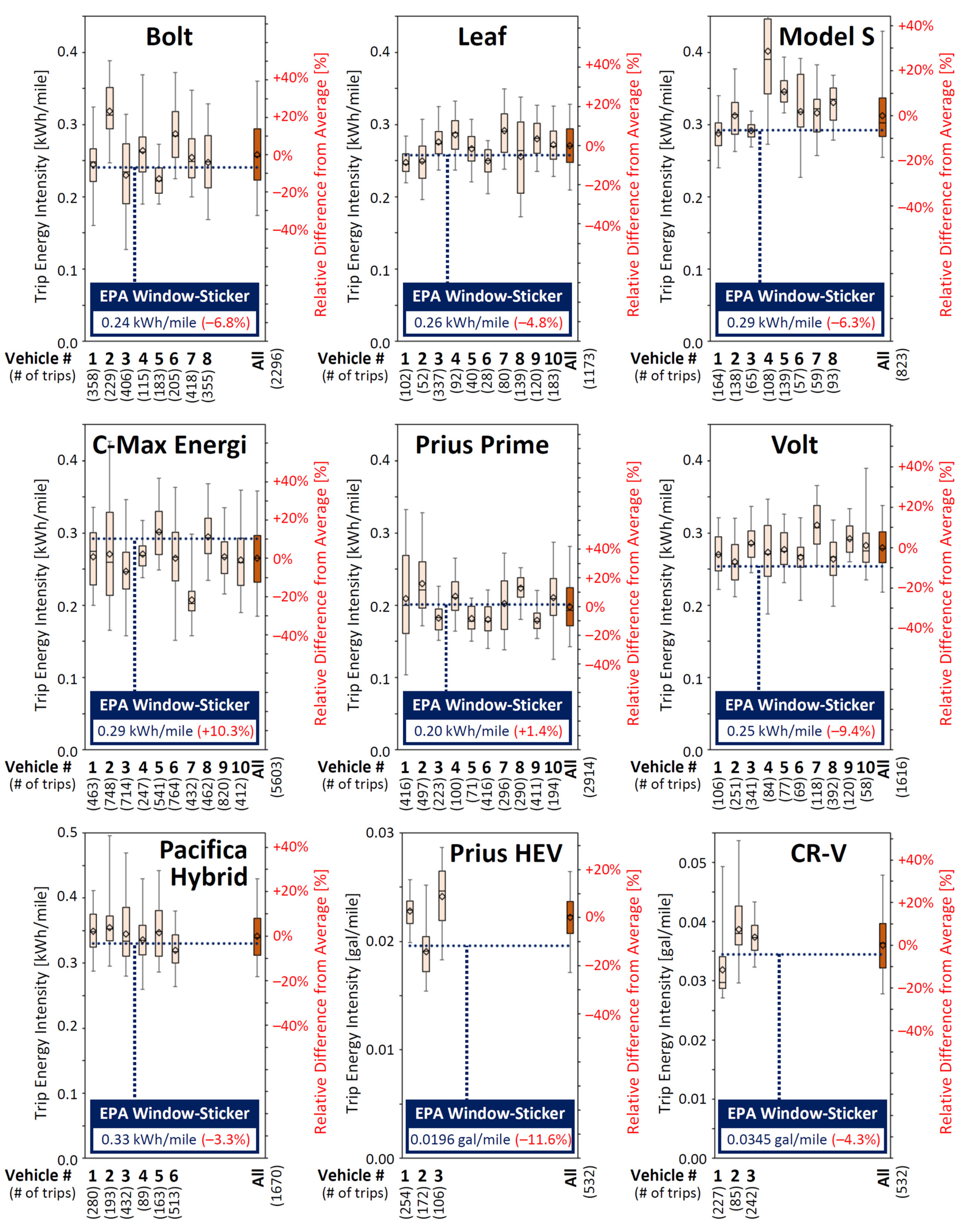
- For the vast majority of the considered individual vehicle owners, some of their trips have higher energy intensity than the window-sticker value, while some other trips have lower energy intensity (other than a few cases such as the Bolt owner #2 and Model S owner #5, the dashed line in Figure 1 lies between the 5th and 95th percentiles marked by the extension lines of box-plots);
- Window-sticker values can be reasonably good (within approximately ±10%) at predicting the average energy intensity across multiple vehicle owners (comparing the average value for darker tone box plots with the dashed line in Figure 1), but the average energy intensity for some individual vehicle owners can be off from the window-sticker value by more than 20%, such as the Model S owner #4 in Figure 1;
- Individual trips by vehicle owners may occasionally be different than the average across owners (reading the 5th and/or 95th extension lines on the secondary vertical axis in Figure 2) by more than 50%. By extent, the window-sticker values can also be off by more than 50% for some individual trips.
3. Model Calibration
- αT is a scaling factor that adjusts the total traction power at every time instant (calculated by FASTSim to account for acceleration, wind drag, rotational inertia, road slope, and tire rolling resistance).
- αM is a correction mass (in (kg)) to account for differences across vehicle owners in passenger and cargo weight from the default (136 kg) value in FASTSim.
- αA is a constant additional power (in (kW)) that takes the form of a correction term for auxiliary power, but is intended to also account for other unknown effects.
4. Results and Discussion
- Window-sticker-based prediction, in which the prediction for every trip is simply the combined cycle rating from the fuel economy guide [7].
- Baseline FASTSim models, as published by NREL in the 2018 public version of FASTSim [3]. It should be noted, however, that the public version of FASTSim does not include all vehicle models considered in the current study (Table 1). Thus, a “baseline” FASTSim model could not be examined for Pacfica Hybrid, Prius HEV, or CR-V.
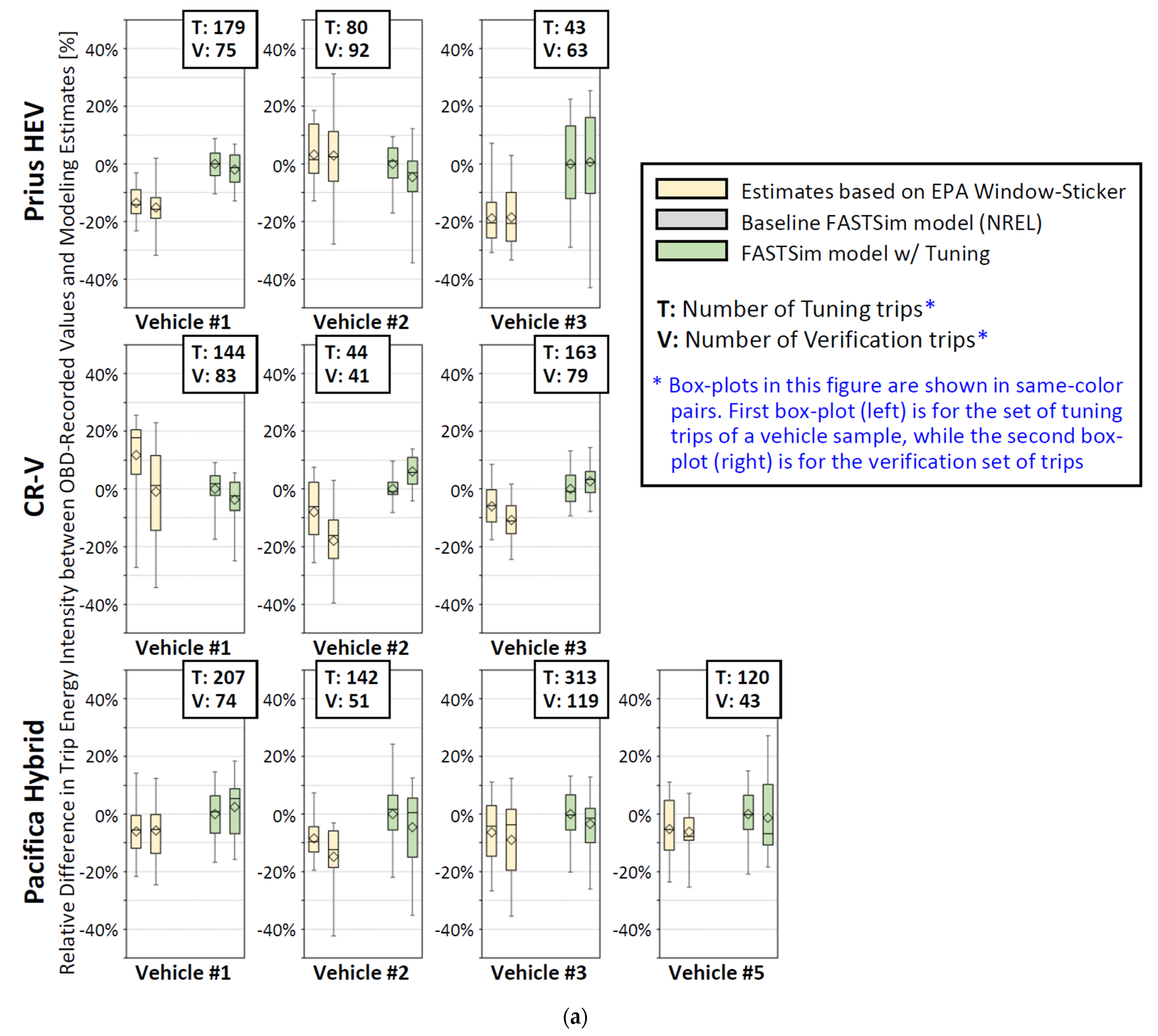
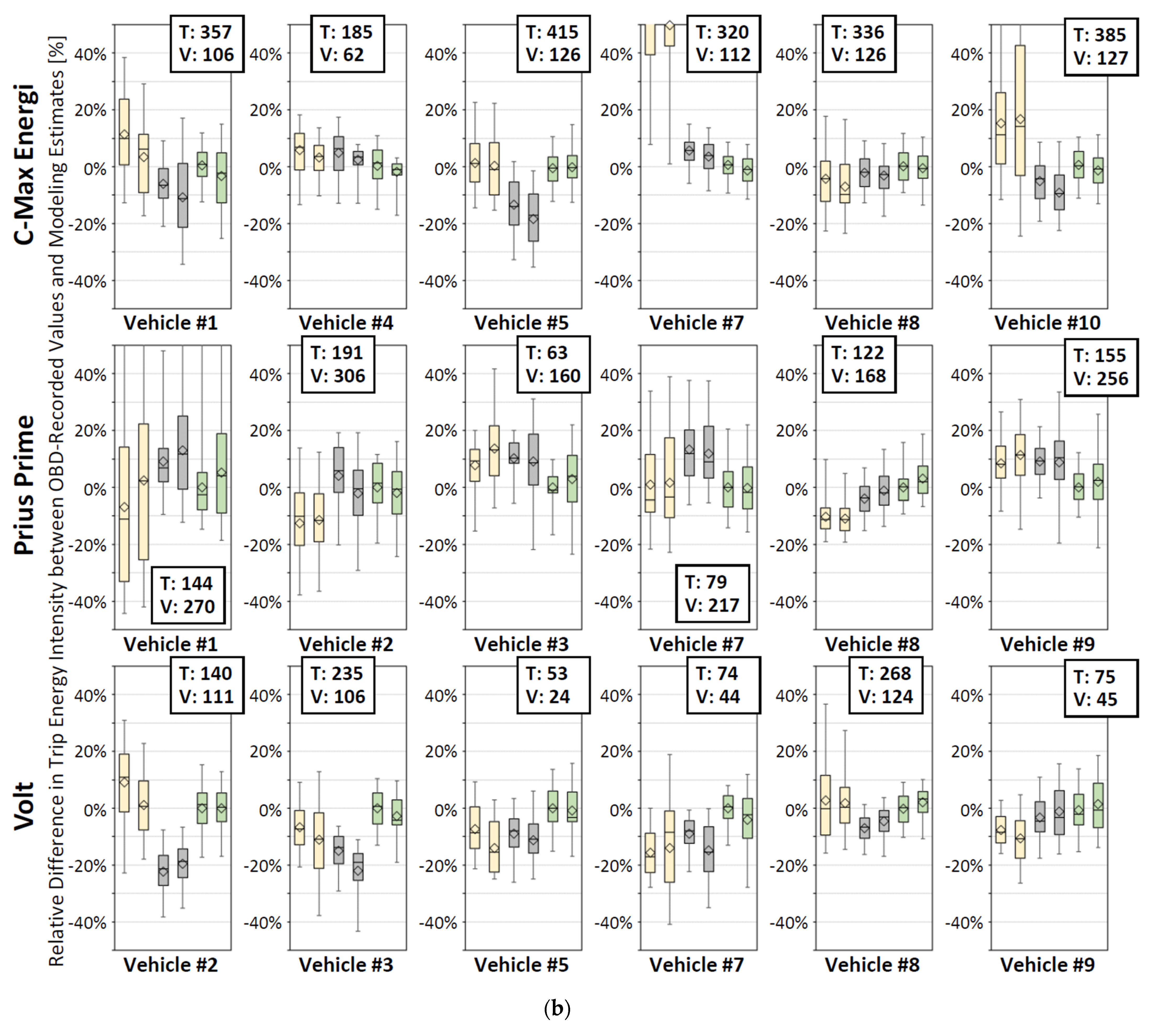
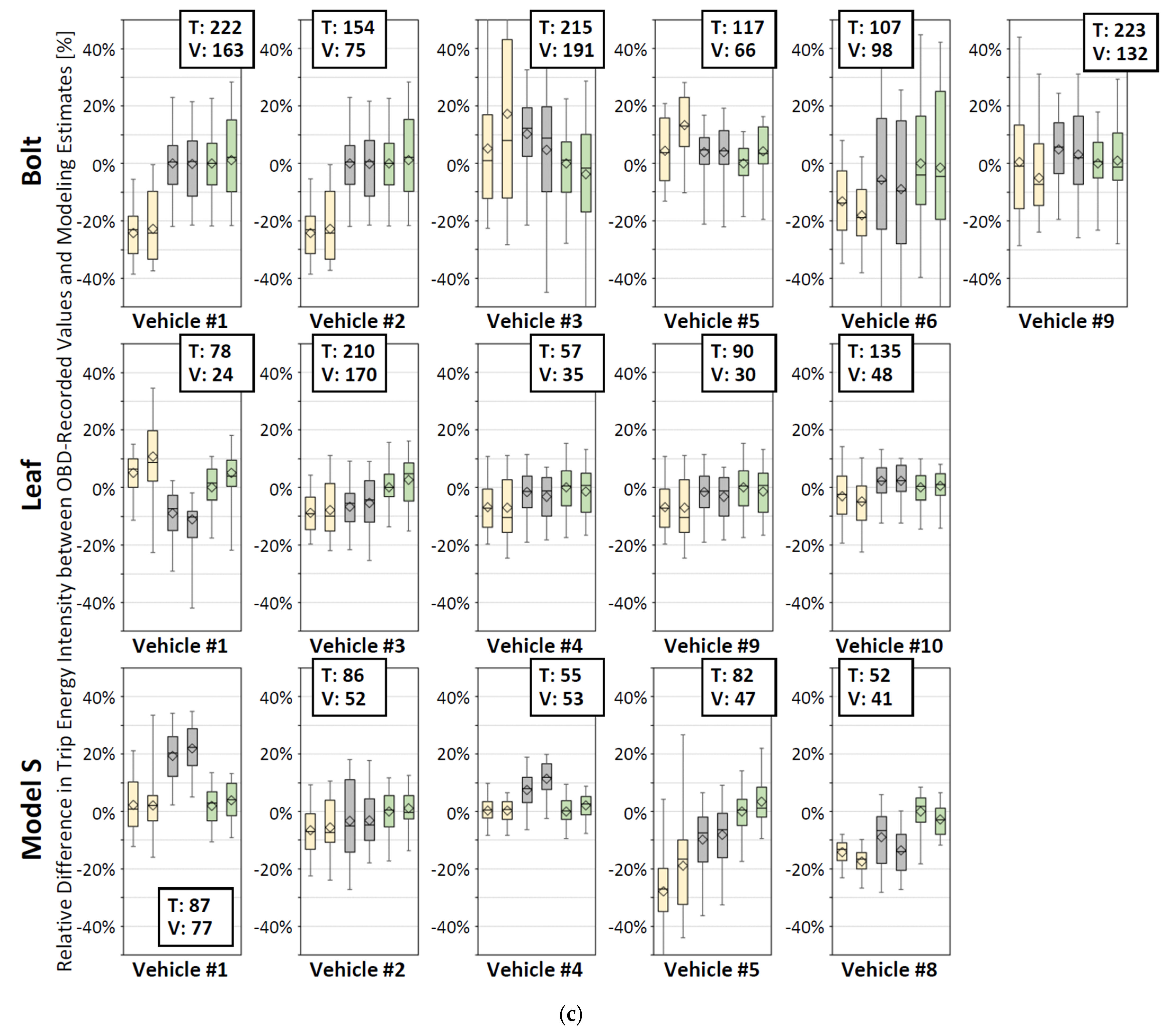
- FASTSim models with tuning, per the adopted calibration approach.
- The average value (diamond marker) for tuned FASTSim models for the tuning set of trips (left box-plot in the green color tone pairs) remains within ±1% for all vehicle samples of all considered vehicle models. This is an indication of success for the optimization process being able to find a good solution for the tuning parameter values, but not necessarily an indication that the tuned FASTSim models can generalize well.
- The average value for tuned FASTSim models for the verification set of trips (right box-plot in the green color tone pairs) is mostly within ±5%, with the exception of Bolt vehicle #1, CR-V vehicle #2, and Prius Prime vehicle #1, which have errors of −6.6%, +6.0%, and +5.2%, respectively.
- The average value for window-sticker based estimates (diamond marker in either of the yellow color tone box-plot pairs) is outside the bounds of ±10% on some vehicle samples across different vehicle models, with a few cases outside ±15% and one extreme case (C-Max Energi vehicle #7) exceeding 40%.
- The average value for baseline FASTSim (diamond marker in either of the gray color tone box-plot pairs) is mostly within ±15%, with the exception of Model S vehicle #1, Volt vehicles #2 and #3, C-Max Energi vehicle #5, which have errors of +22.0%, −22.3%, −22.0% and −19.4% respectively.
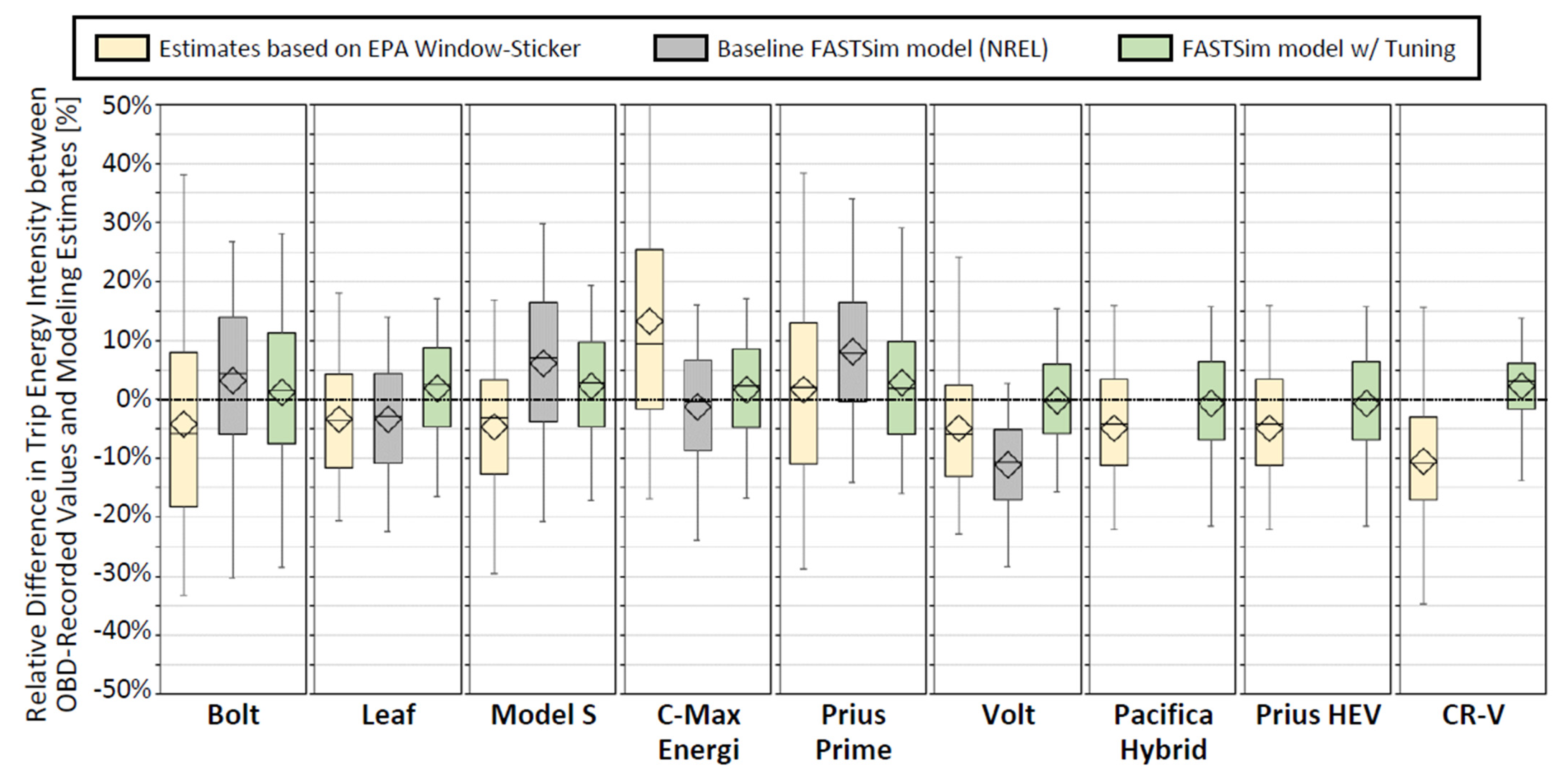
- The average value (diamond shape) for both window-sticker-based estimates (yellow color tone box plots in Figure 3) and baseline FASTSim (gray color tone box plots) remains mostly within ±10% error bounds, with the exception of C-Max Energi, and CR-V for window-sticker-based estimates, and Volt for baseline FASTSim.
- The average value for tuned FASTSim models (diamond shape of green color tone box plots in Figure 3) remains within ±3% error for all the studied vehicle models. The worst observed cases were for Prius Prime and CR-V, at +2.8% and +2.2%, respectively.
5. Conclusions
Author Contributions
Funding
Data Availability Statement
Acknowledgments
Conflicts of Interest
References
- Zhou, M.; Jin, H.; Wang, W. A Review of Vehicle Fuel Consumption Models to Evaluate Eco-Driving and Eco-Routing. Transp. Res. Part D 2016, 49, 203–218. [Google Scholar] [CrossRef]
- Argonne National Laboratory. Autonomie: Automotive System Design. Available online: https://www.autonomie.net/ (accessed on 18 October 2019).
- National Renewable Energy Laboratory. Future Automotive Systems Technology Simulator. Available online: http://www.nrel.gov/transportation/fastsim.html (accessed on 18 October 2019).
- US Department of Energy; Vehicle Technologies Office. Modeling and Simulation. Available online: https://energy.gov/eere/vehicles/vehicle-technologies-office-modeling-and-simulation (accessed on 18 October 2019).
- US Environmental Protection Agency. MOVES and Other Mobile Source Emissions Models. Available online: https://www.epa.gov/moves (accessed on 18 October 2019).
- California Air Resources Board. MSEI—Modeling Tools. Available online: https://ww2.arb.ca.gov/our-work/programs/mobile-source-emissions-inventory/msei-modeling-tools (accessed on 18 October 2019).
- US Department of Energy; Environmental Protection Agency. The Official U.S. Government Source for Fuel Economy Information. Available online: https://www.fueleconomy.gov/ (accessed on 18 October 2019).
- Islam, E.; Moawad, A.; Kim, N.; Rousseau, A. Vehicle Electrification Impacts on Energy Consumption for Different Connected-Autonomous Vehicle Scenario Runs. World Electr. Veh. J. 2020, 11, 9. [Google Scholar] [CrossRef] [Green Version]
- Kim, H.; Pyeon, H.; Park, J.; Hwang, J.; Lim, S. Autonomous Vehicle Fuel Economy Optimization with Deep Reinforcement Learning. Electronics 2020, 9, 1911. [Google Scholar] [CrossRef]
- Luo, Y.; Xiang, D.; Zhang, S.; Liang, W.; Sun, J.; Zhu, L. Evaluation on the Fuel Economy of Automated Vehicles with Data-Driven Simulation Method. Energy AI 2021, 3, 100051. [Google Scholar] [CrossRef]
- Hamza, K.; Chu, K.C.; Favetti, M.; Benoliel, P.; Karanam, V.; Laberteaux, K.; Tal, G. Validity Assessment and Calibration Approach for Simulation Models of Energy Efficiency of Light-Duty Vehicles; SAE World Congress: Detroit, MI, USA, 2020. [Google Scholar]
- UC-Davis ITS. eVMT Project. Available online: https://phev.ucdavis.edu/project/evmt-project/ (accessed on 18 October 2019).
- Jin, R.; Chen, W.; Simpson, T.W. Comparative studies of metamodelling techniques under multiple modelling criteria. Struct. Multidiscip. Optim. 2001, 23, 1–13. [Google Scholar] [CrossRef]
- Brooker, A.; Gonder, J.; Wang, L.; Wood, E.; Lopp, S.; Ramroth, L. FASTSim: A Model to Estimate Vehicle Efficiency, Cost and Performance; SAE World Congress: Detroit, MI, USA, 2015. [Google Scholar]


| Tuning Parameter Values | ||||
|---|---|---|---|---|
| Vehicle Model | Vehicle Sample ID | αT | αM [kg] | αA [kW] |
| Bolt | 1 | 0.94 | 173.9 | 0.071 |
| 2 | 0.94 | −14.2 | 2.084 | |
| 3 | 0.94 | −50.0 | 0.009 | |
| 5 | 0.94 | 60.3 | 0.689 | |
| 6 | 0.94 | 205.8 | 1.108 | |
| 9 | 0.94 | 29.3 | 0.823 | |
| (Group) | 0.94 | 36.9 | 0.899 | |
| Leaf | 1 | 0.98 | 243.2 | 0.839 |
| 3 | 0.98 | 217.5 | 0.878 | |
| 4 | 0.98 | 238.8 | 0.832 | |
| 9 | 0.98 | −5.5 | 0.741 | |
| 10 | 0.98 | −8.1 | 0.382 | |
| (Group) | 0.98 | 144.3 | 0.746 | |
| Model S | 1 | 0.96 | −50.0 | 0.000 |
| 2 | 0.96 | 224.1 | 0.782 | |
| 4 | 0.96 | 198.6 | 0.308 | |
| 5 | 0.96 | 167.6 | 2.765 | |
| 8 | 0.96 | 248.6 | 1.803 | |
| (Group) | 0.96 | 117.4 | 0.947 | |
| C-Max Energi | 1 | 0.92 | 154.9 | 0.655 |
| 4 | 0.92 | 105.7 | 0.000 | |
| 5 | 0.92 | 155.5 | 1.247 | |
| 7 | 0.92 | −50.0 | 0.000 | |
| 8 | 0.92 | 181.5 | 1.008 | |
| 10 | 0.92 | 194.5 | 0.310 | |
| (Group) | 0.92 | 118.0 | 0.486 | |
| Prius Prime | 1 | 0.96 | −18.1 | 0.545 |
| 2 | 0.96 | 26.1 | 0.933 | |
| 3 | 0.96 | 69.1 | 0.053 | |
| 7 | 0.96 | −27.6 | 0.000 | |
| 8 | 0.96 | 106.6 | 1.177 | |
| 9 | 0.96 | 82.4 | 0.150 | |
| (Group) | 0.96 | 54.7 | 0.445 | |
| Volt | 2 | 1.02 | 155.7 | 1.024 |
| 3 | 1.02 | 122.8 | 1.567 | |
| 5 | 1.02 | 226.8 | 0.670 | |
| 7 | 1.02 | 257.8 | 0.605 | |
| 8 | 1.02 | 73.2 | 0.364 | |
| 9 | 1.02 | 58.7 | 0.000 | |
| (Group) | 1.02 | 131.6 | 0.830 | |
| Pacifica Hybrid | 1 | 1.00 | 218.4 | 0.216 |
| 2 | 1.00 | 104.9 | 0.001 | |
| 3 | 1.00 | 221.3 | 0.954 | |
| 5 | 1.00 | 316.3 | 1.359 | |
| (Group) | 1.00 | 209.3 | 0.605 | |
| Prius HEV | 1 | 1.02 | −47.3 | 0.993 |
| 2 | 1.02 | −41.2 | 0.479 | |
| 3 | 1.02 | −10.7 | 0.559 | |
| (Group) | 1.02 | −44.9 | 0.889 | |
| CR-V | 1 | 1.02 | 57.6 | 0.212 |
| 2 | 1.02 | 159.1 | 2.295 | |
| 3 | 1.02 | 40.3 | 2.020 | |
| (Group) | 1.02 | 71.7 | 1.445 | |
Publisher’s Note: MDPI stays neutral with regard to jurisdictional claims in published maps and institutional affiliations. |
© 2021 by the authors. Licensee MDPI, Basel, Switzerland. This article is an open access article distributed under the terms and conditions of the Creative Commons Attribution (CC BY) license (https://creativecommons.org/licenses/by/4.0/).
Share and Cite
Hamza, K.; Chu, K.-C.; Favetti, M.; Benoliel, P.K.; Karanam, V.; Laberteaux, K.P.; Tal, G. Comparisons of Real-World Vehicle Energy Efficiency with Dynamometer-Based Ratings and Simulation Models. World Electr. Veh. J. 2021, 12, 161. https://doi.org/10.3390/wevj12040161
Hamza K, Chu K-C, Favetti M, Benoliel PK, Karanam V, Laberteaux KP, Tal G. Comparisons of Real-World Vehicle Energy Efficiency with Dynamometer-Based Ratings and Simulation Models. World Electric Vehicle Journal. 2021; 12(4):161. https://doi.org/10.3390/wevj12040161
Chicago/Turabian StyleHamza, Karim, Kang-Ching Chu, Matthew Favetti, Peter Keene Benoliel, Vaishnavi Karanam, Kenneth P. Laberteaux, and Gil Tal. 2021. "Comparisons of Real-World Vehicle Energy Efficiency with Dynamometer-Based Ratings and Simulation Models" World Electric Vehicle Journal 12, no. 4: 161. https://doi.org/10.3390/wevj12040161
APA StyleHamza, K., Chu, K.-C., Favetti, M., Benoliel, P. K., Karanam, V., Laberteaux, K. P., & Tal, G. (2021). Comparisons of Real-World Vehicle Energy Efficiency with Dynamometer-Based Ratings and Simulation Models. World Electric Vehicle Journal, 12(4), 161. https://doi.org/10.3390/wevj12040161